Optimal integration of different types of DGs in radial distribution system by using Harris hawk optimization algorithm

Abstract

The probable availability of renewable power sources is unexceptionable, and the government of India is setting high goals for the use of renewable energy. Renewable distributed generation (DG) reduces the need for fossil fuels, relieve environment change, and decrease radiations of CO₂ and other perfluorocarbons. DGs and capacitors are more desirable choices to balance power demand closer to the load centres than centralized power generation. Optimal position and capacity of DGs play an essential role in enhancing the performance of distribution systems in terms of system loss mitigation, voltage profile enhancement and stability concerns. This paper introduces Harris Hawk Optimization (HHO) and Teaching Learning-Based Optimization (TLBO) approaches for efficient distribution of different types of DGs in the radial distribution system (RDS) to enhance system loss minimization, voltage profile, yearly energy savings and decreasing the greenhouse gas emissions. The aim is to depreciate system energy losses, cost of energy losses and more reliable voltage regulation within the frame-work of RDS planning. Four different cases are considered to assess the suggested algorithms. Simulations are carried out on IEEE 33-bus and 69-bus test RDSs. The preponderance of the recommended approaches has been shown by analysing the results with techniques available in the literature. The comparison is made based on the power losses and voltage profile of RDS. The outcomes reveal that a significant decrease in power loss, enrichment of the voltage profile across the network and exactness of the suggested methods.

Keywords:

• Distributed Generation (DG)
• fossil fuels
• voltage profile
• power loss
• Harris Hawk Optimization (HHO)
• Teaching Learning-Based Optimization (TLBO)

PUBLIC INTEREST STATEMENT

Over the years, there have been many traditional and mathematical techniques studied to solve the Optimal allocation of Distributed Generation problem in Radial Distribution Systems. This problem can be considered as a nonlinear and nonconvex optimization problem with many local minima. The drawbacks of conventional optimization techniques like linear programming and gradient-based methods are that they are unable to handle non-linear and discrete functions and constraints are trapped at non-optimal local points. This article proposes Harris Hawk Optimization (HHO) and Teaching Learning-Based Optimization (TLBO) approaches for efficient allocation of different types of DGs in the radial distribution system (RDS) to reduce the total power losses, yearly energy costs, greenhouse gas emissions and enhance the voltage profile. The effectiveness of the proposed methodology is compared to the other well-known optimization methods that exist in literature and concluded that the proposed techniques are better in performance and yielding more optimal results.

1. Introduction

Today, centralized power generation is insufficient to satisfy the global energy demand. Around 13% of the world does not have access to electricity (https://ourworldindata.org/energy-access). In this context, DG has proven to be a viable alternative where electricity is produced close to the load centers. The renewable DG sources can be deliberately placed in radial distribution networks for providing environmental-friendly generation of electric power and improvement of overall performance of radial distribution networks. Even though DGs have many financial and environmental benefits, they impose some operational problems in RDS. These may include voltage rise, power quality, relay co-ordination problems caused by reverse power flow and voltage stability issues, etc. (Loong et al., 2011). Proper planning of DGs plays an essential role in enhancing the performance of distribution systems in terms of system loss mitigation, voltage profile enhancement and stability concerns. Hence, optimal DG allocation problem has been a global challenge for power system engineers.

Several researchers have used various optimization techniques to find the optimal size and its optimal locations, presenting a wide range of techniques from analytical to intelligent and Metaheuristic methods. Among the three, heuristic techniques have recently been commonly used to solve the optimal DG location and sizing problem. Mohsen et al. (2017) proposed Grey Wolf Optimization algorithm to find the optimal locations and sizes of photovoltaic (PV) and Wind Turbine (WT) based DGs in RDNs to minimize the losses. Imran Ahmad Quadri and Bhowmick (2018) introduced a CTLBO strategy, which manages both single and multi-objective function for optimum allocation of DGs in radial distribution systems to boost network loss reduction, voltage profile and annual energy savings. The optimum number of DGs is also being studied. The usefulness of this method is validated IEEE 33, 69 and 118 bus RDS. Kayalvizhi and Vinod Kumar (2018) proposed a new hybrid Grid-based Multi-objective Harmony Search algorithm for optimal planning and operation of DG in a distribution network. The DGs location, size and PF of diesel generators are optimized using the proposed algorithm to minimize energy loss, voltage deviation, and cost of DG. The effectiveness of the proposed algorithm is verified with IEEE 33, 69 and 85 bus RDS. Pazouki et al. (2016) use genetic algorithm of Matlab and Cplex solver of GAMS for optimal placement and sizing of combined heat and power (CHP) in RDS to minimize the cost, losses, reliability and voltage penalty. Paterakis et al. (2016) formulated RDS reconfiguration problem as multiobjective mathematical programming (MMP) problem with linear objective functions and constraints using mixed-integer linear programming (MILP) approach. The objectives considered were the minimization of the active power losses and reliability. Khosravi et al. (2018) use the bifurcation theory for investigation of the dynamic stability in a grid-connected wind turbine system based on Double Feed Induction Generator (DFIG). Mehdi Hosseini (2018) introduces a controller based on UPQC, which is able to compensate voltage sag directly and using ATP-EMTP software. Mokryani and Siano (2013) propose a hybrid optimization method for optimal allocation of wind turbines (WTs) that combines genetic algorithm (GA) and market-based optimal power flow (OPF). The GA is used to choose the optimal size while the market-based OPF to determine the optimal number of WTs at each candidate bus. The effectiveness of the method is demonstrated with an 84-bus RDS. Eroshenko et al. (2013) addresses the problem of DG siting and sizing optimization with subsequent equipment configuration assessment based on the combination of genetic algorithms and indicative analysis. Indicative analysis gives an opportunity to assess power system interaction with incident infrastructures and to take into account ecological, regulatory and other criteria, which makes the decision process more comprehensive and flexible. Genetic algorithm optimization is used to calculate initial data for final solution determination, which is very important for time-saving reasons. Sheng et al. (2015) propose improved nondominated sorting genetic algorithm–II (INSGA-II) for optimal planning of multiple DG units to minimize the losses, voltage deviation and maximize the voltage stability. The feasibility and effectiveness of the proposed algorithm have been tested on IEEE 33 bus RDS. Singh and Goswami (2009) propose a genetic algorithm-based method to determine the optimal location and size of the DGs in RDS to minimize the power loss.

Improvements in soft computing procedures have begun to advance several optimization algorithms for efficient integration of DGs in the radial distribution systems. Extensive research with the use of GA to efficiently distribute DGs in distribution networks described in (Carpinelli et al., 2001). Particle swarm optimization (Sheen et al., 2013) is another innovative technique popularly used in the distribution network for DG positioning. Adaptive particle swarm optimization (APSO) (Malekpour et al., 2013) is used to optimize the wind power generators and fuel cells to minimize electrical energy losses, cost of energy generated, total emissions produced and bus voltage deviation. Artificial Bee Colony (Nasiraghdam & Jadid, 2012) was used to optimize DG positioning to reduce investment costs. In addition to GA, ABC and PSO, researchers have developed several nature-inspired techniques like the honey bee mating algorithm (Niknam et al., 2011), cuckoo search algorithm (Moravej & Akhlaghi, 2013), bacterial foraging optimization (Mohamed Imran & Kowsalya, 2014), Firefly algorithm (Sulaiman et al., 2012), and Gravitational Search algorithm (Niknam et al., 2013) for efficient allocation of DGs and these techniques require proper tuning of parameters to prevent a non-optimal solution.

The main contributions of this work are summarized as follows:

The backward/forward sweep load flow algorithm was used to find the losses and bus voltages.

Applying the proposed HHO and TLBO algorithms to determine the optimal allocation of DG units in the radial distribution system to minimize the total losses.

The effectiveness of the proposed methodology is compared to the other well-known optimization methods using standard IEEE 33-bus and 69-bus distribution systems with different operating scenarios.

This paper is organized as follows: Section II presents the problem formulation including the main objective functions. Section III presents an overview of the HHO. Section IV presents the application of the HHO in DG allocation. Section V presents an overview of the TLBO. Section VI presents the application of the TLBO in DG allocation. In Section VII, the numerical results based on the test systems are presented. Finally, the conclusions and future directions are presented in Section VIII.

2. Problem formulation

2.1. Objective function

The objective function equality and inequality limitations are acquainted with optimal placing and sizing of DGs as follows:

(1) $f\left(\mathrm{x}\right)=\mathrm{m}\mathrm{i}\mathrm{n}\sum _{\mathrm{i}=1}^{\mathrm{b}}{\mathrm{R}}_{\mathrm{i}}{\ast \mathrm{I}}_{\mathrm{i}}^2$(1)

2.2. Constraints

Equality Constraints: The constraints for power balance requirements

(2) $P_{supply}+\sum _{k=1}^{NG}P{G}_k-P_L=P_d$(2)

(3) $Q_{supply}+\sum _{\mathrm{k}=1}^{NG}Q{G}_k-Q_L=Q_d$(3)

Inequality Constraints:

Generator constraints: The acceptable limitation of distribution systems should not extend to the highest possible allowable power generated from DGs, i.e.,

(4) $P{G}_k^{min}\le P{G}_k\le P{G}_k^{max}$(4)

(5) $Q{G}_k^{min}\le Q{G}_k\le Q{G}_k^{max}$(5)

(6) $0.95\le V{G}_k\le 1.05,\mathrm{k}=1,2,3\dots \dots .,nbus$(6)

Transformer constraints: The transformer‘s tap settings should be confined within the lowest and highest limits, i.e.

(7) $T_k^{min}\le T_k\le T_k^{max},\mathrm{k}=1,2,3\dots \dots .,nbus$(7)

Security constraints: Voltage at every load bus should be within its minimum and maximum operational bounds. Loadings over each line should not exceed its maximum loading limit, i.e.

(8) $V{L}_k^{min}\le V{L}_k\le V{L}_k^{max}$(8)

(9) $S{L}_k\le S{L}_k^{max},\mathrm{k}=1,2,3\dots \dots .,nbus$(9)

2.3. Economical analysis with DG integration

The mathematical models represented for evaluating the cost of energy losses, and cost component of DG power are given as follows.

2.3.1. Cost of energy losses (CEL)

The cost of energy loss is given by (Murthy & Kumar, 2013)

(10) $CEL=\left(APL\right)\ast \left(K_{pl}+K_{el}\ast L{s}_f\ast 8760\right)\mathrm{\$}$(10)

Ls_f is the loss factor and can be expressed as

(11) $L{s}_f=k\ast L_f+\left(1-k\right)\ast L_f^2$(11)

The values used in the estimation of the loss factor are: k = 0.2, Lf = 0.47, K_pl = 57.6923 $/kW, K_el = 0.00961538 $/kWh.

2.3.2. Cost component of DG for real and reactive power

Active power costs provided by DG can be determined by

(12) $\mathrm{C}\mathrm{o}\mathrm{s}\mathrm{t}\left(P_{dg}\right)=\mathrm{x}\ast P_{dg}^2+\mathrm{y}\ast P_{dg}+\mathrm{z}\mathrm{\$}/\mathrm{M}\mathrm{W}\mathrm{h}$(12)

Reactive power costs provided by DG can be determined by

(13) $Cost\left(Q_{dg}\right)=cost\left(S_{gmax}\right)-cost(\sqrt{S_{gmax}^2-Q_{dg}^2)}\ast m$(13)

(14) $S_{gmax}=\frac{1.1\ast P_{dg}}{cos\text{o}}$(14)

Where, x = 0, y = 20 and z = 0.25 are taken from (Murthy & Kumar, 2013). Cosϕ is the power factor of the DG. S_gmax = 0 for type-II DG. The value of m is in the range from 0.05 to 1. In this paper, the value of m is taken as 1.

3. Harris hawk optimization algorithm

Heidari and his collaborators suggested Harris hawk optimization (HHO) in 2019 (Heidari et al., 2019). The Harris hawk is a prey bird that exists as steady communities found in the southern side of Arizona, United States. Harris hawk’s main tactic to catch prey is “surprise pounce”, and it can also be recognized as the strategy of “seven kills”. In this winning strategy, many hawks try to strike together from different directions and at the same time concentrate on a perceived rabbit that falls outside the shield. The assault can be easily accomplished by catching the surprised victim in a couple of seconds, although sometimes, with regards to the prey’s escape capability and habits, the “seven kills” can include several, short length, and rapid dives near the victim for several minutes.

Harris hawks can display a diverse range of hunting styles depending on complex nature and prey’s escape patterns. When the best hawk (leader) bows down at the prey and gets lost, a switching tactic occurs, and one of the party members can continue the chase. In different circumstances, such switching activities could be examined as they are helpful for annoying the escaping rabbit. The main benefit of such collaborative tactics is that the Harris hawks can pursue to exhaustion the detected rabbit, which increases its weakness. It cannot restore its defensive capabilities by confusing the escaping prey. Finally, it cannot survive the challenged group besiege since one of the hawks, which is often the most effective and skilled, catches the exhausted rabbit quickly and exchanges it with other members.

Figure 1. Different stages of HHO (Heidari et al., 2019).

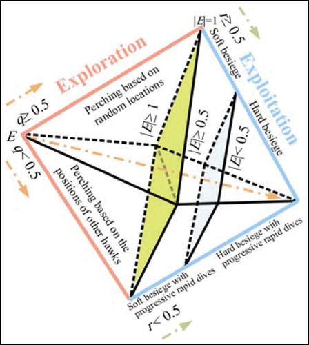
Generally, HHO is modelled into exploration and exploitation stages inspired by Harris hawks exploration of a prey, surprise pounce, and various attacking strategies. Different stages of HHO are shown in Figure 1. The major advantages of the HHO are its simplicity and have a few exploratory and exploitative mechanisms.

3.1. Exploration phase

The position of the hawk is changed in the exploration phase by random location and many other hawks and is given by equation (15)(15) $L\left(t+1\right)=\left\{\begin{array}{c}{L}_k\left(t\right)-d_1\left|L_k\left(t\right)-2d_{2}L\left(t\right)\right|\hspace{0.17em}r\ge 0.5\\ \left(L_r\left(t\right)-L_m\left(t\right)\right)-d_3\left(lb+d_4\left(u_{lim}-l_{lim}\right)\right)\\ r<0.5\end{array}\right.$(15) (Heidari et al., 2019)

(15) $L\left(t+1\right)=\left\{\begin{array}{c}{L}_k\left(t\right)-d_1\left|L_k\left(t\right)-2d_{2}L\left(t\right)\right|\hspace{0.17em}r\ge 0.5\\ \left(L_r\left(t\right)-L_m\left(t\right)\right)-d_3\left(lb+d_4\left(u_{lim}-l_{lim}\right)\right)\\ r<0.5\end{array}\right.$(15)

Where L is the hawk’s position, L_k is the position of chosen hawk randomly, L_r is the location of prey, t is the present iteration, u_lim and l_lim are the threshold limits of search area, d₁, d₂, d₃, d₄, and r are the five discrete random numbers in [0, 1]. The L_m is the average location of the present hawk’s community, and it can be calculated by using Equation (16)(16) $L_m\left(t\right)=\frac{1}{H}\sum _{p=1}^H{L}_p\left(t\right)$(16) .

(16) $L_m\left(t\right)=\frac{1}{H}\sum _{p=1}^H{L}_p\left(t\right)$(16)

Where L_p is the p^th hawk in the community, and H is the no. of hawks.

3.2. Transition from exploration to exploitation

The HHO algorithm can be translated from exploration to exploitation, and then the behaviour of the exploration is modified depending on the prey’s escaping strength. Mathematically, prey’s strength to escape can be measured as

(17) $S=2S_0(1-\frac{t}{T})$(17)

(18) $S_0=2d-1$(18)

Where T is the max no of iterations, S₀ is the initial strength produced arbitrary in [−1, 1], and d is a random number in [0, 1]. When the prey’s escaping strength “S” is greater than 1, HHO granted the hawks to hunt on various regions globally. On the other hand, HHO appeared to boost the local search of the best alternatives around the neighbourhood when the prey’s escaping strength is less than 1.

3.3. Exploitation phase

During this phase, the position of the hawk is changed according to the following scenarios. This behaviour is controlled based on the prey’s escape strength (S) and the chance for prey to escape successfully (q < 0.5) or not (Q > 0.5) before surprise bounce.

3.3.1. Soft besiege

This phase appears when q ≥ 0.5 and |S| ≥ 0.5 and by using Equation (19)(19) $D{M}_{s,k}=r_k\left(X_{s,kbest,k}-T_F{M}_{s,k}\right)$(19) , the hawk adjusts its position.

(19) $D{M}_{s,k}=r_k\left(X_{s,kbest,k}-T_F{M}_{s,k}\right)$(19)

Where S is the prey’s escaping strength, L_q is the position of prey, ΔL is the change in the prey position and present hawk position, and j is the dive strength. The j and ΔL are calculated by using Equations (20)(20) $X_{p,s,k}^{\hspace{0.17em}}=X_{p,s,k}^{\prime }+r_k\left(X_{q,s,k}^{\prime }-X_{p,s,k}^{\prime }\right)\mathrm{i}\mathrm{f}X{\prime }_{(total,p,k)}<X{\prime }_{(total,q,k)}$(20) and (21(21) $j=2\left(1-d_5\right)$(21) ) (Heidari et al., 2019)

(20) $X_{p,s,k}^{\hspace{0.17em}}=X_{p,s,k}^{\prime }+r_k\left(X_{q,s,k}^{\prime }-X_{p,s,k}^{\prime }\right)\mathrm{i}\mathrm{f}X{\prime }_{(total,p,k)}<X{\prime }_{(total,q,k)}$(20)

(21) $j=2\left(1-d_5\right)$(21)

Where d₅ is a random number in [0, 1] that modifies in each iteration.

3.3.2. Hard besiege

This phase appears when q ≥ 0.5 and |S| < 0.5. In this scenario, the hawk updates its position using Equation (22)(22) $L\left(\mathrm{t}+1\right)=L_q\left(t\right)-S\left|\mathrm{\Delta }\mathrm{L}\left(t\right)\right|$(22) (Heidari et al., 2019)

(22) $L\left(\mathrm{t}+1\right)=L_q\left(t\right)-S\left|\mathrm{\Delta }\mathrm{L}\left(t\right)\right|$(22)

3.3.3. Soft besiege with progressive rapid dives

This phase has happened when q < 0.5 and |S| ≥ 0.5. The hawk is slowly selecting the best possible dive for competitively capturing the prey. In this situation, the hawk’s new position is created as follows (Heidari et al., 2019)

(23) $\mathrm{Y}={\mathrm{L}}_{\mathrm{q}}\left(\mathrm{t}\right)-\mathrm{S}\left|\mathrm{j}{\mathrm{L}}_{\mathrm{q}}\left(\mathrm{t}\right)-\mathrm{L}\left(\mathrm{t}\right)\right|$(23)

(24) $\mathrm{Q}=\mathrm{Y}+\mathrm{a}\ast \mathrm{L}\mathrm{e}\mathrm{v}\mathrm{y}\left(\mathrm{N}\right)$(24)

Where Y and Q are two recently produced hawks, j is the leaping power, N is the no of dimensions, a is an N dimension random vector, and Levy is the levy flight function that can be computed as

(25) $Levy\left(m\right)=0.01\ast \frac{\mu \ast \sigma }{{\left|\vartheta \right|}^{1/\beta }}$(25)

Where μ, ϑ are two separate random numbers created from the normal distribution, and σ is described as

(26) $\sigma ={\left(\frac{\mathrm{\Gamma }\left(1+\gamma \right)\ast sin\left(\frac{\pi \gamma }{2}\right)}{\mathrm{\Gamma }\left(\frac{1+\gamma }{2}\right)\ast \gamma \ast 2^{\left(\frac{\gamma -1}{2}\right)}}\right)}^{\frac{1}{\beta }}$(26)

Where γ is a constant and set to 1.5, the location of the hawk is modified by using Equation (27)(27) $L\left(t+1\right)=\left\{\begin{array}{c}YIfF\left(Y\right)<F\left(L\left(t\right)\right)\\ QIfF\left(Q\right)<F\left(L\left(t\right)\right)\end{array}\right.$(27) in this phase.

(27) $L\left(t+1\right)=\left\{\begin{array}{c}YIfF\left(Y\right)<F\left(L\left(t\right)\right)\\ QIfF\left(Q\right)<F\left(L\left(t\right)\right)\end{array}\right.$(27)

Where F is the fitness function, Y and Q are two solutions derived from Equations (23)(23) $\mathrm{Y}={\mathrm{L}}_{\mathrm{q}}\left(\mathrm{t}\right)-\mathrm{S}\left|\mathrm{j}{\mathrm{L}}_{\mathrm{q}}\left(\mathrm{t}\right)-\mathrm{L}\left(\mathrm{t}\right)\right|$(23) and (24(24) $\mathrm{Q}=\mathrm{Y}+\mathrm{a}\ast \mathrm{L}\mathrm{e}\mathrm{v}\mathrm{y}\left(\mathrm{N}\right)$(24) ).

3.3.4. Hard besiege with progressive rapid dives

This is the last scenario and appears when q < 0.5 and |S| < 0.5. In this condition, the following two new solutions are created (Heidari et al., 2019)

(28) $\mathrm{Y}={\mathrm{L}}_{\mathrm{q}}\left(\mathrm{t}\right)-\mathrm{S}\left|\mathrm{j}{\mathrm{L}}_{\mathrm{q}}\left(\mathrm{t}\right)-{\mathrm{L}}_{\mathrm{m}}\left(\mathrm{t}\right)\right|$(28)

(29) $\mathrm{Q}=\mathrm{Y}+\mathrm{a}\ast \mathrm{L}\mathrm{e}\mathrm{v}\mathrm{y}\left(\mathrm{N}\right)$(29)

Where L_m is the average location of the hawks in the current community. The position of the hawk is subsequently modified as

(30) $\mathrm{L}\left(\mathrm{t}+1\right)=\left\{\begin{array}{c}YIfF\left(Y\right)<F\left(L\left(\mathrm{t}\right)\right)\\ QIfF\left(Q\right)<F\left(L\left(\mathrm{t}\right)\right)\end{array}\right.$(30)

4. Application of Harris hawk optimization (HHO) algorithm for solving the objective function

The parameters of the HHO algorithm taken for this study are: the number of hawks (population size) is set to 100, and the maximum number of iterations is 50. In the test system, the HHO algorithm is run 50 times with the different randomly generated initial solutions.

4.1. Algorithm

The sequential steps involved in solving the problem of optimal allocation of DGs using the HHO algorithm are given below.

Step 1) Define objective function subjected to equality and inequality constraints of the design variables and read the line and load data.

Step 2) Initialize the number of hawk searches within upper and lower limits of DGs sizes in kW, locations of DGs, HHO parameters and maximum Number of iterations T.

Step 3) Set iteration count k = 1.

Step 4) Using forward-backward load flow, determine objective function value using Equation (1)(1) $f\left(\mathrm{x}\right)=\mathrm{m}\mathrm{i}\mathrm{n}\sum _{\mathrm{i}=1}^{\mathrm{b}}{\mathrm{R}}_{\mathrm{i}}{\ast \mathrm{I}}_{\mathrm{i}}^2$(1) for each search hawk.

Step 5) Identify the best hawk (Lr), which has given the best objective function value.

Step 6) for each hawk Lp, Update the values of S, S0 and j by using Equations (17)(17) $S=2S_0(1-\frac{t}{T})$(17) , (18(18) $S_0=2d-1$(18) ) and (21(21) $j=2\left(1-d_5\right)$(21) ) respectively.

Step 7) Check if S ≥ 1, update the hawk’s position by using Equation (15)(15) $L\left(t+1\right)=\left\{\begin{array}{c}{L}_k\left(t\right)-d_1\left|L_k\left(t\right)-2d_{2}L\left(t\right)\right|\hspace{0.17em}r\ge 0.5\\ \left(L_r\left(t\right)-L_m\left(t\right)\right)-d_3\left(lb+d_4\left(u_{lim}-l_{lim}\right)\right)\\ r<0.5\end{array}\right.$(15) otherwise go to Step 8.

Step 8) Check if S ≥ 0.5, go to Step 9 otherwise go to Step 10.

Step 9) Check if q ≥ 0.5, update the hawk’s position by using Equation (19)(19) $D{M}_{s,k}=r_k\left(X_{s,kbest,k}-T_F{M}_{s,k}\right)$(19) otherwise update by using Equation (27)(27) $L\left(t+1\right)=\left\{\begin{array}{c}YIfF\left(Y\right)<F\left(L\left(t\right)\right)\\ QIfF\left(Q\right)<F\left(L\left(t\right)\right)\end{array}\right.$(27) and go to Step 11.

Step 10) Check if q ≥ 0.5, update the hawk’s position by using Equation (22)(22) $L\left(\mathrm{t}+1\right)=L_q\left(t\right)-S\left|\mathrm{\Delta }\mathrm{L}\left(t\right)\right|$(22) otherwise update by using Equation (30)(30) $\mathrm{L}\left(\mathrm{t}+1\right)=\left\{\begin{array}{c}YIfF\left(Y\right)<F\left(L\left(\mathrm{t}\right)\right)\\ QIfF\left(Q\right)<F\left(L\left(\mathrm{t}\right)\right)\end{array}\right.$(30) and go to Step 11.

Step 11) Increment the iteration count k by 1 and Check if (Number of iterations < maximum Number of iterations) then go to Step 4 otherwise go to Step 12.

Step 12) Return the final best solution stored (DG Sizes and locations).

Step 13) Run the load flow and determine the power losses and voltage profiles.

4.2. Flowchart

The flowchart of HHO algorithm for optimal placement and sizing of DGs is illustrated in Figure 2.

Figure 2. Flowchart of HHO algorithm.

5. Teaching Learning-Based Optimization (TLBO) algorithm

The Teaching-Learning-Based Optimization (TLBO) algorithm is introduced by Rao et al. (2011) in 2011 using the influence of a teacher on learners. As compared with similar type of nature-inspired algorithms, namely, artificial bee colony (ABC), differential evaluation (DE) and Particle Swarm Optimization (PSO). TLBO is characterized by less computational effort and high consistency in providing the global solution for continuous nonlinear optimization problems. Basically the TLBO simulates the traditional teaching-learning process in a classroom. In the assumptions, the learning may take place in two phases like (i) through teacher (known as teacher phase) and (ii) interaction with co-learners/classmates (known as learner phase). Similar to the population-based algorithms, in TLBO, the number of students or group of students considered as population, the number of subjects as design variables of the optimization problem, the best solution among all population is treated as teacher and results of the learners as the fitness function. In this section, the basic operations involved in teacher phase and learner phase are explained briefly.

5.1. Teacher phase

In this phase, the students learn from the teacher and teacher keeps an effort to increase the mean of results of the students by conveying knowledge among them. Let Sn (n = 1, 2, 3, …. l) is the number of learners (population) and Sm (m = 1, 2, 3, … s) is the number of subjects (design variables in the optimization problem). Consider the sequential teaching-learning process (iteration) and at any sequence k, the mean result of a subject “s” as M(s, k). In the entire learners, the best learner who secured best mean result in all the subjects is treated as teacher in that iteration and denoted as X_total-k_best,k. In general, the teacher puts his maximum effort to increase the knowledge level of all the students, but the rate of learning depends on the quality of the teacher as well as learners in that class. This fact is expressed in Equation (31)(31) $D{M}_{s,k}=r_k\left(X_{s,kbest,k}-T_F{M}_{s,k}\right)$(31) as the difference between the best learner and mean of the remaining class.

(31) $D{M}_{s,k}=r_k\left(X_{s,kbest,k}-T_F{M}_{s,k}\right)$(31)

where X_s,kbest,k is the result of best learner (or teacher) in the subject “s”, rk is uniformly distributed random number between [0, 1], T_F is the teaching quality factor, which is the root cause for improving or change the mean result of the entire class in that subject M_s,k. The value of T_F can be either 1 or 2 and it decided randomly with equal probability as defined in Equation (32)(32) $T_F=round\left[1+rand\left(0,1\right)\left\{2-1\right\}\right]$(32) .

(32) $T_F=round\left[1+rand\left(0,1\right)\left\{2-1\right\}\right]$(32)

Note here, T_F is not an input parameter and can be generated in the process of TLBO algorithm using Equation (32)(32) $T_F=round\left[1+rand\left(0,1\right)\left\{2-1\right\}\right]$(32) . Using difference mean defined in Equation (31)(31) $D{M}_{s,k}=r_k\left(X_{s,kbest,k}-T_F{M}_{s,k}\right)$(31) , the current solution is updated in teaching phase as given in Equation (33)(33) $X_{l,s,k}^{\prime }=X_{l,s,k}+D{M}_{s,k}$(33) .

(33) $X_{l,s,k}^{\prime }=X_{l,s,k}+D{M}_{s,k}$(33)

All the updated $X_{l,s,k}^{\prime }$ values are accepted and carry forward for the next cycle/iteration as input, if they produce better function value else, remain same.

5.2. Learner phase

This phase simulates the cooperative learning process in which student can also gain new knowledge by interacting with other classmates, particularly from those who have better knowledge than him/her. This phenomenon is modelled here with brief explanatory.

Let consider two students randomly Sp and Sq and their updated solutions at the end of teaching phase as$X_{total,p,k}^{\prime }\ne X_{total,q,k}^{\prime }$. By interacting both, their knowledge levels are updated as Equation (34) in the maximization problem.

(34a) $X_{p,s,k}^{\hspace{0.17em}}=X_{p,s,k}^{\prime }+r_k\left(X_{p,s,k}^{\prime }-X_{q,s,k}^{\prime }\right)\mathrm{i}\mathrm{f}X{\prime }_{(total,p,k)}>X{\prime }_{(total,q,k)}$(34a)

(34b) $X_{p,s,k}^{\hspace{0.17em}}=X_{p,s,k}^{\prime }+r_k\left(X_{q,s,k}^{\prime }-X_{p,s,k}^{\prime }\right)\mathrm{i}\mathrm{f}X{\prime }_{(total,p,k)}<X{\prime }_{(total,q,k)}$(34b)

Note here Equation (34) can be reversed for minimization problem and the accepted values can carry forward to the next cycle, if updated values produce the better solution, else remain the same.

6. Application of Teaching Learning-Based Optimization (TLBO) algorithm for solving the objective function

The parameters of the TLBO algorithm taken for this study are: the population size and the maximum iteration number are taken as 100 and 50, respectively.

6.1. Algorithm

Step 1) Define the objective function subjected to equal and inequal constraints of the design variables.

Step 2) Initialize the population size equal to number of learners and design variables equal to the sizes of DGs and locations.

Step 3) Using forward-backward load flow, determine objective function value using Equation (1)(1) $f\left(\mathrm{x}\right)=\mathrm{m}\mathrm{i}\mathrm{n}\sum _{\mathrm{i}=1}^{\mathrm{b}}{\mathrm{R}}_{\mathrm{i}}{\ast \mathrm{I}}_{\mathrm{i}}^2$(1) .

Step 4) Set iteration count k = 1 and identify the best population/learner which has given best objective function value and treat that learner as a teacher. Also, determine the mean of all the population.

Step 5) Update the existing solutions using Equations (31)(31) $D{M}_{s,k}=r_k\left(X_{s,kbest,k}-T_F{M}_{s,k}\right)$(31) –(33(33) $X_{l,s,k}^{\prime }=X_{l,s,k}+D{M}_{s,k}$(33) ) and carry forward all accepted solutions if they result in a better solution than the current teacher.

Step 6) Using Equation (34) modify the solutions obtained in step 5 and carry forward all accepted solutions if they result in a better solution than the current teacher.

Step 7) save the current best teacher and repeat steps 4 to 6 until iteration count reaches to its maximum.

Step 8) At the end, print the best solution/teacher as the optimal solution and plot the saved best teacher record of all iterations as convergence characteristics and stop.

6.2. Flowchart

The flowchart of TLBO algorithm for optimal placement and sizing of DGs is illustrated in Figure 3.

Figure 3. Flowchart of TLBO algorithm.

7. Results and discussions

This division summarizes simulation results of the 33-bus, 69-bus (Murthy & Kumar, 2013) IEEE test systems using the prescribed methods for DG integration. In this paper, DG locations are categorically studied with single DG, two DGs and three DGs of four Types of DGs (Kansal et al., 2013). HHO and TLBO algorithms are utilized to decide the optimal position and size of the DGs to reduce the power losses. The proposed technique can be implemented for any number of DGs, but for reliability, the number of DGs is limited to three. The proposed optimization algorithms have been evaluated using the MATLAB program, which is implemented in a PC having Intel Core i5-4210U processor, up to 1.7 GHz and 8GB of RAM memory. The simulation results exhibit the usefulness of the suggested techniques for voltage control and decreasing the losses by combining the several types of DGs. Parameters are taken from (Murthy & Kumar, 2013) to plan the cost of DG and Energy Losses. In this article, the following summaries are presented to address the effect of different types of DGs on the system.

Scenario-1: System performance without integrating the DG (Base case)

Scenario-2: System performance with Type-I DG integration.

Scenario-3: System performance with Type-II DG integration.

Scenario-4: System performance with Type-III DG integration.

Scenario-5: System performance with Type-IV DG integration.

Scenario-6: Economical Analysis with DG integration.

7.1. Scenario-1: System performance without integrating the DG

7.1.1. 33-bus system

The 33-bus system consists of 32 branches. The rated voltage is 12.66 kV. The cumulative real and reactive demand on the system is 3715 kW and 2300 kVAR respectively. The minimum voltage of 0.9037 p.u is observed at bus number 18, which is outside of the prescribed limit of ±5% after executing the distribution power flow algorithm by using the forward-backward method (Babu et al., 2018). Moreover, the cumulative active power loss of the system is 210.9876 kW, and the cumulative reactive loss of the system is 143.1284 kVAR. It is recognized that 5.68% of the power is absorbed in the form of active power loss in the system. The regulation of voltage in the system is 9.63%.

7.1.2. 69-bus system

The 69-bus system consists of 68 branches. The rated voltage is 12.66 kV. The cumulative real and reactive demand on the system is 3802.1 kW and 2694.6 kVAR respectively. The maximum voltage deviation occurred at bus 65th, and it is the worst among all other busses. The voltage at the 65th bus is 0.9092 p.u. Moreover, the cumulative active power loss of the system is 225 kW, and the cumulative reactive loss of the system is 102.1647 kVAR. It can be noticed that 5.92% of power is absorbed in the form of active power loss in the system. The regulation of voltage in the system is 9.08%.

Figure 4. Bus voltages with and without Type-I DGs deployment and the effect of the number of DGs on loss minimization for 33- and 69-bus systems.

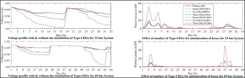
7.2. Scenario-2: System performance with Type-I DG integration

7.2.1. 33-bus system

Results of placing Type-I DGs by HHO and TLBO technique yields in the reduction of power loss, better voltage profile and improved savings which are shown in Table 1. The power losses reduced by 47.76%, 58.7% and 65.53% for single, two and three DGs placed respectively for HHO and 47.53%, 58.69% and 65.51% for TLBO. Also, the voltage profile enriched substantially with the placement of multiple DGs. The minimum voltage noticed was 0.9685, 0.9681 and 0.9426 p.u with three, two and single DG respectively for HHO and 0.9684, 0.9680 and 0.9426 p.u for TLBO.

Table 1. Comparison of simulation results of HHO and TLBO type-I DG units for 33-bus system

Method	Optimal Size of DG and Location			Total Size (kW)	Total Active Power Losses (kW)	Total Reactive Power Losses (kVAR)	% Active Power Loss Reduction	Vmin,p.u
Without DG	NA			NA	210.9876	143.1284	NA	0.9037
Single DG Unit
HHO	2584.1287 (6)			2584.1287	110.214	81.4524	47.76	0.9426
TLBO	2584.5546 (6)			2584.5546	110.706	81.4517	47.53	0.9426
GAMS (Murty & Kumar, 2019)	2589.52 (6)			2589.52	110.69	NA	47.53	0.9433
WOA (Prakash & Lakshminarayana, 2018)	2589.6(6)			2589.6	111	81.69	47.39	0.9424
HGWO (Sanjay et al., 2017)	2590(6)			2590	111.018	NA	47.38	0.9455
KHA (ChithraDevi et al., 2017)	2590.2126(6)			2590.2126	111.0188	81.7167	47.38	0.9424
SKHA (ChithraDevi et al., 2017)	2590.215(6)			2590.215	111.0188	81.7167	47.38	0.9424
Hybrid (Kansal et al., 2016)	2490(6)			2490	111.17	NA	47.31	NA
PSO (Kansal et al., 2016)	2590(6)			2590	111.03	NA	47.38	NA
HSA-PABC (Muthukumar & Jayalalitha, 2016)	2598(6)			2598	111.03	NA	47.38	0.9425
Dragonfly (Suresh & Belwin, 2018)	2590.2(6)			2590.2	111.033	81.6859	47.37	0.9424
2-DG Units
HHO	863.0261 (13)	1139.0726 (30)		2002.0987	87.1377	59.765	58.7	0.9681
TLBO	846.1427 (13)	1156.9739 (30)		2003.1166	87.1503	59.7918	58.69	0.968
GAMS (Murty & Kumar, 2019)	851.05(13)	1157.57 (30)		2008.62	86.87	NA	58.82	0.9684
HGWO (Sanjay et al., 2017)	852 (13)	1158 (30)		2010	87.164	NA	58.69	0.9714
KHA (ChithraDevi et al., 2017)	1241.714 (29)	824.4876 (13)		2066.2016	87.426	60.2091	58.56	0.9667
SKHA (Kansal et al., 2016)	851.6319(13)	1157.5892 (30)		2009.2211	87.1656	59.8129	58.69	0.9685
Hybrid (Kansal et al., 2016)	830(13)	1110 (30)		1940	87.28	NA	58.63	NA
PSO (Kansal et al., 2016)	850(13)	1160 (30)		2010	87.17	NA	58.68	NA
MINLP (Kaur et al., 2014)	850(13)	1150 (30)		2000	87.16	NA	58.69	NA
3-DG Units
HHO	811.7493(13)	1051.6753(24)	1045.9353(30)	2909.3599	72.718	50.6231	65.53	0.9685
TLBO	798.8176(13)	1090.2829(24)	1053.4248(30)	2942.5253	72.7702	50.6588	65.51	0.9684
GAMS (Murty & Kumar, 2019)	801.22(13)	1091.31(24)	1053.59(30)	2946.12	72.49	NA	65.64	0.9686
WOA (Prakash & Lakshminarayana, 2018)	856.678(13)	772.488(25)	1072.83(30)	2701.996	73.75	51.03	65.05	0.9688
HGWO (Sanjay et al., 2017)	802(13)	1090(24)	1054(30)	2,946	72.784	NA	65.5	0.9714
KHA (ChithraDevi et al., 2017)	914.9803(24)	750.1998(14)	1142.4045(30)	2807.5846	73.2968	51.016	65.26	0.9701
SKHA (ChithraDevi et al., 2017)	1053.6346(30)	1091.385(24)	801.8118(13)	2946.8314	72.7853	50.6814	65.50	0.9687
Hybrid (Kansal et al., 2016)	790(13)	1070(24)	1010(30)	2870	72.89	NA	65.45	NA
PSO (Kansal et al., 2016)	770(14)	1090(24)	1070(30)	2930	72.79	NA	65.5	NA
HSA-PABC (Muthukumar & Jayalalitha, 2016)	1369(6)	791(3)	820(28)	2980	99.79	NA	52.7	0.9398

7.2.2. 69-bus system

Table 2 illustrates the simulation results of placing Type-I DGs by HHO and TLBO techniques. The power losses are decreased by 63.02%, 68.14% and 69.14% for single, two and three DGs placed respectively for HHO and 63.01%, 68.14% and 69.14% for TLBO. The voltage regulation is also enhanced with multiple DGs placement. The minimum voltage detected was 0.9792, 0.9789 and 0.9683 p.u with 3 DGs, 2 DGs and 1 DG respectively for HHO and 0.9792, 0.9789 and 0.9683 p.u with 3 DGs, 2 DGs and 1 DGs respectively for TLBO. Figure 4 shows the bus voltages with and without type-I DGs deployment and the effect of the number of DGs on loss minimization for 33- and 69-bus systems. The convergence characteristic curves of the proposed HHO and TLBO algorithms for optimal placement and sizing of type-I DGs are shown in Figures 5 and 6 for 33- and 69-bus RDS respectively.

Table 2. Comparison of simulation results of HHO and TLBO type-I DG units for 69-bus system

Method	Optimal Size of DG			Total Size of DG(kW)	Total Active Power Losses (kW)	Total Reactive Power Losses (kVAR)	% Active Power Loss Reduction	Vmin,p.u
Without DG	NA			NA	225	102.1647	NA	0.9092
Single DG Unit
HHO	1872.7(61)			1872.7	83.204	40.536	63.02	0.9683
TLBO	1872.7(61)			1872.7	83.224	40.5361	63.01	0.9683
EHO (Prasad et al., 2019)	1873.6(61)			1873.6	83.23	40.54	63	0.9683
Dragonfly (Suresh & Belwin, 2018)	1872.7(61)			1872.7	83.22	40.57	63.01	0.9685
HGWO (Sanjay et al., 2017)	1872(61)			1872	83.222	NA	63.01	0.9682
KHA (ChithraDevi et al., 2017)	1864.6446(61)			1864.6446	81.6003	39.8185	62.99	0.9689
SKHA (ChithraDevi et al., 2017)	1864.6376(61)			1864.6376	81.6003	39.8185	62.99	0.9689
Hybrid (Kansal et al., 2016)	1810(61)			1810	83.37	NA	62.95	NA
PSO (Kansal et al., 2016)	1870(61)			1870	83.22	NA	63.01	NA
2-DG Units
HHO	532.1422(17)	1780.7918(61)		2312.934	71.6771	35.9419	68.14	0.9789
TLBO	531.8405(17)	1781.4909(61)		2313.3314	71.6771	35.9413	68.14	0.9789
HGWO (Sanjay et al., 2017)	531(17)	1781(61)		2312	71.674	NA	68.14	0.9799
KHA (ChithraDevi et al., 2017)	972.1609(51)	1726.9813(61)		2699.1422	77.0354	37.5038	65.76	0.973
SKHA (ChithraDevi et al., 2017)	522.9145(17)	1778.97(61)		2301.8845	70.4092	35.342	68.71	0.9792
Hybrid (Kansal et al., 2016)	520(17)	1720(61)		2240	71.8	NA	68.09	NA
PSO (Kansal et al., 2016)	1780(17)	530(61)		2310	71.68	NA	68.14	NA
3-DG Units
HHO	542.1997(11)	372.6548(17)	1715.8958(61)	2630.7503	69.431	34.9611	69.14	0.9792
TLBO	528.3797(11)	380.1178(17)	1725.5912(61)	2634.0887	69.4311	34.9607	69.14	0.9792
HGWO (Sanjay et al., 2017)	527(11)	380(17)	1718(61)	2625	69.425	NA	69.14	0.9799
KHA (ChithraDevi et al., 2017)	549.1027(15)	1768.4752(61)	1013.9691(49)	3331.547	69.1977	31.9783	69.25	0.9792
SKHA (ChithraDevi et al., 2017)	370.8802(11)	527.1736(17)	1719.0677(61)	2617.1215	68.1523	34.3566	69.71	0.9792
Hybrid (Kansal et al., 2016)	510(11)	380(17)	1670(61)	2560	69.54	NA	69.09	NA
PSO (Kansal et al., 2016)	460(11)	440(17)	1700(61)	2600	69.54	NA	69.09	NA

7.3. Scenario-3: System performance with Type-II DG integration

7.3.1. 33-bus system

Results of placing Type-II DGs by HHO and TLBO technique yields in the reduction of power loss, better voltage profile and improved savings which are shown in Table 3. The total power losses are reduced by 28.6%, 33.11% and 34.73% for single, two and three DGs placed respectively for HHO and 28.26%, 32.78% and 34.47% for TLBO. Besides, with multiple DGs placed, the voltage profile has improved significantly. The minimum voltage identified was 0.9318, 0.9306 and 0.9168 per unit for HHO and 0.9318, 0.9303 and 0.9165 per unit for TLBO for 3-DG, 2-DG and 1-DG respectively.

Table 3. Comparison of simulation results of HHO and TLBO type-II DG units for 33-bus system

Method	Optimal Size of DG			Total Size of DG(kVAr)	Total Active Power Losses (kW)	Total Reactive Power Losses (kVAR)	% Active Power Loss Reduction	Vmin,p.u
Single DG Unit
HHO	1257.436(30)			1257.436	150.6383	103.3613	28.60	0.9168
TLBO	1258(30)			1258	151.3649	103.8906	28.26	0.9165
HGWO (Sanjay et al., 2017)	1258(30)			1258	151.36	NA	28.26	0.9163
Hybrid (Kansal et al., 2016)	1230(30)			1230	151.41	NA	28.24	NA
2-DG Units
HHO	463.9532(12)	1064.4184(30)		1528.3716	141.1227	95.9922	33.11	0.9306
TLBO	464.9027(12)	1063.8724(30)		1528.7751	141.8298	96.5048	32.78	0.9303
HGWO (Sanjay et al., 2017)	467(12)	1054(30)		1521	141.83	NA	32.78	0.9338
Hybrid (Kansal et al., 2016)	430(12)	1040(30)		1470	141.94		32.73	NA
3-DG Units
HHO	368.161(13)	555.0606(24)	1025.4766(30)	1948.6982	137.711	93.9395	34.73	0.9318
TLBO	390.8282(13)	540.5043(24)	1036.1466(30)	1967.4791	138.2529	94.277	34.47	0.9318
HGWO (Sanjay et al., 2017)	387(13)	543(24)	1037(30)	1967	138.25	NA	34.47	0.9333
Hybrid (Kansal et al., 2016)	360(13)	510(24)	1020(30)	1,890	138.37	NA	34.42	NA
FPA (Tamilselvan et al., 2018)	600(10)	1050(18)	900(24)	2550	161.055	NA	23.67	0.9496

7.3.2. 69-bus system

Table 4 illustrates the simulation results of placing Type-II DGs by HHO and TLBO techniques. The cumulative power losses are reduced by 32.43%, 34.92% and 35.51% for single, two and three DGs placed respectively for HHO and 32.43%, 34.91% and 35.50% for TLBO. The minimum voltage identified was 0.9314, 0.9312 and 0.9307 with three, two and single DG respectively for HHO and 0.9314, 0.9311 and 0.9307 p.u for TLBO. Figure 7 shows the bus voltages with and without type-II DGs deployment and the effect of the number of DGs on loss minimization for 33 and 69-bus systems. The convergence characteristic curves of the proposed HHO and TLBO algorithms for optimal placement and sizing of type-II DGs are shown in Figures 8 and 9 for 33 and 69-bus RDS respectively.

Figure 5. Comparison of objective function convergence characteristics of HHO and TLBO with type-I DG for 33-bus RDS.

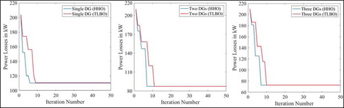
Figure 6. Comparison of objective function convergence characteristics of HHO and TLBO with type-I DG for 69-bus RDS.

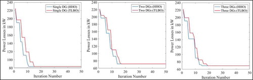
Figure 7. Bus voltages with and without Type-II DGs deployment and the effect of the number of DGs on loss minimization for 33- and 69-bus systems.

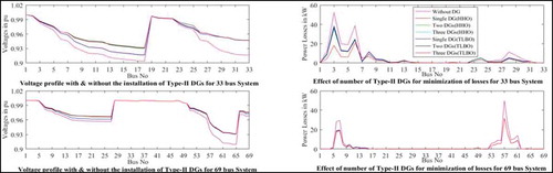
Figure 8. Comparison of objective function convergence characteristics of HHO and TLBO with type-II DG for 33-bus RDS.

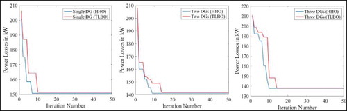
Figure 9. Comparison of objective function convergence characteristics of HHO and TLBO with type-II DG for 69-bus RDS.

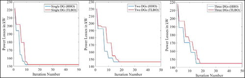
Table 4. Comparison of simulation results of HHO and TLBO type-II DG units for 69-bus system

Method	Optimal Size of DG			Total Size of DG(kVAr)	Total Active Power Losses (kW)	Total Reactive Power Losses (kVAR)	% Active Power Loss Reduction	Vmin,p.u
Single DG Unit
HHO	1328.2988(61)			1328.2988	152.041	70.5022	32.43	0.9307
TLBO	1329.951(61)			1329.951	152.041	70.5026	32.43	0.9307
HGWO (Sanjay et al., 2017)	1330(61)			1330	152.041	NA	32.43	0.9311
Hybrid (Kansal et al., 2016)	1290(61)			1290	152.1	NA	32.40	NA
2-DG Units
HHO	353.3152(17)	1280.4326(61)		1633.7478	146.44	68.2433	34.92	0.9312
TLBO	360.3115(17)	1274.4034(61)		1634.7149	146.4418	68.2399	34.91	0.9311
HGWO (Sanjay et al., 2017)	364(17)	1277(61)		1641	146.44	NA	34.92	0.9315
Hybrid (Kansal et al., 2016)	350(18)	1240(61)		1590	146.52	NA	34.88	NA
3-DG Units
HHO	318.6356(11)	285.1434(17)	1242.1248(61)	1845.9038	145.1135	67.6915	35.51	0.9314
TLBO	413.3228(11)	230.5589(21)	1232.5096(61)	1876.3913	145.1166	67.6595	35.50	0.9314
HGWO (Sanjay et al., 2017)	412(11)	230(21)	1231(61)	1873	145.115	NA	35.50	0.9317
Hybrid (Kansal et al., 2016)	330(11)	250(18)	1190(61)	1770	145.24	NA	35.45	NA
FPA (Tamilselvan et al., 2018)	450(11)	150(22)	1350(61)	1,950	145.86	NA	35.17	0.933

7.4. Scenario-4: System performance with Type-III DG integration

7.4.1. 33 bus system

Results of placing Type-III DGs by HHO and TLBO technique yields in the reduction of power loss and voltage profile which are shown in Table 5. The total power losses reduced by 67.98%, 86.49% and 94.41% for single, two and three DGs placed respectively for HHO and 67.84%, 86.47% and 94.41% for TLBO. The minimum voltage noticed was 0.9922, 0.9803 and 0.9586 p.u with three, two and single DG respectively for HHO and 0.9909, 0.9803 and 0.9582 p.u respectively for TLBO.

Table 5. Comparison of simulation results of HHO and TLBO type-III DG units for 33-bus system

Method	Optimal Size of DG in KVA			Total Size of DG(kVA)	Total Active Power Losses (kW)	Total Reactive Power Losses (kVAR)	% Active Power Loss Reduction	Vmin,p.u
Single DG Unit
HHO	3101.2881@0.82(6)			3091.2881	67.566	54.5914	67.98	0.9586
TLBO	3097.5757@0.83(6)			3097.5757	67.8579	54.833	67.84	0.9582
Dragonfly (Suresh & Belwin, 2018)	3073.5011@0.9(6)			3073.5011	70.8652	56.7703	66.41	0.9566
HGWO (Sanjay et al., 2017)	3105.9994@0.82(6)			3105.9994	67.855	NA	67.83	0.9455
Hybrid (Kansal et al., 2016)	3028.0019@0.82(6)			3028.0019	67.9	NA	67.82	NA
PSO (Kansal et al., 2016)	3034.9981@0.82(6)			3034.9981	67.9	NA	67.82	NA
HSA-PABC (Muthukumar & Jayalalitha, 2016)	3011.7035@0.85(6)			3011.7035	68.29	NA	67.63	0.9568
2-DG Units
HHO	931.2068@0.91(13)	1542.0909@0.72(30)		2473.2977	28.5047	20.3922	86.49	0.9803
TLBO	927.2892@0.89(13)	1546.3388@0.74(30)		2473.628	28.5381	20.4362	86.47	0.9803
HGWO (Sanjay et al., 2017)	932.0003@0.9(13)	1557.9989@0.72(30)		2489.9992	28.5	NA	86.49	0.9802
Hybrid (Kansal et al., 2016)	1039.0008@0.91(13)	1507.998@0.72(30)		2546.9988	28.6	NA	86.44	NA
PSO (Kansal et al., 2016)	913.9992@0.91(13)	1534.9991@0.73(30)		2448.9983	28.6	NA	86.44	NA
3-DG Units
HHO	874.3019@0.91(13)	1141.1166@0.88(24)	1456.8377@0.72(30)	3472.2562	11.7896	9.7677	94.41	0.9922
TLBO	844.0632@0.91(13)	1195.1112@0.9(24)	1446.6015@0.72(30)	3485.7759	11.7999	9.856	94.41	0.9909
HGWO (Sanjay et al., 2017)	877.9994@0.9(13)	1181.9992@0.9(24)	1454.7006@0.71(30)	3514.6992	11.74	NA	94.44	0.9922
Hybrid (Kansal et al., 2016)	872.9992@0.9(13)	1186.0004@0.89(24)	1439.0027@0.71(30)	3498.0023	11.7	NA	94.45	NA
PSO (Kansal et al., 2016)	863.0013@0.91(13)	1188.0012@0.9(24)	1430.9982@0.71(30)	3482.0007	11.8	NA	94.41	NA

7.4.2. 69-bus system

Table 6 illustrates the simulation results of placing Type-III DGs by HHO and TLBO techniques. The total power losses reduced by 89.7%, 96.82% and 98.11% for single, two and three DGs placed respectively for HHO and 89.70%, 96.80% and 98.08% for TLBO. The minimum voltage recognized was 0.9943, 0.9943 and 0.9725 p.u with three, two and single DG respectively for HHO and 0.9943, 0.9935 and 0.9725 p.u for TLBO. Figure 10 shows the bus voltages with and without type-III DGs deployment and the effect of the number of DGs on loss minimization for 33- and 69-bus systems. The convergence characteristic curves of the proposed HHO and TLBO algorithms for optimal placement and sizing of type-III DGs are shown in Figures 11 and 12 for 33- and 69-bus RDS respectively.

Figure 10. Bus voltages with and without Type-III DGs deployment and the effect of the number of DGs on loss minimization for 33 and 69-bus systems.

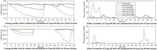
Figure 11. Comparison of objective function convergence characteristics of HHO and TLBO with type-III DG for 33-bus RDS.

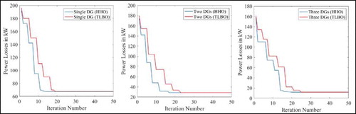
Figure 12. Comparison of objective function convergence characteristics of HHO and TLBO with type-III DG for 69-bus RDS.

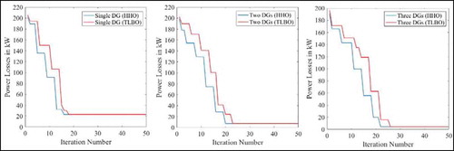
Table 6. Comparison of simulation results of HHO and TLBO type-III DG units for 69-bus system

Method	Optimal Size of DG in kVA			Total Size of DG(kVA)	Total Active Power Losses (kW)	Total Reactive Power Losses (kVAR)	% Active Power Loss Reduction	Vmin, p.u
Single DG Unit
HHO	2243.0817@0.81(61)			2233.0817	23.1704	14.3799	89.70	0.9725
TLBO	2238.0394@0.81(61)			2238.0394	23.1719	14.3741	89.70	0.9725
EHO (Prasad et al., 2019)	2216.2988@0.9(61)			2216.2988	27.95	16.46	87.58	0.9724
Dragonfly (Suresh & Belwin, 2018)	2217.3006@0.9(61)			2217.3006	27.9636	16.4979	87.57	0.9728
HGWO (Sanjay et al., 2017)	2245.9991@0.81(61)			2245.9991	23.16	NA	89.71	0.9724
Hybrid (Kansal et al., 2016)	2239.9983@0.81(61)			2239.9983	23.19	NA	89.69	NA
PSO (Kansal et al., 2016)	2219.9975@0.81(61)			2219.9975	23.2	NA	89.69	NA
2-DG Units
HHO	591.5419@0.85	1751.6811@0.98(61)		2343.223	7.1579	8.0652	96.82	0.9943
TLBO	588.5816@0.83	1755.482@0.98(61)		2344.0636	7.21	8.1366	96.8	0.9935
HGWO (Sanjay et al., 2017)	627.9975@0.82	1759.9654@0.98(61)		2387.9629	7.2	NA	96.8	0.9941
Hybrid (Kansal et al., 2016)	630.0006@0.82	1754.6512@0.98(61)		2384.6518	7.21	NA	96.8	NA
PSO (Kansal et al., 2016)	630.0006@0.82	1762.5791@0.98(61)		2392.5797	7.2	NA	96.8	NA
3-DG Units
HHO	594.7508@0.6(11)	461.9811@0.9(18)	2051.6078@0.82(61)	3108.3397	4.26	6.86	98.11	0.9943
TLBO	575.7381@0.84(11)	478.005@0.79(18)	2054.8594@0.82(61)	3108.6025	4.33	6.7863	98.08	0.9943
HGWO (Sanjay et al., 2017)	614.0012@0.81(11)	452.0005@0.83(18)	2055.9942@0.81(61)	3121.9959	4.26	NA	98.11	0.9942
Hybrid (Kansal et al., 2016)	479.9993@0.7(18)	2059.9986@0.83(61)	529.9985@0.82(66)	3069.9964	4.3	NA	98.09	NA
PSO (Kansal et al., 2016)	600.0011@0.83(11)	460.0013@0.81(18)	2060.0026@0.81(61)	3120.005	4.61	NA	97.95	NA

7.5. Scenario-5: System performance with Type-IV DG integration

7.5.1. 33-bus system

Results of placing Type-IV DGs by HHO and TLBO technique yields in the reduction of power loss, better voltage profile and improved savings which are shown in Table 7. The total power losses reduced by 27.58%, 33.68% and 38.41% for single, two and three DGs placed respectively for HHO and 27.37%, 33.59% and 38.32% for TLBO. The least voltage noticed was 0.9424, 0.9419 and 0.9265 p.u with three, two and single DG respectively for HHO and 0.9423, 0.9418 and 0.9263 p.u for TLBO.

Table 7. Comparison of simulation results of HHO and TLBO type-IV DG units for 33-bus system

Method	Optimal Size of DG(kW)	Optimal Size of DG(kVAR)	Optimal Location	Total Active Power Losses (kW)	Total Reactive Power Losses (kVAR)	% Active Power Loss Reduction	Vmin,p.u
Single DG
HHO	1869.5848	583.6843	6	152.7911	107.4204	27.58	0.9265
TLBO	1874.4215	585.1944	6	153.2342	107.7698	27.37	0.9263
Analytical (Kansal et al., 2011)	1520	592	12	163.3	113.7	22.60	NA
PSO (Kansal et al., 2011)	2180	691	12	155.3	109.4	26.39	NA
2-DG Units
HHO	661.4236 & 752.6153	206.4964 & 234.9664	13,30	139.932	95.0844	33.68	0.9419
TLBO	663.3723 & 756.0958	207.1048 & 236.0531	13,30	140.1248	95.236	33.59	0.9418
3-DG Units
HHO	621.783, 861.8085 & 679.52	194.1206, 269.0566 & 212.1461	13, 24 & 30	129.9439	88.7636	38.41	0.9424
TLBO	626.7492, 860.5756 & 678.7221	195.6711, 268.6717 & 211.897	13, 24 & 30	130.1358	88.9056	38.32	0.9423

7.5.2. 69-bus system

Table 8 illustrates the simulation results of placing Type-IV DGs by HHO and TLBO techniques. The total power losses reduced by 37.18%, 40.24% and 40.88% for single, two and three DGs placed respectively for HHO and 37.10%, 40.20% and 40.64% for TLBO. The minimum voltage detected was 0.9540, 0.9540 and 0.9539 with three, two and single DG respectively for HHO and 0.9540, 0.9540 and 0.9539 p.u for TLBO. Figure 13 shows the bus voltages with and without type-IV DGs deployment and the effect of the number of DGs on loss minimization for 33 and 69-bus systems. The convergence characteristic curves of the proposed HHO and TLBO algorithms for optimal placement and sizing of type-IV DGs are shown in Figures 14 and 15 for 33 and 69-bus RDS respectively.

Figure 13. Bus voltages with and without Type-IV DGs deployment and the effect of the number of DGs on loss minimization for 33 and 69-bus systems.

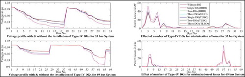
Figure 14. Comparison of objective function convergence characteristics of HHO and TLBO with type-IV DG for 33-bus RDS.

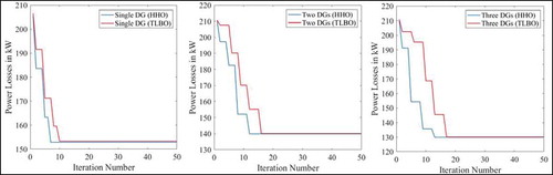
Figure 15. Comparison of objective function convergence characteristics of HHO and TLBO with type-IV DG for 69-bus RDS.

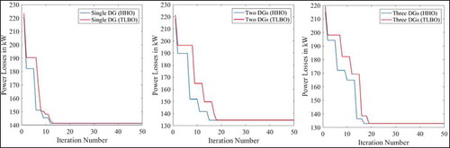
Table 8. Comparison of simulation results of HHO and TLBO type-IV DG units for 69-bus system

Method	Optimal Size of DG(kVA)	Optimal Size of DG(kVAR)	Optimal Location	Total Active Power Losses (kW)	Total Reactive Power Losses (kVAR)	% Active Power Loss Reduction	Vmin,p.u
Single DG Unit
HHO	1363.6773	425.74	61	141.3448	65.9110	37.18	0.9539
TLBO	1364.0648	425.861	61	141.5253	65.9114	37.10	0.9539
DPSO (Musa et al., 2016)	1500	658.9	61	169.4	NA	24.71	0.9548
Analytical (Kansal et al., 2011)	1360	574	56	199	89.5	11.56	NA
PSO (Kansal et al., 2011)	1720	618	56	193.4	86.5	14.04	NA
2-DG Units
HHO	389.1711 & 1301.077	121.4992 & 406.1962	17 & 61	134.4672	63.1246	40.24	0.9540
TLBO	389.8568 & 1302.6048	121.7133 & 406.6732	17 & 61	134.5546	63.1247	40.20	0.9540
DPSO (Musa et al., 2016)	600 & 843	280.7 & 400.1	11 & 61	165.1	NA	26.62	0.9379
3-DG Units
HHO	357.1266, 293.4857 & 1262.3744	111.4949, 91.6262 & 394.1132	11,17 & 61	133.0089	62.3015	40.88	0.9540
TLBO	396.7555, 279.2014 & 1255.2844	123.867, 87.1667 & 391.8997	11,17 & 61	133.0914	62.4897	40.64	0.9540

7.6. Scenario-6: Economical analysis with DG integration

7.6.1. 33-bus system

The cost of energy losses, cost of active and reactive power supplied by DG are shown in Table 9. The cost of energy losses without DG are 16983.49$ and are reduced to 8871.70$, 7014.17$ and 5853.45$ by using HHO algorithm, and they are reduced to 8911.30$, 7015.18$ and 5857.65$ by using TLBO algorithm when single, two and three Type-I DGs are installed respectively. With the integration of single, two and three type-II DGs, the cost of energy losses are reduced to 12,125.66$, 11359.70$ and 11085.07$ when using HHO algorithm and are reduced to 12184.15$, 11416.62$ and 11128.69$ when using TLBO algorithm. The cost of energy losses is reduced to 5438.74$, 2294.49$ and 949.01$ by using HHO algorithm, and they are reduced to 5462.24$, 2297.18$ and 949.84$ by using TLBO algorithm with the incorporation of single, two and three Type-III DGs respectively. With the application of single, two and three type-IV DGs, the cost of energy losses is decreased to 14,263.26$, 13,689.72$ and 13,140.48$ by using HHO algorithm and are reduced to 14,307.02$, 13,717.61$ and 13,168.22$ by using TLBO algorithm.

Table 9. Comparison of economic analysis of HHO and TLBO for 33-bus system

Type-I DG
Description	Single DG Unit		Two DG Units		Three DG Units
	HHO	TLBO	HHO	TLBO	HHO	TLBO
Cost of energy losses ($)	8871.70	8911.30	7014.17	7015.18	5853.45	5857.65
Cost of active power supplied by DG ($/MWh)	51.93	51.94	40.29	40.31	58.44	59.10
Type-II DG
Descrip tion	Single DG Unit		Two DG Units		Three DG Units
	HHO	TLBO	HHO	TLBO	HHO	TLBO
Cost of energy losses ($)	12125.66	12184.15	11359.70	11416.62	11085.07	11128.69
Cost of reactive power supplied by DG ($/MVARh)	25.40	25.41	30.82	30.83	39.22	39.60
Type-III DG
Descrip tion	Single DG Unit		Two DG Units		Three DG Units
	HHO	TLBO	HHO	TLBO	HHO	TLBO
Cost of energy losses ($)	5438.74	5462.24	2294.49	2297.18	949.01	949.84
Cost of active power supplied by DG ($/MWh)	50.95	51.67	39.65	39.89	57.72	58.46
Cost of reactive power supplied by DG ($/MVARh)	9.93	9.41	9.11	8.94	11.06	10.65
Type-IV DG
Descrip tion	Single DG Unit		Two DG Units		Three DG Units
	HHO	TLBO	HHO	TLBO	HHO	TLBO
Cost of energy losses ($)	14263.26	14,307.02	13689.72	13717.61	13140.48	13168.22
Cost of active power supplied by DG ($/MWh)	40.09	40.23	29.61	29.74	47.01	47.13

7.6.2. 69-bus system

Table 10 illustrates the cost of energy losses, the cost of active and reactive power supplied by DG. The cost of energy losses without DG is 18,111.42$. With the integration of single, two and three type-I DGs and application of HHO algorithm, the cost of energy losses is reduced to 6697.52$, 5769.66$ and 5588.86$, and with the application of TLBO, they are reduced to 6699.13$, 5769.66$ and 5588.87$. The cost of energy losses is decreased to 12238.61$, 11787.72$ and 11680.94$ by using HHO algorithm and reduced to 12238.57$, 11787.86$ and 11681.19$ by using TLBO algorithm when single, two and three Type-II DGs are installed respectively. By using HHO algorithm, the cost of energy losses is reduced to 1865.11$, 576.18$ and 342.91$, and by application of TLBO algorithm, they are reduced to 1865.23$, 580.37$ and 348.54$ with the incorporation of single, two and three Type-III DGs respectively. With the application of single, two and three type-IV DGs, the cost of energy losses is decreased to 14183.27$, 13848.64$ and 13773.78$ by using HHO algorithm and are reduced to 14184.32$, 13848.64$ and 13774.98$ by using TLBO algorithm.

Table 10. Comparison of economic analysis of HHO and TLBO for 69-bus system

Type-I DG
Description	Single DG Unit		Two DG Units		Three DG Units
	HHO	TLBO	HHO	TLBO	HHO	TLBO
Cost of energy losses ($)	6697.52	6699.13	5769.66	5769.66	5588.86	5588.87
Cost of active power supplied by DG ($/MWh)	37.70	37.70	46.51	46.52	52.87	52.93
Type-II DG
Descrip tion	Single DG Unit		Two DG Units		Three DG Units
	HHO	TLBO	HHO	TLBO	HHO	TLBO
Cost of energy losses ($)	12238.61	12238.57	11787.72	11787.86	11,680.94	11681.19
Cost of reactive power supplied by DG ($/MVARh)	26.84	26.85	32.92	32.94	37.17	37.78
Type-III DG
Descrip tion	Single DG Unit		Two DG Units		Three DG Units
	HHO	TLBO	HHO	TLBO	HHO	TLBO
Cost of energy losses ($)	1865.11	1865.23	576.18	580.37	342.91	348.54
Cost of active power supplied by DG ($/MWh)	36.43	36.51	46.61	44.68	49.85	51.67
Cost of reactive power supplied by DG ($/MVARh)	7.56	7.58	2.50	2.43	11.53	10.03
Type-IV DG
Descrip tion	Single DG Unit		Two DG Units		Three DG Units
	HHO	TLBO	HHO	TLBO	HHO	TLBO
Cost of energy losses ($)	14183.27	14184.32	13848.64	13848.64	13773.78	13774.98
Cost of active power supplied by DG ($/MWh)	29.51	29.51	36.61	36.61	41.92	41.93

8. Conclusions

Harries Hawks Optimization and Teaching Learning-Based Optimization algorithms for optimum location and size of different types of DGs in distribution networks have been proposed. It seeks to maximize technical and financial upsides. Five operational scenarios were applied and compared to other optimization techniques on two distribution test systems.

The major findings of the simulation are summarized as follows.

1) The optimum placement and sizing of the three type-III DGs have led to a major reduction in power losses of 11.7896 kW and 11.7999 kW for 33-bus system where as they are 4.26 kW and 4.33 kW for 69-bus system using HHO and TLBO techniques respectively.

2) The minimum cost of energy losses is 949.01 USD and 949.84 USD for 33-bus system whereas it is 342.91 USD and 348.54 USD for 69-bus system using HHO and TLBO techniques respectively when three Type-III DG units are installed.

3) It is observed that HHO exhibits fast convergence characteristics in comparison to TLBO.

By observing the above major findings, it can be concluded that the performance of HHO algorithm is superior when compared with TLBO and other algorithms exist in literature to determine the optimal size and placement of DG.

In future research work, the optimization problem could be extended to investigate on three-phase unbalanced radial distribution systems. The optimization can be carried out for a hybrid DG system with multiple DG units along with the battery. In addition, the influence of the intermittent nature of renewable DG could be addressed based on uncertainty modeling.

Nomenclature

The main notation used in the text is listed below, sorted alphabetically. Other symbols and abbreviations are defined where they appear.

Table

Ii	Current flowing in the i^th branch
K	No of DGs
Kel	Yearly cost of energy loss ($/kWh)
Kpl	Yearly demand cost of power loss ($/kW)
Lf	Load factor
Lsf	Loss factor
n	No. of branches
Pd	Active power demand connected to the system
Pdg	Total active power supplied by DGs
PL	Total active power losses of the system
Psupply	Active power supplied by the main feeder
PGk	Active power generated by DG at k^th bus
$P{G}_k^{min}$	Minimum allowed output active power of DG unit at k^th bus
$P{G}_k^{max}$	Maximum allowed output active power of DG unit at k^th bus
Qd	Reactive power demand connected to the system
Qdg	Total reactive power supplied by DGs
QL	Total reactive power losses of the system
Qsupply	Reactive power supplied by the main feeder
QGk	Reactive power generated by DG at k^th bus
$Q{G}_k^{min}$	Minimum allowed output reactive power of DG unit at k^th bus
$Q{G}_k^{max}$	Maximum allowed output reactive power of DG unit at k^th bus
Ri	Resistance of the i^th branch
$S{L}_k$	Loading at k^th bus
$S{L}_k^{max}$	Maximum allowed Loading at k^th bus
$T_k$	Tap setting of transformer at k^th bus
$T_k^{min}$	Minimum allowed tap setting of transformer at k^th bus
$T_k^{max}$	Maximum allowed tap setting of transformer at k^th bus
VGk	Generator Voltage at k^th bus
VLk	Load Voltage at k^th bus
$V{L}_k^{min}$	Minimum allowed load Voltage at k^th bus
$V{L}_k^{max}$	Maximum allowed load Voltage at k^th bus

Additional information

Funding

The authors received no direct funding for this research.

Notes on contributors

Ponnam Venkata K. Babu

Ponnam Venkata K. Babu is presently working as an Assistant Professor in the Department of Electrical & Electronics Engineering at RVR&JC College of Engineering, Guntur. He Completed B.Tech (Electrical and Electronics Engineering) in 2002 from Narasaraopeta Engineering College, Narasaraopeta, Guntur, India, and MTech (Power Systems Engineering) in 2013 from RVR&JC College of Engineering, Guntur, India. Currently he is pursuing PhD in Acharya Nagarjuna University, Guntur, India. His research interests are in the areas of power systems, AI Techniques and Soft Computing Techniques, etc.

K. Swarnasri

K. Swarnasri is presently working as Professor in Department of Electrical & Electronics Engineering at RVR&JC College of Engineering, Guntur. She has Completed her BTech (EEE) in 1999 from RVR&JC College of Engineering and MTech (Power Systems Engineering) in 2001 from REC-Warangal. She obtained her PhD degree from JNTU-Hyderabad in 2014. Her research interests are in the areas of electrical power systems, power quality, energy audit and conservation, renewable energy, smart grids, AI techniques, etc.

References

- Babu, P. V. K., Swarnasri, K., & Vijetha, P. (2018). A three phase unbalanced power flow method for secondary distribution system. Advance Modeling Analysis B, 61(3), 139-144. https://doi.org/10.18280/ama_b.610306
- Carpinelli, G., Celli, G., Pilo, F., & Russo, A. 2001. Distributed generation siting and sizing under uncertainty. 2001 IEEE Porto Power Tech proceedings (Cat. no.01EX502) (Vol. 4, pp. 7). Porto, Portugal. https://doi.org/10.1109/PTC.2001.964856
- ChithraDevi, S. A., Lakshminarasimman, L., & Balamurugan, R. (2017). Stud Krill herd algorithm for multiple DG placement and sizing in a radial distribution system. Engineering Science and Technology, 20(2), 748–36. https://doi.org/10.1016/j.jestch.2016.11.009
- Eroshenko, S. A., Khalyasmaa, A. I., Dmitriev, S. A., Pazderin, A. V., & Karpenko, A. A. 2013. Distributed generation siting and sizing with implementation feasibility analysis. 2013 international conference on power, energy and control (ICPEC) (pp. 717–721). Sri Rangalatchum Dindigul. https://doi.org/10.1109/ICPEC.2013.6527749
- Heidari, A. A., Mirjalili, S., Faris, H., Aljarah, I., Mafarja, M., & Chen, H. (2019). Harris hawks optimization: Algorithm and applications. Future Generation Computer Systems, 97, 849–872. https://doi.org/10.1016/j.future.2019.02.028
- Imran Ahmad Quadri, S., & Bhowmick, D. J. (2018). A comprehensive technique for optimal allocation of distributed energy resources in radial distribution systems. Applied Energy, 211, 1245–1260. https://doi.org/10.1016/j.apenergy.2017.11.108
- Kansal, S., Sai, B. B. R., Tyagi, B., & Kumar, V. 2011. Optimal placement of wind-based generation in distribution networks. IET conference on renewable power generation (RPG 2011) (pp. 1–6). Edinburgh. https://doi.org/10.1049/cp.2011.0141
- Kansal, S., Kumar, V., & Tyagi, B. (2013). Optimal placement of different type of DG sources in distribution networks. International Journal of Electrical Power & Energy Systems, 53, 752–760. https://doi.org/10.1016/j.ijepes.2013.05.040
- Kansal, S., Kumar, V., & Tyagi, B. (2016). Hybrid approach for optimal placement of multiple DGs of multiple types in distribution networks. International Journal of Electrical Power & Energy Systems, 75, 226–235. https://doi.org/10.1016/j.ijepes.2015.09.002
- Kaur, S., Kumbhar, G., & Sharma, J. (2014). A MINLP technique for optimal placement of multiple DG units in distribution systems. International Journal of Electrical Power & Energy Systems, 63, 609–617. https://doi.org/10.1016/j.ijepes.2014.06.023
- Kayalvizhi, S., & Vinod Kumar, D. M. (2018). Optimal planning of active distribution networks with hybrid distributed energy resources using grid-based multi-objective harmony search algorithm. Applied Soft Computing, 67, 387–398. https://doi.org/10.1016/j.asoc.2018.03.009
- Khosravi, S., Zamanifar, M., & Derakhshan-Barjoei, P. (2018). Analysis of bifurcations in a wind turbine system based on DFIG. Emerging Science Journal, 2(1), 39–52. https://doi.org/10.28991/esj-2018-01126
- Loong, L. H., Sabev, V. P., & Jaromír, K. J. (2011). Regional renewable energy and resource planning. Applied Energy, 88(2), 545–550. https://doi.org/10.1016/j.apenergy.2010.05.019
- Malekpour, A. R., Niknam, T., Pahwa, A., & Kavousi Fard, A. (2013, May). Multi-objective stochastic distribution feeder reconfiguration in systems with wind power generators and fuel cells using the point estimate method. IEEE Transactions on Power Systems, 28(2), 1483–1492. https://doi.org/10.1109/TPWRS.2012.2218261
- Mehdi Hosseini, S. (2018). The operation and model of UPQC in voltage sag mitigation using EMTP by direct method. Emerging Science Journal, 2(3), 148–156. https://doi.org/10.28991/esj-2018-01138
- Mohamed Imran, A., & Kowsalya, M. (2014). Optimal size and siting of multiple distributed generators in distribution system using bacterial foraging optimization. Swarm and Evolutionary Computation, 15, 58–65. https://doi.org/10.1016/j.swevo.2013.12.001
- Mohsen, M., Youssef, A., Ebeed, M., & Kamel, S. 2017. Optimal planning of renewable distributed generation in distribution systems using grey wolf optimizer GWO. 2017 nineteenth international Middle East power systems conference (MEPCON) (pp. 915–921). Cairo. https://doi.org/10.1109/MEPCON.2017.8301289
- Mokryani, G., & Siano, P. (2013). Optimal wind turbines placement within a distribution market environment. Applied Soft Computing, 13(10), 4038–4046. https://doi.org/10.1016/j.asoc.2013.05.019
- Moravej, Z., & Akhlaghi, A. (2013). A novel approach based on cuckoo search for DG allocation in distribution network. International Journal of Electrical Power & Energy Systems, 44(1), 672–679. https://doi.org/10.1016/j.ijepes.2012.08.009
- Murthy, V. V. S. N., & Kumar, A. (2013). Comparison of optimal DG allocation methods in radial distribution systems based on sensitivity approaches. International Journal of Electrical Power & Energy Systems, 53, 450–467. https://doi.org/10.1016/j.ijepes.2013.05.018
- Murty, V. V. V. S. N., & Kumar, A. (2019). Optimal DG integration and network reconfiguration in microgrid system with realistic time varying load model using hybrid optimisation. IET Smart Grid, 2(2), 192–202. https://doi.org/10.1049/iet-stg.2018.0146
- Musa, I., Gadoue, S., & Zahawi, B. (2016). Integration of induction generator based distributed generation in power distribution networks using a discrete particle swarm optimization algorithm. Electric Power Components and Systems, 44(3), 268–277. https://doi.org/10.1080/15325008.2015.1110215
- Muthukumar, K., & Jayalalitha, S. (2016). Optimal placement and sizing of distributed generators and shunt capacitors for power loss minimization in radial distribution networks using hybrid heuristic search optimization technique. International Journal of Electrical Power & Energy Systems, 78, 299–319. https://doi.org/10.1016/j.ijepes.2015.11.019
- Nasiraghdam, H., & Jadid, S. (2012). Optimal hybrid PV/WT/FC sizing and distribution system reconfiguration using multi-objective artificial bee colony (MOABC) algorithm. Solar Energy, 86(10), 3057–3071. https://doi.org/10.1016/j.solener.2012.07.014
- Niknam, T., Bornapour, M., & Gheisari, A. (2013). Combined heat, power and hydrogen production optimal planning of fuel cell power plants in distribution networks. Energy Conversion and Management, 66, 11–25. https://doi.org/10.1016/j.enconman.2012.08.016
- Niknam, T., Taheri, S. I., Aghaei, J., Tabatabaei, S., & Nayeripour, M. (2011). A modified honey bee mating optimization algorithm for multiobjective placement of renewable energy resources. Applied Energy, 88(12), 4817–4830. https://doi.org/10.1016/j.apenergy.2011.06.023
- Paterakis, N. G., Mazza, A., Santos, S. F., Erdinc, O., Chicco, G., Bakirtzis, A. G., & Catalao, J. P. S. (2016). Multi-objective reconfiguration of radial distribution systems using reliability indices. IEEE Transactions on Power Systems, 31(2), 1048–1062. https://doi.org/10.1109/TPWRS.2015.2425801
- Pazouki, S., Mohsenzadeh, A., Ardalan, S., & Haghifam, M. (2016). Optimal place, size, and operation of combined heat and power in multi carrier energy networks considering network reliability, power loss, and voltage profile. IET Generation, Transmission & Distribution, 10(7), 1615–1621. https://doi.org/10.1049/iet-gtd.2015.0888
- Prakash, D. B., & Lakshminarayana, C. (2018). Multiple DG placements in radial distribution system for multi objectives using whale optimization algorithm. Alexandria Engineering Journal, 57(4), 2797–28065. https://doi.org/10.1016/j.aej.2017.11.003
- Prasad, C. H., Subbaramaiah, K., & Sujatha, P. (2019). Cost–benefit analysis for optimal DG placement in distribution systems by using elephant herding optimization algorithm. Renewables: Wind, Water and Solar, 6(1). https://doi.org/10.1186/s40807-019-0056-9
- Rao, R. V., Savsani, V. J., & Vakharia, D. P. (2011). Teaching learning-based optimization: A novel method for constrained mechanical design optimization problems. Computer Aided Design, 43(3), 303–315. https://doi.org/10.1016/j.cad.2010.12.015
- Sanjay, R., Jayabarathi, T., Raghunathan, T., Ramesh, V., & Mithulananthan, N. (2017). Optimal allocation of distributed generation using hybrid Grey Wolf optimizer. IEEE Access, 5, 14807–14818. https://doi.org/10.1109/ACCESS.2017.2726586
- Sheen, J.-N., Tsai, M.-T., & Wu, S.-W. (2013). A benefits analysis for wind turbine allocation in a power distribution system. Energy Conversion and Management, 68, 305–312. https://doi.org/10.1016/j.enconman.2012.12.022
- Sheng, W., Liu, K., Liu, Y., Meng, X., & Li, Y. (2015, April). Optimal placement and sizing of distributed generation via an improved nondominated sorting genetic algorithm II. IEEE Transactions on Power Delivery, 30(2), 569–578. https://doi.org/10.1109/TPWRD.2014.2325938
- Singh, R. K., & Goswami, S. K. (2009). Optimum siting and sizing of distributed generations in radial and networked systems. Electric Power Components and Systems, 37(2), 127–145. https://doi.org/10.1080/15325000802388633
- Sulaiman, M. H., Mustafa, M. W., Azmi, A., Aliman, O., & Abdul Rahim, S. R. 2012. Optimal allocation and sizing of distributed generation in distribution system via firefly algorithm. 2012 IEEE international power engineering and optimization conference Melaka, Malaysia (pp. 84–89). Melaka. https://doi.org/10.1109/PEOCO.2012.6230840
- Suresh, M. C. V., & Belwin, E. J. (2018). Optimal DG placement for benefit maximization in distribution networks by using Dragonfly algorithm. Renewables: Wind, Water and Solar, 5(1), 4. https://doi.org/10.1186/s40807-018-0050-7
- Tamilselvan, V., Jayabarathi, T., Raghunathan, T., & Yang, X.-S. (2018). Optimal capacitor placement in radial distribution systems using flower pollination algorithm. Alexandria Engineering Journal, 57(4), 2775–2786. https://doi.org/10.1016/j.aej.2018.01.004