Calculation of road profiles by reversing the solution of the vertical ride dynamics forward problem

Abstract

Road profiles are an important input into vehicle simulation studies and a key part of road surface condition. However, their availability is often limited by the insufficient existence of simpler road profiling procedures. Therefore, the main purpose of this paper is to present a simple analytical procedure for the calculation of road profiles from given or measured vehicle accelerations. In the paper, an analytical procedure is derived based on a quarter car ride model, which uses accelerations obtained from sprung mass only, unsprung mass only and both sprung and unsprung masses to inversely calculate road profiles. The performance of the approach is demonstrated through a numerical and experimental study at different vehicle speeds, for different suspension settings, under various levels of noise and for a nonlinear LuGre damping model. The developed procedure produces very good results at lower vehicle speeds and it is further shown to produce correlations of above 97% with actual profiles when both the actual and reconstructed profiles are low-pass filtered at a cut-off frequency of one-third of the sprung mass resonance. The need for system characterisation makes this procedure suitable for use with light vehicles. Furthermore, its speed limitations make it suitable for application on township or suburb roads, or unpaved rough terrains where low speeds are often recommended.

Keywords:

• road profile reconstruction
• quarter car model
• Runge-Kutta numerical integration
• transmissibility ratio
• LuGre damping model
• inertial profiling systems

PUBLIC INTEREST STATEMENT

This paper presents a methodology for determining road surface profiles from accelerations that are measured through a smartphone firmly fixed to the passenger cabin (under the rear passenger’s seat). This position was selected because it was relatively more accessible and safe for instrumentation for the specific vehicle that used in the study. This is an extremely simple technique, which is ideal for use on rural and semi-urban road networks where deployment of modern road profiling systems is hard due to their high demand on the urban roads. This methodology involves identification of a quarter-car model parameters for a particular vehicle which are then applied to an algorithm that calculates the road surface profiles upon receiving acceleration inputs. In this study, the technique is successfully demonstrated through tests over a speed bump and through a number of numerical investigations under different vehicle operating conditions.

1. Introduction

Since the early 1980s road maintenance has become a focus for many municipalities around the world. Many municipalities have spent millions of dollars towards road maintenance and repairs. For example, the German government spent well in excess of 10 billion euros in 2015 on road maintenance projects while US spent an estimated 182 billion dollars on capital improvements and maintenance of federal highways in 2008 (Schnebele et al., 2015). These figures are likely to have increased over the years with the demands of smart cities where traffic management and road maintenance have become of utmost importance. However, it is expected that the increase in these figures can be under control with early detection of road damage and timely implementation of road maintenance actions.

Road surface condition is a key indicator of road quality and measurements of road roughness are often used by road agencies to assess road surface conditions. The determination of road roughness level solely relies on measurement of road profiles. Patterson (Paterson, 1987) shows that road roughness impacts on a number of vehicle-road-related aspects such as vehicle dynamics, wear of vehicle parts, vehicle operating costs, safety, and speed of travel. Road roughness increases the dynamic loadings imposed by vehicles on the road surface thereby accelerating the rates of deterioration of the pavement structure (Directorate for Science, Technology and Industry (DSTI), 1998). The cost of operating the vehicles and transporting goods rises as road roughness increases and as the total operating costs of all vehicles on a road outweigh the agency costs of maintaining the road by typically 10- to 20-fold, thus small improvements in road roughness can yield high economic returns (Paterson, 1987). In order for engineers to determine road roughness level, predict road damage, design optimal suspension systems, predict fatigue damage to vehicle parts and determine the fuel efficiency, there is need either to perform real-life tests on the roads or measure the road profiles for specific roads and simulate them under laboratory testing. Due to cost implications resulting from real-life testing and laboratory testing, computer simulations are a desirable alternative. Besides, the current availability of high-performance supercomputers at affordable computing costs, has made the use of computer simulations a more feasible approach.

However, the use of computer simulations for this type of work does not negate the importance of obtaining real road surface profiles. Therefore, there is always the need to measure the road profiles. Road profiles are typically measured using two different types of measurement systems: systems that directly measure road profiles and those that estimate road profiles from the dynamic responses of a moving vehicle (Sayers et al., 1986; Sayers & Karamihas, 1998). The first type of systems employs geotechnical methods and often static in nature. Though they provide more accurate measurements, which are typically used for calibrating other systems, their application on very long and high-volume traffic road networks can be limited. Becker and Els (Becker & Els, 2014) give a very comprehensive review of these profiling methods. The second type of measurement systems provides a more feasible option for high-speed roughness measurements since they can be designed to operate at highway speeds. These systems can be grouped into two categories: response-type road roughness measurement (RTRRM) systems and inertial profiling systems (Sayers et al., 1986; Sayers & Karamihas, 1998). RTRRM systems are based on measurements of suspension travel, and some of the popular brands include the Mays Ride Meter, the PCA meter, the Cox meter, and the Bureau of Public Roads roughometer (Sayers et al., 1986; Sayers & Karamihas, 1998). RTRRM systems have advantages of being low-cost, simple in operation, capable of measuring at high speeds with disadvantages of being vehicle property-dependent, time unstable, hard to calibrate and correlate with other systems. An analysis of the response characteristics of different road meter systems shows that they respond differently to different ranges of the road roughness spectrum (Sayers et al., 1986), thus making their measurements correlate poorly across different systems. This problem is further complicated by the differences in response characteristics of the host vehicles themselves. The systems are also subjected to many errors emanating from suspension damping, tyre pressure, wheel non-uniformities, and vehicle weight changes (Sayers et al., 1986).

Inertial profilers comprise transducers that measure accelerations in the direction of vehicle ride, sensor height positions, and a longitudinal distance along the road often measured from a reference point. The acceleration data are integrated twice to calculate the vehicle vertical displacement, which are subtracted from the sensor height data to obtain the road surface profile. A popular example of this profiler is the GMR profiler developed by Kelley and Spangler (Sayers et al., 1986). The present study is based on these systems with the exception that the height measurement is not required. However, it requires knowledge of system parameters such as sprung and unsprung masses, suspension stiffness and damping coefficients and tyre stiffness. The advantage of this approach is that the system is directly mounted on the vehicle body and does not require other cumbersome fixtures. This approach may also be beneficial to the development of autonomous vehicles where some vehicle system characteristics (e.g., suspension stiffness and tyre pressures) can be automatically adjusted in response to road conditions. This can help to improve fatigue endurance of both vehicle structure and road infrastructure owing to reduction in the resultant dynamic tyre forces.

2. Review of inertial profiling systems

There are two important developments of inertial profiling systems: those with dedicated transducers mounted directly on the vehicle axle or chassis and those that are custom-instrumented. The former may either come as part of the on-board vehicle information systems whose primary intention is to optimise various aspects of vehicle performance. The fact that these sensors are originally intended for other purposes may make their application to road condition monitoring very difficult. For example, the sensors may operate at dynamic ranges outside the desired ranges for road condition monitoring or the measured data may be sampled at inappropriate rates, or located at unsuitable positions for road condition monitoring. Their advantages include no/minimal need for extra instrumentation, data storage and power back-up units. On the other hand, the user has control over sampling rates, sensor types, and sensor locations in the custom-instrumented sensors. However, this requires data logging systems besides the processing algorithms and data transmission systems. All in all, the need for instrumentation on these systems may render them unpopular, especially to vehicle owners and manufacturers, due to the need for modification of certain vehicle parts when mounting them on the vehicles.

The most common versions of these systems involve the use of accelerations, sensor height and GPS coordinate data to calculate road profiles. Researchers have used various modelling approaches in profile reconstruction ranging from mechanistic procedures (Gonzalez et al., 2008; Hugo et al., 2008; Kropac & Mucka, 2008; Pesterev et al., 2004, 2005) to artificial intelligence models (Ngwangwa et al., 2014, 2010; Yousefzadeh et al., 2010). Some of the most recent developments have incorporated microcontroller modules such as Raspberry Pi (Celaya-Padilla et al., 2018) and Arduino (Bidgoli et al., 2019) for onboard signal processing, profile calculation and data transmission to enable real-time road condition monitoring.

Modern versions of these systems are actually very complex and opulent often using dedicated vehicles that are instrumented with cameras, laser scanners, accelerometers, gyros, GPS navigation sensors, tachometers, data acquisition systems, power supply and back-up units, and data handling and transmission systems (“ROMDAS system, 2018”; “Value of asset preservation”), among many others in different countries. These systems are capable of producing three-dimensional profiles of roads at highway speeds (up to 120 km/h) without interruption to traffic flow and are capable of conducting frequent road condition monitoring surveys. The downside of these systems is the high overhead cost, and high operating costs due to energy, data storage and transmission costs. As a result, these systems are often deployed on national highways and not on public rural roads. These public rural roads though neglected in many respects do connect rural communities to industry, markets, education, healthy and many other essential social amenities.

Therefore, low-cost alternatives that can be applied to these public rural roads have become a central focus of current research efforts. There are quite a number of these systems that are developed and reported in the literature with most of them equipped with transducers that capture vehicle responses, and algorithms that calculate road condition statistics. Some of most popular of these systems are the MIT CarTel (Hull et al., 2006), Microsoft Research NeriCell (Mohan et al., 2008), and Roadroid (Roadroid, 2019). These systems adopt a continuous sensing approach in which data is continuously sampled for all cars on all street segments and then processed offline on the back-end servers. However, Rahman et al. (Rahman et al., 2018) argue that these systems are too expensive due to their high energy demands on mobile devices.

Therefore, a number of smartphone-based systems are currently being developed as popularised by the widespread use of smartphones worldwide. Currently, smartphones come with accelerometers, gyroscopes and GPS sensors that can be used to measure vibrations in all three axes, geographical positioning, gyroscopic motions and have storage capability besides the well-known transmission capability. The systems are therefore preferred for their simplicity in operation, portability and scalability. Their shortcomings include poor data resolution, battery energy demands, and data costs. As a result, most of these systems achieve moderate estimation accuracies (Fox et al., 2017; Harikrishnan & Gopi, 2017; Xue et al., 2017), with the exception of Allouch et al. (Allouch et al., 2017) who claimed accuracies above 98%. Takahashi et al. (Takahashi et al., 2018) applied these methods to cyclist accelerations where the smartphone was in the pocket of the cyclist. It is not clear how the accelerations due to cyclist’s thigh movements were compensated for in the final results, though their findings show fairly good results.

3. Theoretical development

In this study, a quarter car model in Figure 1 is used to formulate the technique. The equations of motion governing this system are given by Gillespie (Gillespie, 1992) as

(1) $M_s\text{{ }z\text{limits^ \_}s\text{}}+C_s{\dot{z}}_s+K_s{z}_s=C_s{\dot{z}}_u+K_s{z}_u+f_s$(1)

(2) $M_u\text{{ }z\text{limits^ \_}u\text{}}+\left(C_s+C_t\right){\dot{z}}_u+\left(K_s+K_t\right)z_u=C_s{\dot{z}}_s+K_s{z}_s+C_t{\dot{z}}_r+K_t{z}_r+f_u$(2)

Figure 1. Quarter car model

where the parameters in the equations are as given in Figure 1 and inertial effects are neglected.

The problem of determining road profiles is treated here as an inverse problem to the normal ride dynamics problem expressed by equations (1)(1) $M_s\text{{ }z\text{limits^ \_}s\text{}}+C_s{\dot{z}}_s+K_s{z}_s=C_s{\dot{z}}_u+K_s{z}_u+f_s$(1) and (2(2) $M_u\text{{ }z\text{limits^ \_}u\text{}}+\left(C_s+C_t\right){\dot{z}}_u+\left(K_s+K_t\right)z_u=C_s{\dot{z}}_s+K_s{z}_s+C_t{\dot{z}}_r+K_t{z}_r+f_u$(2) ). The proposed technique is derived on the assumption that accelerations on the sprung mass only, or unsprung mass only or on both masses are available, and that it is required to estimate the road surface profiles.

The technique is summarised as follows:

• STEP 1: Prepare and process the given accelerations.

• STEP 2: Compute velocities and displacements from the available accelerations. Compare the FFTs of the accelerations and displacements, and filter out all the lower frequencies in the displacement signal as introduced by the double integration process.

If only unsprung mass accelerations are available, proceed as follows:

oSTEP 3: Apply the accelerations, velocities and displacements as obtained from Step 2 to right hand side of Equation (1)(1) $M_s\text{{ }z\text{limits^ \_}s\text{}}+C_s{\dot{z}}_s+K_s{z}_s=C_s{\dot{z}}_u+K_s{z}_u+f_s$(1) to determine the suspension forces as in Equation (3)(3) $f_{s/zu}=K_s{z}_u+C_s{\dot{z}}_u$(3)

(3) $f_{s/zu}=K_s{z}_u+C_s{\dot{z}}_u$(3)

where $z_u$ denotes the generalised displacement vector of the unsprung mass; $K_s$ and $C_s$ are suspension stiffness and damping matrices, respectively; and $f_{s/zu}$ denotes generalised reaction forces from the unsprung mass onto the system comprising the sprung mass only.

oSTEP 4: Write and solve the equation for the sprung mass only; thereby solving for the sprung mass accelerations, velocities and displacements in Equation (4)(4) $M_s\text{{ }z\text{limits^ \_}s\text{}}+C_s{\dot{z}}_s+K_s{z}_s=f_{s/zu}$(4)

(4) $M_s\text{{ }z\text{limits^ \_}s\text{}}+C_s{\dot{z}}_s+K_s{z}_s=f_{s/zu}$(4)

oSTEP 5: Apply the calculated sprung mass and unsprung mass responses from Equations (3)(3) $f_{s/zu}=K_s{z}_u+C_s{\dot{z}}_u$(3) and (4(4) $M_s\text{{ }z\text{limits^ \_}s\text{}}+C_s{\dot{z}}_s+K_s{z}_s=f_{s/zu}$(4) ) to Equation (5)(5) $M_u\text{{ }z\text{limits^ \_}u\text{}}+\left(C_s+C_t\right){\dot{z}}_u+\left(K_s+K_t\right)z_u-C_s{\dot{z}}_s-K_s{z}_s=C_t{\dot{z}}_r+K_t{z}_r$(5) to calculate the road input vertical velocity ${\dot{z}}_r$ and displacement $z_r$

(5) $M_u\text{{ }z\text{limits^ \_}u\text{}}+\left(C_s+C_t\right){\dot{z}}_u+\left(K_s+K_t\right)z_u-C_s{\dot{z}}_s-K_s{z}_s=C_t{\dot{z}}_r+K_t{z}_r$(5)

If only sprung mass accelerations are available, proceed as follows:

oSTEP 3: Solve for the unsprung mass velocities and displacements in Equation (6)(6) $C_s{\dot{z}}_u+K_s{z}_u=f_s$(6)

(6) $C_s{\dot{z}}_u+K_s{z}_u=f_s$(6)

where $f_s=M_s\text{{ }z\text{limits^ \_}s\text{}}+C_s{\dot{z}}_s+K_s{z}_s.$

oProceed as in Step 5 above.

If both sprung and unsprung mass accelerations are available:

oCarry out Step 5 directly.

4. Investigation of effects of different excitations

Transmissibility ratio is used in this study to investigate the influence of each of these forces on the acquired accelerations and to determine the relative applicability of sprung mass and unsprung mass accelerations for use in road profile reconstruction. Transmissibility is the non-dimensional ratio of response amplitude to excitation amplitude for a system in steady-state forced vibration (Gillespie, 1992). There are three main excitation inputs to a vehicle system that influence its ride dynamics (vertical vehicle dynamic behaviour), namely: road input $z_r$, onboard forces $f_s$ (forces acting directly on the sprung mass such as the exhaust and driveline excitations), and the forces acting directly on the wheel axle $f_u,$ such as those due to tyre non-uniformities.

Transmissibility is primarily governed by tyre and the suspension characteristics. The tyre-suspension system provides some sort of a mechanical filter to these excitation inputs. Thus, the excitations may be amplified at certain frequency ranges while being attenuated at other frequency ranges. If the road input and forces are assumed to be harmonic, then equations (1)(1) $M_s\text{{ }z\text{limits^ \_}s\text{}}+C_s{\dot{z}}_s+K_s{z}_s=C_s{\dot{z}}_u+K_s{z}_u+f_s$(1) and (2(2) $M_u\text{{ }z\text{limits^ \_}u\text{}}+\left(C_s+C_t\right){\dot{z}}_u+\left(K_s+K_t\right)z_u=C_s{\dot{z}}_s+K_s{z}_s+C_t{\dot{z}}_r+K_t{z}_r+f_u$(2) ) can be expressed in their complex notations as Equations (7)(7) $\left(K_s-{\omega }^2{M}_s+j\omega C_s\right)Z_s=\left(K_s+j\omega C_s\right)Z_u+F_s$(7) and (8(8) $\left[K_s+K_t-{\omega }^2{M}_u+j\omega \left(C_s+C_t\right)Z_u\right]=\left(K_s+j\omega C_s\right)Z_s+\left(K_t+j\omega C_t\right)Z_r+F_u$(8) ), respectively.

(7) $\left(K_s-{\omega }^2{M}_s+j\omega C_s\right)Z_s=\left(K_s+j\omega C_s\right)Z_u+F_s$(7)

(8) $\left[K_s+K_t-{\omega }^2{M}_u+j\omega \left(C_s+C_t\right)Z_u\right]=\left(K_s+j\omega C_s\right)Z_s+\left(K_t+j\omega C_t\right)Z_r+F_u$(8)

Note that in Equations (7)(7) $\left(K_s-{\omega }^2{M}_s+j\omega C_s\right)Z_s=\left(K_s+j\omega C_s\right)Z_u+F_s$(7) and (8(8) $\left[K_s+K_t-{\omega }^2{M}_u+j\omega \left(C_s+C_t\right)Z_u\right]=\left(K_s+j\omega C_s\right)Z_s+\left(K_t+j\omega C_t\right)Z_r+F_u$(8) ), and in the ensuing equations, the vehicle displacements, road input displacements and forces are now expressed in capital letters to denote magnitude quantities.

When deriving the transmissibility ratio between a particular response and excitation, all the other excitations are assumed to be zero. Thus, in calculating the transmissibility of sprung mass response $Z_s$ to road excitation input $Z_r$, both forces $F_s$ and $F_u$ acting on sprung and unsprung masses, respectively, are neglected, hence equation (9)(9) $Z_s/Z_r=D^{-1}\left[\left(K_t+j\omega C_t\right)\left(K_s+j\omega C_s\right)\right]$(9) results (Rao et al., 2008)

(9) $Z_s/Z_r=D^{-1}\left[\left(K_t+j\omega C_t\right)\left(K_s+j\omega C_s\right)\right]$(9)

where $D=\left[K_s+K_t-{\omega }^2{M}_u+j\omega \left(C_s+C_t\right)\right]\left(K_s-{\omega }^2{M}_s+j\omega C_s\right)-{\left(K_s+j\omega C_s\right)}^2$.

The expressions for the other transmissibility ratios are determined from the following expressions:

(10) $Z_u/Z_r=D^{-1}\left[\left(K_t+j\omega C_t\right)\left(K_s-{\omega }^2{M}_s+j\omega C_s\right)\right]$(10)

(11) $\left({\omega }^2{Z}_s\right)/\left(M_s^{-1}{F}_s\right)=D^{-1}\left\{{\omega }^2{M}_s\left[K_s+K_t-{\omega }^2{M}_u+j\omega \left(C_s+C_t\right)\right]\right\}$(11)

(12) $\left({\omega }^2{Z}_u\right)/\left(M_s^{-1}{F}_s\right)=D^{-1}\left[{\omega }^2{M}_s\left(K_s+j\omega C_s\right)\right]$(12)

(13) $\left({\omega }^2{Z}_s\right)/\left(M_u^{-1}{F}_u\right)=D^{-1}\left[{\omega }^2{M}_u\left(K_s+j\omega C_s\right)\right]$(13)

(14) $\left({\omega }^2{Z}_u\right)/\left(M_u^{-1}{F}_u\right)=D^{-1}\left[{\omega }^2{M}_u\left(K_s-{\omega }^2{M}_s+j\omega C_s\right)\right]$(14)

Notice that in order to determine transmissibility ratios for the force inputs, the resulting displacement/force relationship, which does not represent a ratio but system flexibility/compliance expressed in metres newton⁻¹ (mN⁻¹), is accordingly transformed into ratios between acceleration magnitudes by multiplying the displacement by ${\omega }^2$ and dividing the force by the respective mass as shown in Equations (11(11) $\left({\omega }^2{Z}_s\right)/\left(M_s^{-1}{F}_s\right)=D^{-1}\left\{{\omega }^2{M}_s\left[K_s+K_t-{\omega }^2{M}_u+j\omega \left(C_s+C_t\right)\right]\right\}$(11) –14(14) $\left({\omega }^2{Z}_u\right)/\left(M_u^{-1}{F}_u\right)=D^{-1}\left[{\omega }^2{M}_u\left(K_s-{\omega }^2{M}_s+j\omega C_s\right)\right]$(14) ).

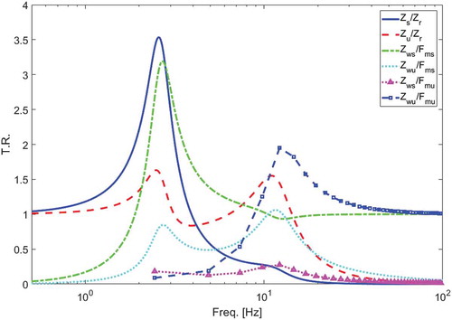
Since the basic dynamic system is the same, the system dynamics as represented by the denominator expression D is the same throughout; hence, any differences in the transmissibility ratios are due to the numerator expressions. Figure 2 shows the transmissibility ratios plotted over frequencies from zero to 35 Hz, which covers a typical range for vehicle ride dynamic frequencies (Cebon, 1999; Gillespie, 1992; Rao et al., 2008). In the following two sections, the results as displayed by Figure 2 are discussed.

Figure 2. Transmissibility ratios with legends shortened for convenience, their correct representations are in Equations (11)(11) $\left({\omega }^2{Z}_s\right)/\left(M_s^{-1}{F}_s\right)=D^{-1}\left\{{\omega }^2{M}_s\left[K_s+K_t-{\omega }^2{M}_u+j\omega \left(C_s+C_t\right)\right]\right\}$(11) –(14(14) $\left({\omega }^2{Z}_u\right)/\left(M_u^{-1}{F}_u\right)=D^{-1}\left[{\omega }^2{M}_u\left(K_s-{\omega }^2{M}_s+j\omega C_s\right)\right]$(14) )

4.1. Estimation of road profiles $z_r$ through sprung mass and unsprung mass accelerations

The graphs for $Z_s/Z_r$ and $Z_u/Z_r$ in Figure 2 show the transmissibility ratios of sprung mass and unsprung mass displacements to road profiles plotted over spatial frequencies. Both ratios are at unity for very low spatial frequencies from 0.01 to 0.1 cycles m⁻¹. As expected, the ratio $Z_s/Z_r$ is more amplified around sprung mass resonance than the ratio $Z_u/Z_r$ and vice versa around the unsprung mass resonance. This may imply that a road profile reconstruction model is more likely to behave in an unstable manner over the sprung resonance when one uses sprung mass responses than when unsprung mass responses are used, and the converse is also true. In effect, both sprung mass and unsprung mass responses can be used for reconstruction of the road profiles with a conscious effort to avoid excitation of both sprung mass and unsprung mass resonances. The ratio $Z_s/Z_r$ is severely attenuated after sprung mass resonance such that for higher frequencies, the reconstructed profile may require high levels of amplification. This implies that estimation of higher frequency content in the reconstructed profiles will be poor when only sprung mass accelerations are used. On the other hand, unsprung mass responses may be used for estimation of higher frequency content with minimal signal amplification demands as depicted by the trend of the $Z_u/Z_r$ graph in Figure 2. However, mounting a transducer over the vehicle axle may provide some practical challenges, especially for smartphone-based measurements. Therefore, sprung mass responses are used with the host vehicle being driven at much slower speeds while avoiding excitation of the sprung mass resonance.

4.2. Estimation of body forces $f_s$ and axle forces $f_u$ through sprung mass and unsprung mass accelerations

The estimation of body forces $F_s$ using accelerations from the sprung mass can be accurate at frequencies above the sprung mass resonance. Figure 2 shows that the ratio $Z_{ws}/F_{ms}=\left({\omega }^2{Z}_s\right)/\left(M_s^{-1}{F}_s\right)$ is very small for frequencies lower than the sprung mass resonance and almost remain constant at unity for higher frequencies. At the higher frequencies, the forces are transmitted without loss and the transmissibility ratio does not vary with changes in suspension stiffness. However, this also implies that it might be difficult to distinguish among different input body forces if the excitation frequencies are not properly analysed or known a priori.

On the other hand, the ratio $Z_{wu}/F_{ms}=\left({\omega }^2{Z}_u\right)/\left(M_s^{-1}{F}_s\right)$ exhibits a dynamic behaviour very similar to that of the transmissibility of the road input with respect to unsprung mass responses, with the only significant differences occurring at much lower frequencies below the sprung mass resonance. This implies that it may be hard to distinguish between the effects on the unsprung mass responses by road inputs, and forces applied directly to the sprung mass for higher frequencies. However, from the figure, it is theoretically possible to distinguish the effects by conducting low-frequency testing to determine the road inputs and then later subtract the effects of these road inputs from the overall effects.

From the foregoing discussion, it may be more preferable to use sprung mass accelerations than unsprung mass accelerations for reconstruction of sprung mass forces. It should, however, be noted that this is true when the vehicle is excited at frequencies above wheel hop resonance. For estimation of axle forces $f_u$, almost a similar situation is displayed by Figure 2 in which the transmissibility $Z_{wu}/F_{mu}$ remain at unity at frequencies higher than wheel hop resonance while the transmissibility ratio $Z_{ws}/F_{mu}$ is highly diminished (below 0.3) at all frequencies. For higher suspension stiffness, this ratio increases around the sprung mass resonance; however, it does not significantly affect the other frequencies. Therefore, reconstruction of forces applied directly to the unsprung mass can only be achieved by response measurements on the unsprung mass itself. A similar observation in Figure 2 to the possibility of isolating the effects of road inputs from the effects of the axle forces may also be made at the unsprung mass responses.

5. Results and discussions

In this section the performance of the methodology is presented through evaluations on numerical case study in Section 5.1 and experimental case study in Section 5.2. In the numerical case study, the performance was examined under changing vehicle speeds, vehicle suspension properties, noise, nonlinear suspension, while the experimental case study demonstrates the performance of the methodology over a speed bump.

5.1. Numerical study

The vehicle properties used in this numerical study are tabulated in Table 1 The suspension stiffness and damping constants have been varied a lot during the numerical study but the values used in the table are the ones that have been used for most of the results that are presented in this section.

Table 1. Numerical model properties

Property	Quantity
Sprung mass, $M_s$	4450 kg
Unsprung mass, $M_u$	420 kg
Suspension stiffness constant, $K_s$	1000 kN m^−1
Suspension damping constant, $C_s$	15 kN s m^−1
Tyre stiffness constant, $K_t$	1950 kN m^−1
Tyre damping constant, $C_t$	1 kN s m^−1

5.1.1. Changing vehicle speed

The reconstruction algorithm was tested for bump and pseudo-random profiles at the following four randomly selected vehicle speeds: 15 kmh⁻¹, 40 kmh⁻¹, 80 kmh⁻¹, and 120 kmh⁻¹. Three bump profiles (half-sinusoidal, triangular and square bumps) located on the same stretch of road and spaced 25 m apart were tested. Normally distributed white noise with an RMS of 3 mm was added to the bumps in order to replicate typical background road roughness and also to offset numerical problems that result from division by zero during numerical integration. The profiles were applied to a quarter car model to calculate corresponding sprung mass and unsprung mass accelerations. Thereafter, these accelerations were applied to the procedure presented in Section 3. The results are plotted in Figure 3(a–d). The plotted results show that there is a tendency towards smoothing the shape of the bump profiles as the speeds increase. This is very conspicuous in both the triangular and square-shaped waveforms. For accurate geometry reconstruction, it is recommended to keep vehicle speeds lower. Of course, this is dependent on the width of the bump profile in the driving direction. Shorter bumps may pose problems even for slow transverse speeds. Since the proposed reconstruction procedure is based on numerical integration, it cannot perfectly reconstruct sudden changes in geometry (as with triangular and square bumps in Figure 3(a–d)) due to large gradients around those points.

Figure 3. Results of bump tests on a numerical study at vehicle speeds of: (a)15 km h⁻¹, (b) 40 km h⁻¹, (c) 80 km h⁻¹, and (d) 120 km h⁻¹

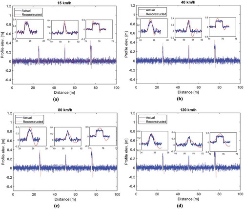
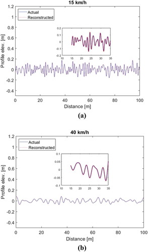
Smoothening of bump profiles at higher vehicle speeds is caused by the filtering effects of the vehicle speed which attenuate all vibrations beyond 1.5 times unsprung mass resonant frequency. Furthermore, it can be noted that noise effects are kept minimal by the inherent combined filtering effects of the mechanical system and the vehicle speed. The filtering effects of increased vehicle speeds are clearer in the reconstructed road profiles for pseudo-random surfaces shown in Figure 4(a–d). The plotted FFT for each sub-figure shows how the reconstructed profiles get more and more diminished at frequencies beyond unsprung mass resonance. The zoomed-in inserts over the road profile graphs show how smoother the profiles become with increased vehicle speed. Although this effect is evident in both the bump and random profiles, it is quite conspicuous in the random profiles especially at 120 km h⁻¹.

Figure 4. Results of random rough road tests on a numerical study at vehicle speeds of: (a) 15 km h⁻¹, (b) 40 km h⁻¹, (c) 80 km h⁻¹, and (d) 120 km h⁻¹. FFT Transmissibility ratio (____); Reconstructed (—); FFT Actual (-.-.-.)

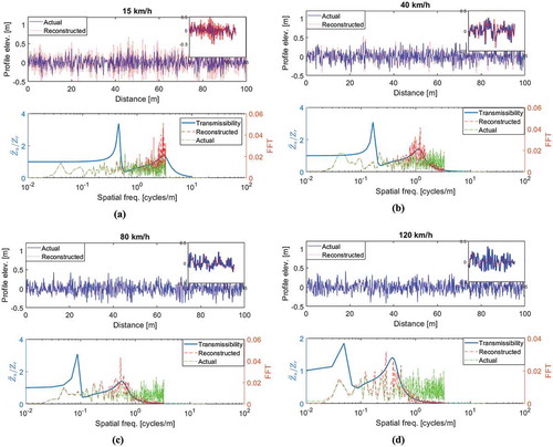
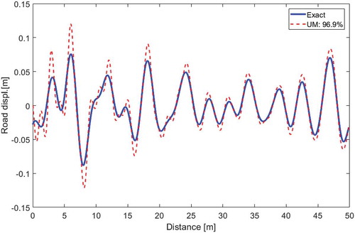
In Figure 4(a), it is noted that the FFT for the actual random profile falls within the range of the unsprung mass resonant frequency. The transmissibility ratio curve shows that at 15 km h⁻¹ the unsprung mass resonance corresponds to a spatial frequency of 3 cycles m⁻¹ while at 120 km h⁻¹ the spatial frequency is at 0.4 cycles m⁻¹. The FFT graphs further show perfect match up to around a spatial frequency of about one-third of the unsprung mass resonant frequency, after which the reconstructed profiles are increasingly amplified due to numerical instabilities around resonance and then starts to decline after resonance. Thus, if both actual and reconstructed profiles are low-pass filtered to within one-third of the unsprung mass resonance, as shown in Figure 5(a,b), it is possible to have a perfect match between the actual and reconstructed profiles. However, the problem with that is that the actual road profile progressively changes with the vehicle speed and it can be quite misleading.

Figure 5. Actual (____) and reconstructed (….) profiles low-pass filtered with a cut-off equal to one-third of unsprung mass resonance: (a) at 15 km h⁻¹, (b) at 40 km h⁻¹

5.1.2. Vehicle suspension properties

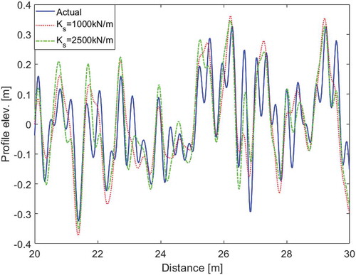
The transmissibility ratios shift towards higher spatial frequencies with an increase in the suspension stiffness (see Figure 6). However, the shift is not much and it can be expected that the range of spatial frequencies within which the technique can reproduce accurate reconstructions are similar between the two suspension stiffnesses. This may imply that minor variations in suspension stiffnesses, probably caused by degrading shocks, may not drastically affect the accuracy of the technique for the same vehicle. Note that in the example plotted in Figure 6, there is a shift of about 0.2 cycles m⁻¹ at both vehicle speeds for a suspension stiffness variation from 1000 kN m⁻¹ to 2500 kN m⁻¹. The effect of vehicle speed variation, however, is quite substantial. The transmissibility ratios are increasingly amplified at the sprung mass resonance with an increase in suspension stiffness because unsprung mass accelerations increase with increased suspension stiffness. Figure 7 shows results for a random rough profile reconstruction for these two suspension stiffnesses. The reconstructed profiles are quite close to each other, and the minor differences in the reconstructed profiles may be averaged out by any roughness classification calculation that is normally applied to roads. Therefore, there seems to be no need for calibrating the system across different suspension stiffnesses.

Figure 6. Transmissibility ratios for two different suspension stiffnesses at 20 km h⁻¹ and 120 km h⁻¹

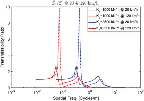
Figure 7. Effects on due to different suspension stiffnesses

5.1.3. Noise effects

In order to assess the effects of noise, different levels of noise were added to the sprung and unsprung mass accelerations. These noise polluted accelerations were then applied to the reconstruction procedure assuming combined use of sprung mass and unsprung mass accelerations. The different noise levels are presented in Table 2 as signal-noise-ratios (SNR. Table 2 shows no significant differences for SNR from 0.1 to 0.3, hence the technique can be said to be robust in the presence of noise or disturbances at SNR levels below 0.3.

Table 2. Fitting accuracies at different noise levels

SNR	Accuracy (%)
0.1	99.2
0.2	99.2
0.3	98.8
0.4	97.8
0.5	96.9

5.1.4. Nonlinear suspension forces

Damping in most vehicle suspensions cannot be accurately modelled as linear viscous dampers, due to presence of many factors that cause the suspensions to behave nonlinearly. Therefore, an attempt is made in this section to evaluate the performance of the proposed reconstruction procedure in the presence of suspension nonlinearity, especially due to a nonlinear damper. The nonlinear suspension force is modelled as a friction force governed by the LuGre model given by (Do et al., 2007)

(15) $F_L\left(v,z\right)={\sigma }_{0}z+{\sigma }_1\dot{z}+{\sigma }_{2}v$(15)

where ${\sigma }_0$ is the aggregate stiffness of the contacting surface, ${\sigma }_1$ is the damping coefficient, ${\sigma }_2$ is the viscous friction constant, $v$ is the relative velocity between the two surfaces in friction contact, and $z$ and $\dot{z}$ are the deflection and rate of deflection of the bristles at the contacting surfaces ((Do et al., 2007)).

(16) $\dot{z}=v-\frac{\left|v\right|}{G\left(v\right)}z$(16)

where the function $G\left(v\right)$ is given by (Do et al., 2007) as $G\left(v\right)=\frac{1}{{\sigma }_0}\left(F_c+\left(F_s-F_c\right)e^{-{\left(v/v_s\right)}^2}\right)$.

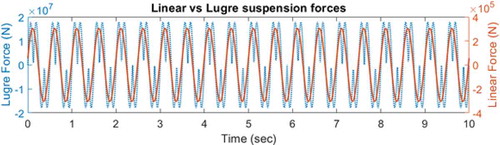
Figure 8 shows the differences in dynamic behaviour between the linear model and the LuGre model. In Figure 8 the LuGre model exhibits a discontinuity at the instance of its maximum force due to the changing friction conditions in the contact.

Figure 8. Linear vs LuGre suspension forces assuming a sinusoidal displacement input in the vehicle suspension

The result of reconstructing a random rough profile is shown in Figure 9. Despite the overshooting of the reconstructed profile, it achieves about 97% fitting accuracy. These profiles are both low-pass filtered with a cut-off of 25 Hz. Such data filtering might have contributed to a high level in fitting accuracy, by reducing the effects of the discontinuous behaviour around the turning points. This result is very encouraging considering that important vehicle frequencies fall within 25 Hz.

Figure 9. Reconstruction of a random rough profile given a nonlinear suspension damper modelled as LuGre model

5.2. Experimental study

The experimental study was aimed at verifying the performance of the developed technique on a discrete bump with known geometry and dimensions. Initially, the mechanical properties of the test vehicle were measured and translated into their corresponding quarter car model’s properties. Thereafter, a number of bump tests were conducted by driving the vehicle at a speed of approximately 20 km h⁻¹ over the same speed bump.

5.2.1. Measurement of vehicle mechanical properties

The vehicle used for the experimental study was a 2012 Toyota Fortuner with the following masses for its quarter car model: sprung mass, $M_s$ = 400 kg and unsprung mass, $M_{us}$ = 30 kg (mass of a wheel (16 kg) for a 265/65R17 tyre plus half-axle mass of (14 kg)). The vehicle has a maximum loading capacity of approximately 300 kg over the rear axle, therefore for the purposes of this study, it was tested up to a maximum load of 200 kg. In order to obtain its suspension stiffness coefficient, the vehicle was loaded and unloaded in 40 kg incrementally and decrementally up to 200 kg and back down to its unloaded state, while recording rear vehicle body and wheel deflections at each loading step. Forty kilogramme bags of building mix were used and they were loaded directly above and midway between the two rear wheels in the passengers’ cabin. The rear vehicle body deflections were recorded at two points in front and at the back of the rear wheel for both left- and right-hand rear sides of the vehicle. The final deflection was determined by averaging the four values. The suspension stiffness coefficient was approximated from deflection vs loading/unloading curves as presented in Figure 10.

Figure 10. Loading and unloading curves for the suspension measured on rear wheels

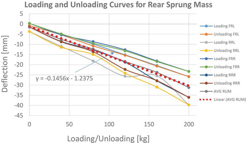
In the figure, the dotted thick graph with a deflection/load gradient of −0.1456 mm kg⁻¹ was obtained by calculating the linear regression curve for the graph representing the average deflection/load behaviour labelled as AVG RUM in the figure.

The stiffness constant for the rear axle is then calculated by inverting the deflection/load gradient and convert the resulting kg mm⁻¹ into N m⁻¹. This yields a stiffness constant of 67 376.4 N m⁻¹ for the rear axle which translates into $K_s=33687.2\mathrm{N}{\mathrm{m}}^{-1}$ on each side (in the study, $K_s\approx 33700\mathrm{N}{\mathrm{m}}^{-1}$ has been used).

The suspension damping constant was approximated by evaluating an average of the values of logarithmic decrement in graphs shown in Figure 11(a).

Figure 11. Estimation of the damping constant for the vehicle using logarithmic decrement

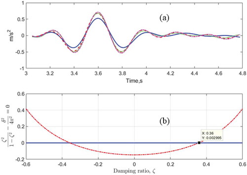
A tri-axial accelerometer in Physics Toolbox Sensor Suite Pro installed on a Samsung Galaxy Note 5 smart phone was used for measurement of vehicle accelerations. Impulsive loads (through downward jerk actions) were conducted on the vehicle rear body while the vehicle was at rest. Figure 11(a) shows z-axis accelerations measured normal to the smart phone screen. The average logarithmic decrement $\delta$ calculated from Figure 11(a) was 2.4, which is related to the damping ratio $\zeta$ by (Rao, 2011)

(17) $\delta =\frac{2\pi \zeta }{\sqrt{1-{\zeta }^2}}$(17)

The solution of equation (17)(17) $\delta =\frac{2\pi \zeta }{\sqrt{1-{\zeta }^2}}$(17) is plotted in Figure 11(b) and shows that the damping ratio, $\zeta =x\pm 0.36$. Since damping cannot be negative for the displayed behaviour of vehicle suspension, damping ratio is considered to be positive i.e. $\zeta =\mathrm{0.36.}$ The damping ratio is further related to the mass, stiffness and damping constants by the expression (Rao, 2011):

(18) $\zeta =\frac{C_s}{2\sqrt{K_s{M}_s}}$(18)

Thus, the suspension damping constant, $C_s$ can be calculated as

(19) $C_s=2\zeta \sqrt{K_s{M}_s}=2643.5\mathrm{N}\mathrm{s}/\mathrm{m}$(19)

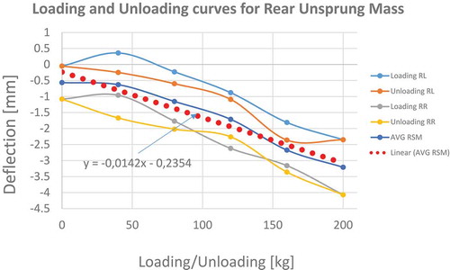
The stiffness constant of the wheel was estimated from the gradient of the linear curve shown in Figure 12, which translates to 690 845 N/m for both rear wheels. Thus, each wheel was estimated to have a stiffness constant of $K_{us}=345422.5\mathrm{N}/\mathrm{m}$ (a value of 345 400 N/m has been used in this study).

Figure 12. Loading and unloading deflection/load behaviour on the rear axle

It has been assumed that the wheels have negligible damping, but for the purposes of the reconstruction procedure proposed in this study, a value of 100 N s m⁻¹ was used. The tyres have a maximum inflation pressure of 300 kPa with recommended inflation pressure of 210 kPa on all tyres. However, inflation pressures were maintained at 200 kPa throughout the testing period.

The tests were conducted on two similar speed humps that are positioned 70 m apart along a road. Two test runs were performed and the vehicle was driven at speeds between 20 km h⁻¹ and 30 km h⁻¹ (to be exact at average speeds of 21.6 km h⁻¹ for the first test run, and 25.2 km h⁻¹ for the second test run). Both test runs were conducted while driving the vehicle in the same direction. It was extremely difficult to precisely control and measure the speed of the vehicle while traversing the hump, so that it can be expected that the real speeds over the humps are quite dissimilar.

The smartphone was firmly secured to the floor of the passenger cabin above the rear axle using several strips of sticky tape. The z-axis accelerations (positive outwards and normal to the screen) were extracted and applied to the proposed reconstruction procedure. Since these accelerations were measured on the vehicle body, only sprung mass accelerations were used in the procedure. This was a more practical approach since there was no other way of mounting the smartphone on the vehicle axle without need for adding extra fixtures to the vehicle body.

Figure 13(a,b) plots the reconstructed bumps over exact humps for the two test runs. For clarity on the accuracy of the reconstructed hump profiles, inserts of the zoomed-in graphs around the humps themselves are shown in the figure.

Figure 13. Bump profile reconstruction using acceleration measurements on a Toyota Fortuner

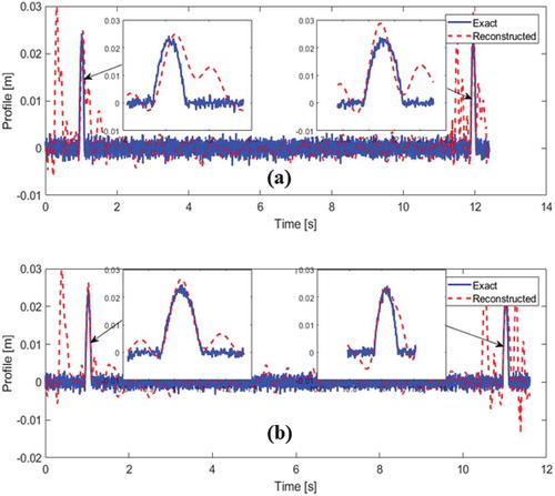
There are two very significant observations on the results: firstly, the reconstruction algorithm exhibits a hump in front of the real bump due to the effect of the front tyre when it was traversing the same bump; secondly, the reconstructed humps have sidelobes to the right side which might be caused by a combination of rear wheel harsh landing and the numerical problems of the numerical integration algorithm to perfectly reconstruct a sudden change in geometry. Apart from these two problems, the algorithm promises to provide a much easier and faster means of road profile reconstruction, taking about 32.4 s to process two sequences of 5801 data points on a Dell Precision Tower 7910 running 64-bit Windows 10 Pro, 64 GB RAM, 2.10 GHz, Intel(R) Xeon CPU E5-2620 v4. The mathematics involved in performing this procedure are quite tractable as compared to the widely used Kalman filtering method (Kang et al., 2019). The question still remains on how well it can replicate the good approximation capabilities as demonstrated by numerical studies when evaluated on random rough roads and how easily it can be applied across different vehicles with different properties. These are obvious questions for further investigation in this work.

6. Conclusions

The procedure for road profile reconstruction by reversing the forward ride problem is developed and demonstrated via a numerical and experimental study at different vehicle speeds, with different suspension stiffnesses, a nonlinear damper, and under different levels of noise. Analysis of the transmissibility ratios shows that the procedure yields accuracies with more than 97% correlation when the road profiles are filtered to within one-third of the unsprung mass resonance, which makes it automatically ideal for low-speed applications. For frequencies higher than 1.5 times the unsprung mass resonance, the procedure may require implementation of an amplifying module.

The tests for different vehicle suspension stiffnesses and in nonlinear damping conditions were conducted to evaluate the stability of the procedure. It is observed that there is no significant differences introduced by different suspension stiffnesses and the nonlinear damper. This might be due to the fact that the upper cut-off of 25 Hz inherently filtered out the higher frequency effects. There were notable overshoots for the nonlinear model around the turning points.

The profile reconstruction procedure takes shorter time, which makes it suitable for online implementation. For example, the whole process from calculation of the accelerations and profile reconstruction for two sequences of 5801 data points took under 33 s on a Dell Precision Tower 7910 running 64-bit Windows 10 Pro, with 64 GB RAM, and at a CPU 2.10 GHz.

The need for system characterisation for this procedure makes it ideal for light-weight vehicles where system parameters such as the vehicle and axle weights, suspension stiffness and damping constants, and tyre stiffness constants can be more easily determined than in heavy vehicles. Heavy vehicle applications may require the use of artificial intelligence procedures where system characterisation is not required.

Disclosure statement

No potential conflict of interest was reported by the authors.

Additional information

Funding

The research was not funded by any institution.

Notes on contributors

H.M. Ngwangwa

Dr Harry Magadhlela Ngwangwa graduated with a Bachelor of Science Mechanical Engineering degree from the University of Malawi in 1995, and worked for the same university for a number of years before obtaining a Bachelor of Science Hons: Mechanics (2003), Master of Science: Mechanics (2005), and later (2015), a Doctor of Philosophy degree at the University of Pretoria. During his masters degree research he investigated and published his findings on structural damage assessment of a cracking beam, and investigated condition monitoring of road surfaces using measured vehicle responses employing artificial neural networks modelling, for his doctoral research. He is currently working for the University of South Africa as a senior lecturer and continues to research in the area of structural condition monitoring. This study is a sequel to his doctoral degree research.

References

- Allouch, A., Koubaa, A., Abbes, T., & Ammar, A. (2017). RoadSense: Smartphone application to estimate road conditions using accelerometer and gyroscope. IEEE Sensors Journal, 17(13), 4231–20. https://doi.org/10.1109/JSEN.2017.2702739
- Becker, C. M., & Els, P. S. (2014). Profiling of rough terrain. International Journal of Vehicle Design, 64(2–4), 240–261. https://doi.org/10.1504/IJVD.2014.058500
- Bidgoli, M. A., Golroo, A., Nadjar, H. S., Rashidabad, A. G., & Ganji, M. R. (2019). Road roughness measurement using a cost-effective sensor-based monitoring. Automation in Construction, 104, 140–152. https://doi.org/10.1016/j.autcon.2019.04.007
- Cebon, D. (1999). Handbook of vehicle-road interaction. Swets & Zeitlinger Publishers.
- Celaya-Padilla, J. M., Galván-Tejada, C. E., López-Monteagudo, F. E., Alonso-González, O., Moreno-Báez, A., Martinez-Torteya, A., Galván-Tejada, J., Arceo-Olague, A., Luna-Garcia, H., & Gamboa-Rosales, H. (2018). Speed bump detection using accelerometric features: A genetic algorithm approach. Sensors, 18(2), 443. https://doi.org/10.3390/s18020443
- Directorate for Science, Technology and Industry (DSTI). (1998). Scientific expert group IR6 on the dynamic interaction between vehicles and infrastructure experiment (DIVINE Project): Technical report (DSTI/DOT/RTR/IR6(98)1/FINAL (unclassified)). OECD.
- Do, N. B., Ferri, A. A., & Bauchau, O. A. (2007). Efficient simulation of a dynamic system with LuGre friction. Journal of Computational and Nonlinear Dynamics, 2(4), 281–289. https://doi.org/10.1115/1.2754304
- Fox, A., Kumar, B. V. K. V., Chen, J., & Bai, F. (2017). Multi-lane pothole detection from crowdsourced undersampled vehicle sensor data. IEEE Transactions on Mobile Computing, 16(12), 3417–3430. https://doi.org/10.1109/TMC.2017.2690995
- Gillespie, T. D. (1992). Fundamentals of vehicle dynamics. SAE International.
- Gonzalez, A., O’Brien, E. J., Li, Y. Y., & Cashell, K. (2008). The use of vehicle acceleration measurements to estimate road roughness. Vehicle System Dynamics, 46(6), 485–501. https://doi.org/10.1080/00423110701485050
- Harikrishnan, P. M., & Gopi, V. P. (2017). Vehicle vibration signal processing for road surface monitoring. IEEE Sensors Journal, 17(16), 5192–5197. https://doi.org/10.1109/JSEN.2017.2719865
- Hugo, D., Heyns, P. S., Thompson, R. J., & Visser, A. T. (2008). Haul road defect identification using measured truck response. Journal of Terramechanics, 45(3), 79–88. https://doi.org/10.1016/j.jterra.2008.07.005
- Hull, B., Bychkovsky, V., Zhang, Y., Chen, K., Goraczko, M., Miu, A., Shih, E., Balakrishnan, H., & Madden, S. (2006) Car Tel: A distributed mobile sensor computing system. Proceedings of the 4th ACM on Embedded Networked Sensor Systems, Oct 31-Nov 3.
- Kang, S.-W., Kim, J.-S., & Kim, G.-W. (2019). Road roughness estimation based on discrete Kalman filter with unknown input. Vehicle System Dynamics, 57(10), 1530–1544.
- Kropac, O., & Mucka, P. (2008). Indicators of longitudinal unevenness of roads in the USA. International Journal of Vehicle Design, 46(4), 393–415. https://doi.org/10.1504/IJVD.2008.020306
- Mohan, P., Padmanabhan, V. N., & Ramjee, R. (2008). Nericell: Rich monitoring of road and traffic conditions using mobile smartphones. Proceedings of the 6th ACM on Embedded Networked Sensor Systems, Nov 5–7.
- Ngwangwa, H. M., Heyns, P. S., Breytenbach, A., & Els, P. S. (2014). Reconstruction of road defects and road roughness classification using artificial neural networks simulation and vehicle dynamic responses: Application to experimental data. Journal of Terramechanics, 53, 1–18. https://doi.org/10.1016/j.jterra.2014.03.002
- Ngwangwa, H. M., Heyns, P. S., Labuschagne, F. J., & Kululanga, G. K. (2010). Reconstruction of road defects and road roughness classification using vertical vehicle accelerations with artificial neural networks simulation. Journal of Terramechanics, 47(2), 97–111. https://doi.org/10.1016/j.jterra.2009.08.007
- Paterson, W. D. O. (1987). Road deterioration and maintenance effects: Models for planning and management. A World Bank Publication: The Highway Design and Maintenance Series. The Johns Hopkins University Press.
- Pesterev, A. V., Bergman, L. A., & Tan, C. A. (2004). A novel approach to the calculation of pothole-induced contact forces in MDOF vehicle models. Journal of Sound and Vibration, 275(1–2), 127–149. https://doi.org/10.1016/S0022–460X(03)00789-2
- Pesterev, A. V., Bergman, L. A., Tan, C. A., & Yang, B. (2005). Application of the pothole DAF method to vehicles traversing periodic roadway irregularities. Journal of Sound and Vibration, 279(3–5), 843–855. https://doi.org/10.1016/j.jsv.2003.11.061
- Rahman, S. A., Mourad, A., Barachi, M. E., & Orabi, W. A. (2018). A novel on-demand vehicular sensing framework for traffic condition monitoring. Vehicular Communications, 12, 165–178. https://doi.org/10.1016/j.vehcom.2018.03.001
- Rao, D. V., Jian, P., Mohamad, Q. S., Gang, S., & Zuo, S. (2008). Road vehicle dynamics. SAE International.
- Rao, S. S. (2011). Mechanical vibrations. Prentice Hall.
- Roadroid. (2019, December). Road surveys using smartphone; s [Internet]. Essential guide for roadroid 2; roadroid. http://www.roadroid.com/common/References/Roadroid%20User%20Guide%20-%20Version%202%20Pro.pdf
- ROMDAS system [Internet]. (2018). Data Collection Ltd. https://romdas.com/romdas-system.html
- Sayers, M. W., Gillespie, T. D., & Paterson, W. D. O. (1986). Guidelines for conducting and calibrating road roughness measurements (A World Bank Publication: Technical Paper Number 46). The Johns Hopkins University Press.
- Sayers, M. W., & Karamihas, S. M. (1998). The little book of profiling: Basic information about measuring and interpreting road profiles. University of Michigan.
- Schnebele, E., Tanyu, B. F., Cervone, G., & Waters, N. (2015). Review of remote sensing methodologies for pavement management and assessment. European Transport Research Review, 7(2), 7. https://doi.org/10.1007/s12544-015-0156-6
- Takahashi, J., Kobana, Y., Isoyama, N., Tobe, Y., & Lopez, G. (2018). YKOB: Participatory sensing based road condition monitoring using smartphones worn by cyclist. Electronics and Communications in Japan, 101(4), 3–14. https://onlinelibrary.wiley.com/doi/abs/10.1002/ecj.12027
- Value of asset preservation [Internet]. South African National Roads Agency Ltd (SANRAL). https://www.nra.co.za/live/content.php?Item_ID=185
- Xue, G., Zhu, H., Hu, Z., Yu, J., Zhu, Y., & Luo, Y. (2017). Pothole in the dark: Perceiving pothole profiles with participatory urban vehicles. IEEE Transactions on Mobile Computing, 16(5), 1408–1419. https://doi.org/10.1109/TMC.2016.2597839
- Yousefzadeh, M., Azadi, S., & Soltani, A. (2010). Road profile estimation using neural network algorithm. Journal of Mechanical Science and Technology, 24(3), 743–754. https://doi.org/10.1007/s12206-010-0113-1