A new approach for ocular artifact removal from EEG signal using EEMD and SCICA

Abstract

EEG data obtained from the scalp using the electrodes, usually gets contaminated by various artifacts like muscle artifact, line interference artifact, ocular artifact, and others. The Ocular artifact which is caused due to eye-blink or other eye movements, while measuring EEG is the most common and most critical EEG artifact. For a long time, it has been a research challenge for any method to remove the ocular artifact from EEG without causing loss of the EEG signal. In this paper, a new approach is introduced to remove the ocular artifact from EEG signal using Ensemble Empirical Mode Decomposition (EEMD) and Spatial Constraint Independent Component Analysis (SCICA) without causing loss to EEG signal. The contribution of the method lies in the fact that it combines the advantages of both EEMD and SCICA. Here, EEMD is applied to the artifactual EEG signal to obtain Implicit Mode Functions (IMFs). The artifactual IMFs are separated from artifact-free IMFs by using the Correlation Coefficient-based algorithm. Now, the artifactual IMFs are provided as the input channels to Independent Component Analysis (ICA) and to obtain Independent Components (ICs) and inverse mixing matrix. Then, the Kurtosis and mMSE techniques are used to define the threshold levels for differentiating between artifactual and artifact-free ICs. Moreover, the mixing matrix is also modified using spatial constraints. The modified mixing matrix and ICs are then used to obtain restored IMFs. Finally, the artifact-free EEG signal is reconstructed by summing up artifact-free IMFs and restored IMFs. The proposed method is compared with other state-of-the-art methods in terms of Mutual Information, Correlation Coefficient, and Coherence. The results show that the proposed method has better performance as compared to other state-of-the-art methods for ocular artifact removal from EEG.

KEYWORDS:

• electroencephalogram
• independent component analysis
• independent components
• electrooculogram artifact
• spatially constrained
• ensemble empirical mode decomposition

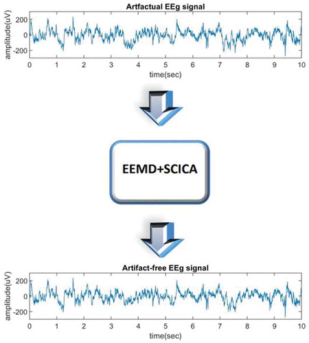
PUBLIC INTEREST STATEMENT

EEG signal is the signal obtained by placing electrodes on the scalp of a person. This signal is affected by many noises called artifacts like external and internal artifacts. The internal artifacts are related to the patients like interference from ECG signal, eye-blink, muscle, etc. In this paper, an attempt is made to remove the artifactual EEG signal affected due to ocular artifact, i.e., artifact caused by eye rotation or eye-blink. Since it is not possible to keep eyes open throughout EEG especially for children so these artifacts are very common. So, instead of discarding the artifactual signal one can de-noise it using the method given in the paper. The method utilizes the benefits of EEMD and SCICA and denoises the signal to obtain an artifactual-free signal.

1. Introduction

Electroencephalography (EEG) is the process of measurement of the electrical activities of the brain obtained by placing electrodes over the scalp of the patient. EEG helps in analyzing and investigating the human brain, also to find out brain disorders (http://emedicine.medscaple.com/article/1142008-overview). The EEG artifacts can be divided into classes of patient-related (physiological) artifacts and system artifacts. Common patient-related or internal artifacts are Electro-Myogram (EMG), ECG or pulsation, Electro-Oculogram (EOG) or Ocular artifact, ballistocardiogram, and sweating. The system or external artifacts are 50/60 Hz power supply interference, impedance fluctuation, cable defects, electrical noise from the electronic components, and unbalanced impedance of the electrodes. The ocular artifact is the most common and most critical artifact in EEG. The main cause of EOG artifacts is eye movement and eye blinks during EEG recording. A significant potential difference occurs between the cornea and the retina due to the blinking of the eye which affects the EEG recording (Hesse & James, 2005). The effect of the ocular artifact is more to the low-frequency region (up to 16 Hz) of EEG and its amplitude may reach up to 800 µV (Hagemann & Naumann, 2001). Ocular artifact creates inaccuracy in EEG measurement and can even change the EEG signal waveform entirely. Independent Component Analysis (ICA) is one of the most recently used techniques for ocular artifact removal from EEG signal (Jung et al., 1998, Makeig et al., 1996). ICA is a statistical tool, used to decompose a mixed-signal (of different recording channels) into independent components (ICs), corresponding to different independent sources (Joyce et al., 2004, Jiang et al., 2019).

To apply ICA on EEG signals some assumptions are made like (i) the sources have non-Gaussian distribution and they are mutually statistically independent and (ii) the number of recording channels must be greater or equal to the number of independent sources (or ICs). The efficiency of ICA for artifact removal from the EEG signal depends on these assumptions. So, more the number of observed signals better will be the results obtained by ICA. For this purpose, Empirical Mode Decomposition (EMD) is used with ICA (Zeng et al., 2016). By applying EMD, the signal is decomposed into various IMFs (Implicit Mode Functions) which are obtained in descending order of frequency components of the signal. These large number of IMFs and then used as input signals of ICA to obtain various ICs. So, EMD-ICA has better results as compared to zeroing-ICA. Performance of EMD is affected by problems like mode mixing and aliasing for example, mode mixing occurs when either single IMF contains different scale signals or the same scale signal is present in different IMFs (Zhaohua & Huang, 2005). This problem is tackled by using a modified version of EMD (Pramudita et al., 2017, Jiang et al., 2019) that is Ensemble Empirical Mode Decomposition (EEMD). EEMD with ICA outperforms EMD with ICA for ocular artifact removal from the EEG signal. The Performance of ICA can further be improved by applying Spatial Constraints with the mixing matrix of ICA. Spatial Constraints Independent Component Analysis (SCICA), which is a modified version of ICA, is a better choice for ocular artifact removal from EEG signal than using traditional ICA technique. In SCICA prior knowledge about the signal is incorporated for computing ICs. Moreover, SCICA also overcomes the permutation problem of ICA, though not fully but at least for constraint columns (James & Hesse, 2006, Ille, 2001). In this research work, a new approach, using a cascaded combination of EEMD and SCICA is proposed to remove the ocular artifact from the EEG signal. The method proposed has the following advantages as compared to other latest methods:

i.The efficiency of ICA is improved by using IMFs as source signals

ii.Limitations of EMD are overcome by using EEMD

iii.The efficiency of cascade combination of EEMD and ICA is improved by modifying the mixing matrix with spatial constraints i.e. by using SCICA with EEMD.

The remaining paper consists of following sections, section-2 in which the background theory is discussed, section-3 in which explanation of the proposed method is described, section-4 which includes observations and the results and finally section-5 which concludes the paper.

2. Background

The proposed method is based on EEMD algorithm, SCICA, and artifact detection parameters like kurtosis and modified Mean Sample Entropy (mMSE). So, in this section background theory and the implementation of these algorithms are discussed as subsections. In subsection 2.1 the EMD is described and its implementation is enumerated and its modification to EEMD is also stated. In subsection 2.2, SCICA is discussed in detail with its implementation. Finally, in subsection 2.3 the thresholding techniques used in the proposed method like kurtosis and modified Mean Sample Entropy (mMSE) are elaborated.

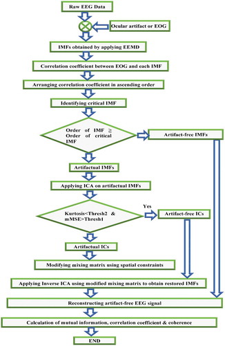
Figure 1. Block diagram of the method proposed

2.1. Ensemble empirical mode decomposition (EEMD)

EMD is the method, which is best suited for decomposing non-stationary, non-linear, and random processes like EEG signal into various IMFs (Jiang et al., 2019). An IMF represents an oscillatory mode of the signal. First IMF corresponding to highest frequency component of signal and the last IMF with lowest frequency component. Two conditions should be fulfilled by IMFs; (i) The number of extrema and zero crossings must differ at most by one (ii) The mean value of envelope defined by the local maxima and local minima is zero or one can say that they should be symmetric with respect to zero.

In case of EMD, IMFs of a signal are obtained by an iterative process known as sifting. Steps involved in sifting process are discussed in detail below (Huang et al., 1998) as

1)Extrema Identification: Find all the extrema i.e. identify all maxima and minima of signal.

2)Interpolate: Interpolate between maxima to get $x_{max}\left(n\right)$ and interpolate between minima to get $x_{min}\left(n\right)$.

3)Average Envelope: Calculate average between the envelopes, $x_{av}\left(n\right)=\left(x_{max}\left(n\right)+x_{max}\left(n\right)\right)/2$.

4)IMF Extraction: Now, subtract $x_{av}\left(n\right)$ from the original signal to obtain detail, $d_1\left(n\right)=x\left(n\right)-x_{av}\left(n\right)$and residue $r_1\left(n\right)=x\left(n\right)-d_1\left(n\right)$. Now $c_1\left(n\right)=d_1\left(n\right)$. Here $c_1\left(n\right)$is the 1^st IMF which contains the highest frequency component of the signal.

5)Stopping Criteria: Now the residue signal $r_1\left(n\right)$ is given as input to next iteration and all these steps are repeated to obtain details, residues and IMFs. These iterations are repeated until extracting all the IMFs. This sifting procedure is terminated (Huang et al., 1998, Rilling et al., 2003) when the $k^{Th}$residue $r_k\left(n\right)$becomes less than a predetermined small number or becomes monotonic. This is ensured by limiting SD (0.2–0.3) between $k^{Th}$ and ${\left(k-1\right)}^{Th}$ iterations.

6)Reconstruction: If $N$ rounds of sifting process is performed on the given signal x(t), it will be decomposed into a set of $N$ IMFs. Original signal can be reconstructed as sum of $N$ IMFs and $r_N\left(n\right)$ as given below

(1) $x\left(n\right)=\sum _{k=1}^N{c}_k\left(n\right)+r_N\left(n\right)$(1)

where $r_N\left(n\right)$ is residue after $N$ iterations.

EMD performed well but it suffers with problems of mode mixing, oscillations, and aliasing. The mode mixing and aliasing problems of EMD can be overcome by using modified version of EMD, known as EEMD (Pramudita et al., 2017). In EEMD white noises of different amplitudes are added in the original signal to obtain different IMFs. The resultant IMF is the average of various IMFs obtained by adding white noise. Different steps of EEMD algorithm are

1)White Gaussian noise $w^i\left(n\right)$($i$ =1, … …, L) is added to the original signal $x\left(n\right)$ as$x^i\left(n\right)=x\left(n\right)+\epsilon w^i\left(n\right).$where $\epsilon$ is weight coefficient of added noise.

2)Now for every $x^i\left(n\right),$ $k$ IMFs ($IM{F}_k^i\left(n\right)$) are obtained by applying EMD algorithm on $x^i\left(n\right)$. where $k=1,2,3,\dots \dots .$

3)Finally, $k^{Th}$IMF for EEMD is calculated as:

(2) $IM{F}_k\left(n\right)=\frac{1}{L}\sum _{i=1}^{L}IM{F}_k^i\left(n\right)$(2)

2.2. Spatially constraints independent component analysis (SCICA)

ICA is used to decompose mixed observed signals into Independent Components (ICs) or actual sources. The observed sources are weighted sum of ICs. For efficient decomposition using ICA, number of the observed signals should greater than or equal to actual sources. For an array of channels, which provides N observed signals

(3) $p\left(k\right)=\left[p_1\left(k\right),p_2\left(k\right),p_3\left(k\right),\dots \dots \dots ..,p_N\left(k\right)\right]$(3)

ICA decomposes it into $M\left(\mathrm{N}\ge \mathrm{M}\right)$sources/ICs as

(4) $r\left(k\right)=\left[r_1\left(k\right),r_2\left(k\right),r_3\left(k\right),\dots \dots \dots ..,r_M\left(k\right)\right]$(4)

(5) $r\left(k\right)=W\ast p\left(k\right)$(5)

where, $W$ is the inverse mixing matrix which is defined in such a way that the mutual information is minimized among all ICs in the decomposition process.

ICA is mainly used to obtain the value of unmixing matrix $W$, ICs and mixing matrix $A$. SCICA is modified version of ICA (James & Hesse, 2006). In this case, the mixing matrix$A$ is modified by applying Spatial Constraints to the columns of mixing matrix using prior knowledge about signal. The modified mixing matrix,$\text{^}A$ consists of two parts as $\text{^}A$ = [$\text{^}{A}_C{A}_U$], where $\text{^}{A}_C$is the spatially constrained columns and $A_U$ are unconstrained columns. The spatially constrained columns are obtained either by using hard constraints or soft constraints. For applying hard constraints, $\text{^}{A}_C$= $A_C$ is considered, where $A_C$ represents the predefined constraint sensor projections treated as reference, which are in accordance with the constraints considered in (Ille, 2001). Though it is simple to apply the hard constraints but it limits the accuracy of SCICA so soft constraints are preferred over hard constraints (Hesse & James, 2005). The soft constraints limit the divergence between the constrained column $\text{^}{A}_C$ and their corresponding reference topographies $A_C$ by a threshold value $\alpha$. Consider $a_c$ and $\text{^}{a}_c$, where $a_c$ and $\text{^}{a}_c$ represents unit norm column vector correspond to associate columns of $A_C$ and $\text{^}{A}_C$, respectively.

The main process to implement soft constraints, is to ensure that $\text{^}{a}_c$ and $a_c$ subtend an absolute angle not greater than angular threshold $\alpha$ (0 <$\alpha <\pi /2$) (Hesse & James, 2005). It can be explained in following steps (Hesse & James, 2005): -

1)If $\left|a\mathrm{c}\mathrm{o}\mathrm{s}\left(a_c^T\text{^}{a}_c\right)\right|$< α then $\text{^}{a}_c$is not changed.

2)Otherwise $\text{^}{a}_c$ is projected towards $a_c$ to make $\left|a\mathrm{c}\mathrm{o}\mathrm{s}\left(a_c^T\text{^}{a}_c\right)\right|$ = α. This projection involves forming a new unit norm vector $y=p{a}_c+\left(1-p\right)\text{^}{a}_c$ with $0\le p\le 1$ and cos(α) = $\left|{\hat{a}}_c^T\right|/∥y∥$

3)The value of $p$ is given by square root of quadratic equation $c_1{p}^2+c_{2}p+c_3$= 0.

where,

(6) $c_1=1+2a_c^T\text{^}{a}_c+(a_c^T\text{^}{a}_c{)}^2-((2-2a_c^T\text{^}{a}_c)co{s}^2\left(\alpha \right))$(6)

(7) $c_2=(2a_c^T\text{^}{a}_c+2(a_c^T\text{^}{a}_c{)}^2)-((2a_c^T\text{^}{a}_c-2)co{s}^2\left(\alpha \right))$(7)

(8) $c_3=(a_c^T\text{^}{a}_c{)}^2-co{s}^2\left(\alpha \right)$(8)

This value of p is substituted into the expression for y and value of $\text{^}{a}_c$ is calculated as $\text{^}{a}_c$=$\frac{y}{∥y∥}$.

2.3. Modified mean sample entropy(mMSE) and Kurtosis

Entropy is mainly used to detect randomness in a signal. According to Bos et al. (Bosl et al., 2011) modified Mean Sample Entropy (mMSE) gives more information about regularities of EEG time series in comparison to Single-Scale Entropy. For a mono-variate discrete signal $X=\left\{x_1,x_2,\dots \dots \dots .\dots x_N\right\}$, mMSE is calculated (Mahajan & Morshed, 2015) as

(9) $mMSE\left(m,r\right)=log\left(\frac{{B_r}^m}{{A_r}^m}\right)$(9)

where $m$ is the length of patterns that are compared to each other and $r$ is tolerance, $B_r$ and $A_r$ are the counters to track $m$ and $\left(m+1\right)$ template match within the tolerance value $r$ respectively. In terms of template vector pairs, $A_r$ is the number of template vector pairs (of length $m+1$) having distance $d\left\{X_{m+1}\left(i\right),X_{m+1}\left(j\right)\right\}<r$ and $B_r$ is the number of template vector pairs (of length $m)$ having distance $d\left\{X_m\left(i\right),X_m\left(j\right)\right\}<r$.

As per (Mahajan & Morshed, 2015) and other, $m=2$ and $r$ = 2 $\times$ Standard deviation of the data sequence of IC.

Kurtosis (Mahajan & Morshed, 2015) is a fourth-order statistical parameter, which is used to study the peaked-ness of distribution of any random variable and is calculated as

(10) $K=m_4-3m_2^2$(10)

and

(11) $m_n=E\left\{{\left(x-m_1\right)}^2\right\}{m}_4$(11)

where, $m_n$, $m_1$ and $E$ are $n^{th}$ order moment, mean and expectation function of random variable $x$.

3. Proposed method

The proposed method has following five major steps:

I.Decomposition of artifactual EEG signal into IMFs using EEMD.

II.Classification of IMFs as artifactual IMFs and artifact-free IMFs.

III.Decomposition of Artifactual IMFs into ICs using ICA and classification of ICs based on values of kurtosis and mMSE.

IV.IMF restoration by applying Spatial Constraints in mixing matrix and reconstruction of the artifact-free EEG signal

V.Performance analysis of proposed method in terms of Mutual Information, Correlation Coefficient, and Coherence.

The algorithm needs to be performed in the above-mentioned order. As we know, the performance of ICA improves if the number of inputs is increased, this is ensured by applying EEMD prior to ICA. Spatial constraints can only be applied once the mixing matrix is obtained by applying ICA so it follows ICA. Finally, the performance analyzing parameters are calculated to compare results with state-of-the-art methods.

The above steps are depicted in block diagram shown in Figure 1.

3.1. Decomposition of the artifactual EEG signal into IMFs using EEMD

Before performing decomposition, the artifactual signal is obtained using the real time EEG signal. The real time EEG signal with no ocular artifact is obtained from physio.net. Then, ocular artifact is modeled in the MATLAB with the amplitude and frequency as mentioned in the introduction section. Finally, the artifactual EEG signal is obtained by adding ocular artifact to the real time EEG signal. This artifactual EEG is then decomposed into true IMFs by using EEMD algorithm.

3.2. Classification of IMFs in two classes of artifactual IMFs and artifact-free IMFs

In this step, IMFs are classified as artifactual IMFs and artifact-free IMFs. Correlation Coefficient between each IMF and EOG artifact is calculated. These Correlation Coefficients are arranged in ascending order and absolute value of difference between adjacent Correlation Coefficient is calculated. The critical IMF is identified as the IMF for which this absolute value of difference between adjacent Correlation Coefficient is maximum (Wang et al., 2016). As it is known that lower order IMFs have high-frequency components and higher order IMFs have lower frequency components (Rilling et al., 2003) and EOG affects only lower frequency components (0–16 Hz) of EEG signal (Hagemann & Naumann, 2001) so, all the IMFs above this critical IMF are considered to be artifactual in nature.

3.3 Decomposition of artifactual IMFs into ICs using ICA and classification of ICs based on values of kurtosis and mMSE

In this step, artifactual IMFs are decomposed into ICs using ICA and then classified into two classes based on the values of mMSE and kurtosis. The artifactual IMFs are used as the input signals to ICA and various ICs are obtained. Many algorithms are designed to perform ICA. For sources having super-Gaussian distribution, infomax ICA (Makeig et al., 1996) is the most efficient algorithm. The approximate model for real-time EEG with the ocular artifact is closest to super-Gaussian distribution so, in the proposed method, infomax ICA is selected among different ICA algorithms.

The values of mMSE and kurtosis are calculated for each IC using formulas (9), (10) and (11). The value of mMSE for ocular artifactual EEG signal is low as its pattern is more predictable as compared to the pattern of artifact-free EEG signal (Mahajan & Morshed, 2015). The signals with peak distribution have higher values of kurtosis so the value of kurtosis for ocular artifact affected signal will be higher as compared to its values for real-time EEG signal (Mahajan & Morshed, 2015).

In the proposed method, the number of the ICs is less so two-sided t-distribution (with 95% CI) is preferred and threshold values for mMSE and Kurtosis are calculated by using two-sided 95% Confidence Interval (CI) of the mean for t-distribution. The threshold value for mMSE (lower limit of 95% CI of the mean) (Mahajan & Morshed, 2015) is calculated as

(12) $Lowerlimit\left(Thresh1\right)=\bar{x}-\frac{s}{\sqrt{N}}\ast t_{N-1}$(12)

The threshold value for Kurtosis (upper bound of the 95% CI of the mean) (Mahajan & Morshed, 2015) is calculated as

(13) $Upperlimit\left(Thresh2\right)=\bar{x}+\frac{s}{\sqrt{N}}\ast t_{N-1}$(13)

where, $\bar{x},s$, and $N$ are samples mean, standard deviation and number of ICs, respectively. For the two-tailed test with 95% significance level, $t_{N-1}=2.201$(Mahajan & Morshed, 2015).

Now kurtosis and mMSE values of each IC are compared with threshold values of mMSE kurtosis and. If mMSE < Thresh1 or kurtosis > Thresh2 then IC is classified as artifactual IC otherwise it is classified as artifact-free IC.

3.4 IMF restoration by applying spatial constraints in mixing matrix and reconstruction of the artifact-free EEG signal

When the artifactual IMFs are used as the input signals of ICA to obtain various ICs, n^th column of mixing matrix is corresponding to n^th IC. This mixing matrix is modified by applying Spatial Constraints to the columns of mixing matrix corresponding to artifactual ICs. Restored IMFs are obtained by using artifactual ICs, artifact-free ICs and modified mixing matrix. Finally, artifact-free EEG signal is reconstructed by summing up restored IMFs and artifactual IMFs.

3.5 Performance analysis of proposed method in terms of mutual information, correlation coefficient and coherence

Proposed method is compared with other latest methods in terms of Mutual Information, Correlation Coefficient and Coherence of artifact-free EEG signal. Mutual Information (MI) is defined as the quantity which measures amount of information one random variable gives about another random variable. MI can be calculated by Kullback–Leibler distance between the product of the marginal pdfs of random variables $a$ and $b$ and their joint pdf, which can be given as(Mahajan & Morshed, 2015)

(14) $MI\left(a,b\right)=\int \underset{-\mathrm{\infty }}{\overset{\mathrm{\infty }}{\int }}f\left(a,b\right)\mathrm{l}\mathrm{o}\mathrm{g}\left(\frac{f\left(a,b\right)}{f\left(a\right)f\left(b\right)}\right)dadb$(14)

where $f\left(a\right)$ and $f\left(b\right)$ are individual marginal pdfs and $f\left(a,b\right)$ is the joint pdf. Here $a,b$ are real-time EEG signal and artifact-free EEG signal, respectively. Mutual information is large if two random variables are closely related.

Correlation Coefficient is used to measure linear relationship between two random variables. It uses second order statistics to measure similarity between random variables. It is mathematically given by (Mahajan & Morshed, 2015).

(15) $r_{ab}=\frac{cov\left(a,b\right)}{{\sigma }_a{\sigma }_b}$(15)

where $cov$ is covariance and σ is the standard deviation.

Coherence measures the degree of linear dependency of two signals by testing for similar frequency components. It is used to analyze performance in the frequency domain. It is calculated in magnitude square term (Mahajan & Morshed, 2015) as

(16) $C_{ab}\left(f\right)=\frac{{\left|G_{ab}\left(f\right)\right|}^2}{G_{aa}\left(f\right)G_{bb}\left(f\right)}$(16)

where $G_{ab}\left(f\right)$ is cross spectral density, $G_{aa}\left(f\right)$ is the auto spectral density of random variable $a$ and $G_{bb}\left(f\right)$ is the auto spectral density of random variable $b$.

4. Results

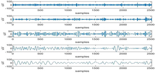
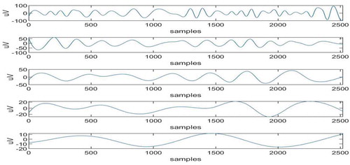
The proposed method is verified for real-time EEG data, obtained from physionet.org (www.physionet.org sampling frequency and duration of 10 sec. The ocular artifact is added to the real-time signal between 3^rd and 4^th sec and also between 7^th and 8^th sec. The real-time signal and artifactual EEG signal are shown in Figure 2. By focusing on both the signal graphs in the time instants between 3^rd and 4^th sec and also between 7^th and 8^th sec one can observe that ocular artifact is added to the second signal. The proposed algorithm will be applied on artifactual signal that is second signal in the graph to remove the ocular artifact. Now, EEMD is applied to the artifactual EEG signal and 10 IMFs are obtained first 5 are shown in Figure 3, and next 5 are shown in Figure 4. It can be clearly seen from these figures that IMFs are obtained in decreasing order of the frequency components.

Figure 2. Real-time EEG signal and artifactual EEG signal

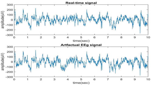
Figure 3. IMFs (1 to 5) obtained by applying EEMD

The next task is to choose the critical IMF and all IMFs above this critical IMF are considered to be artifactual in nature.

Figure 4. IMFs (6 to 10) obtained by applying EEMD

For this purpose, the value of correlation coefficient between individual IMF and EOG artifact is calculated. Here, if greater is the value of correlation coefficient greater will be the similarity between the EOG artifact and IMF. Using this concept, these values of correlation coefficient are arranged in ascending order and then difference between adjacent correlation coefficient are also calculated and arranged in ascending order like 0.0117, 0.1117, 0.2546, 0.3189, 0.3348, 0.4179, 0.4644, 0.4852, 0.7189, 0.8240.

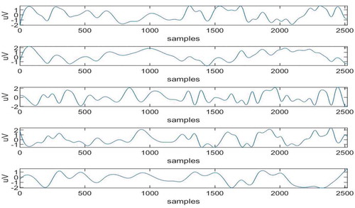
The maximum adjacent difference comes for 6^th in nature (Islam et al., 2016) and IMFs 1,2,3,4 and 5 are artifact-free IMFs. The artifactual IMFs that is IMFs 6,7,8,9,10 are given as input to ICA and corresponding 5 ICs are obtained as shown in Figure 5.

Figure 5. Independent components (ICs)

Now from these 5 ICS the artifactual ICs are selected. This is done using the concept of mMSE and kurtosis. The values of mMSE and kurtosis are calculated for each IC using formulas (9), (10), and (11). Threshold values of mMSE and kurtosis are also calculated using formulas (12) and (13). These values are denoted by Thresh1 = 0.1382 (for mMSE) and Thresh2 = 2.2955 (for kurtosis) and shown with red lines in Figure 6.

Figure 6. Kurtosis and mMSE for each IC with thresholds

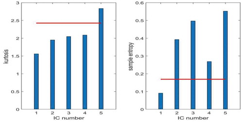
It can be clearly seen from Figure 6 that the value of kurtosis for 5^th IC is above threshold and value of mMSE for 1^st IC is below threshold. Hence, ICs 1 and 5 are considered to be artifactual in nature. So, constraints will be applied on columns of mixing matrix corresponding to these ICs.

As 5 artifactual IMFs are used as input signals of ICA and 5 ICs are obtained as output so it results in 5 × 5 mixing matrix with ICs. It can be observed from Figure 6 that 1^st and 5^th ICs are artifactual in nature so spatial constraints have to be applied on the first and fifth columns of given mixing matrix.

$A=\left[\begin{array}{cc}\begin{array}{ccc}-4.2394& 0.7226& -24.6049\end{array}& \begin{array}{cc}-20.8140& -2.8446\end{array}\\ \begin{array}{ccc}\begin{array}{c}-23.9179\\ 0.0485\\ \begin{array}{c}-3.6939\\ 4.9252\end{array}\end{array}& \begin{array}{c}5.9560\\ -3.6108\\ \begin{array}{c}0.3228\\ 16.2922\end{array}\end{array}& \begin{array}{c}1.5303\\ -7.8763\\ \begin{array}{c}-7.6902\\ -0.0910\end{array}\end{array}\end{array}& \begin{array}{cc}\begin{array}{c}-3.8094\\ 14.5854\\ \begin{array}{c}7.1017\\ 0.6771\end{array}\end{array}& \begin{array}{c}-5.7146\\ -19.3326\\ \begin{array}{c}9.8159\\ -1.2548\end{array}\end{array}\end{array}\end{array}\right]$

Now, the mixing matrix is modified by applying spatial constraints and it is given by

$\text{^}A=\left[\begin{array}{cc}\begin{array}{ccc}3.5865& 0.7226& -24.6049\end{array}& \begin{array}{cc}-20.8140& 10.1271\end{array}\\ \begin{array}{ccc}\begin{array}{c}3.4166\\ 3.6235\\ \begin{array}{c}3.5912\\ 3.6656\end{array}\end{array}& \begin{array}{c}5.9560\\ -3.6108\\ \begin{array}{c}0.3228\\ 16.2922\end{array}\end{array}& \begin{array}{c}1.5303\\ -7.8763\\ \begin{array}{c}-7.6902\\ -0.0910\end{array}\end{array}\end{array}& \begin{array}{cc}\begin{array}{c}-3.8094\\ 14.5854\\ \begin{array}{c}7.1017\\ 0.6771\end{array}\end{array}& \begin{array}{c}10.1168\\ 10.0683\\ \begin{array}{c}10.1722\\ 10.1327\end{array}\end{array}\end{array}\end{array}\right]$

As it can be clearly seen that 1^st and 5^th columns of the mixing matrix are modified. This modified mixing matrix is used with artifactual ICs and artifact-free ICs to obtain restored IMFs.

Figure 7. Restored IMFs

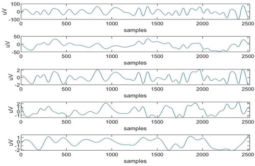
These restored IMFs shown in Figure 7 and the artifact-free IMFs that is IMFs 1,2,3,4,5 are added to obtain artifact-free EEG signal as plotted in Figure 8. Same process is repeated for EMD-ICA and EEMD-ICA and corresponding artifact-free EEG signals are obtained for comparison purpose.

It can be observed from Figure 8 that cascaded combination of EEMD and SCICA has led to removal of noise between 3^rd and 4^th sec and also between 7^th and 8^th sec. Now, the results are compared in terms of three parameters i.e. Mutual Information, Correlation, and Coherence. These parameters are calculated between real time EEG signal and the Artifact-free EEG signal. 10 real-time EEG signals from different databases are used here to verify results. The MI and Correlation Coefficients are calculated and shown in Tables 1 and 2 respectively.

Figure 8. Artifact-free EEG signals using EEMD-SCICA

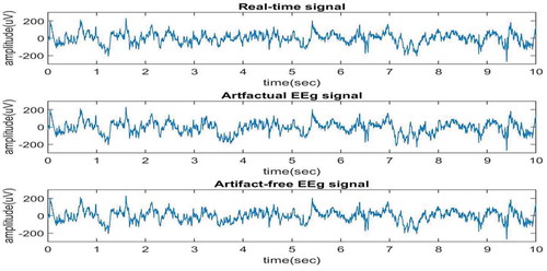
Table 1. Mutual information

Channel No.	Wavelet + ICA(Inuso, 2007)	Stationary Wavelet Enhanced ICA(Choudhry & Kapoor, 2016b)	EMD+ICA (Wang et al., 2016)	EEMD+ICA (Zeng et al., 2016)	Proposed Method (EEMD+SCICA)
1	0.4122	0.4850	0.4288	0.4601	0.4852
2	0.4982	0.6179	0.5094	0.5554	0.6273
3	0.7238	0.8998	0.7458	0.8094	0.9094
4	0.3756	0.6682	0.3812	0.6594	0.6691
5	0.3823	0.5489	0.3857	0.4259	0.5492
6	0.8098	0.9392	0.8223	0.8931	0.9402
7	0.6124	0.8762	0.6255	0.7826	0.8865
8	0.8359	0.9592	0.8463	0.9104	0.9724
9	0.7098	0.9128	0.7210	0.8425	0.9210
10	0.6206	0.8476	0.6608	0.7724	0.8545

Table 2. Correlation coefficient

Channel No.	Wavelet + ICA(Inuso, 2007)	Stationary Wavelet Enhanced ICA(Choudhry & Kapoor, 2016b)	EMD+ICA (Wang et al., 2016)	EEMD+ICA (Zeng et al., 2016)	Proposed Method (EEMD+SCICA)
1	0.8322	0.9182	0.8401	0.8766	0.9254
2	0.7654	0.9254	0.8635	0.8992	0.9305
3	0.8284	0.9262	0.8847	0.9196	0.9273
4	0.7468	0.8907	0.8032	0.8743	0.9097
5	0.8854	0.9671	0.8911	0.9336	0.9826
6	0.6974	0.9042	0.7828	0.8301	0.9194
7	0.8062	0.9167	0.8255	0.8641	0.9188
8	0.8209	0.9498	0.8852	0.9235	0.9504
9	0.8446	0.9432	0.8603	0.9004	0.9448
10	0.8247	0.9542	0.8722	0.9102	0.9611

From Tables 1 and 2, it can be seen that the value of MI and Correlation Coefficient are maximum for EEMD with SCICA for all channels. MI and Correlation Coefficient are maximum for 8^th channel and 5^th channel in case of proposed method. Coherences between Real-Time EEG signal and Artifact-free EEG signal of channel No 07 are plotted in Figure 9.

Figure 9. Coherence of EMD-ICA, EEMD-ICA and EEMD-SCICA

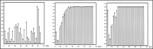
It can be observed from Figure 9 that the coherence is better for EEMD with SCICA as compared to other methods.

5. Conclusion

The proposed method improves results of ocular artifact removal from real-time artifactual EEG signal by using strengths of both EEMD and SCICA. EEMD is used to decompose the EEG signal into IMFs, which results in more efficient functioning of ICA by ensuring that the number of observed sources or input signal to ICA (here IMFs) is more than or equal to independent sources (here ICs). EEMD is also used to overcome the mode mixing and aliasing problem of EMD. Effect of artifact in IMFs is reduced by applying spatial constraints in columns of mixing matrix of ICA. Here, performance of proposed method is compared with other state-of-the-art methods in terms of Correlation Coefficient, Mutual Information and Coherence. Correlation Coefficient and Mutual Information are used to verify performance of proposed method in time domain and Coherence is plotted to measure performance in frequency domain. For the future scope, EEMD can be replaced by CEEMD to overcome amplitude reduction problem of EEMD. The performance can be further improved by applying some better constraints on ICA and also by using wavelet enhanced independent component analysis (Issa & Juhasz, 2019).

Additional information

Funding

The authors received no direct funding for this research.

Notes on contributors

Anchal Yadav

Anchal Yadav was born in Noida, India, in 1993. She received her B.Tech. degree from J.S.S.A.T.E., Abdul kalam Technical University, U.P., India and M.TECH. degree from Delhi Technological University, Delhi, India, in 2015 and 2018, respectively. She is currently working towards the Ph.D degree in EEG-Source Localization at Indian Institute of Technology, Delhi, India. Her interest is in working in localizing the activity in the brain using brain signals. Since ocular artifact (artifact due to eye-blink and eye movement) cannot be avoided while recording EEG from patients especially in young children. Our paper “A New Approach for Ocular Artifact Removal from EEG Signal using EEMD and SCICA” provides a good and easy method to eradicate ocular artefacts from EEG signal. This method can be used in the pre-processing step and artifact-free data can be obtained for further analysis.

Mahipal Singh Choudhry is an Associate Professor in the Department of Electronics and Communication of Delhi Technological University (DTU), India. He completed his B.tech and M.tech in Electronics and Communication from M.NIT Jaipur, India, and completed his Ph.D. from DTU, India. His interested areas of research are Biomedical Signal Processing and Biomedical Image Processing.

References

- Benbadis, S. R., & Rielo, D. A. (2008). EEG Artifacts Overview. http://emedicine.medscaple.com/article/1140247-overview
- Bosl, W., Tierney, A., Flusberg, H. T., & Nelson, C. (2011). EEG complexity as a biomarker for autism spectrum disorder risk. BMC Medicine, 9(1), 1–17. https://doi.org/10.1186/1741-7015-9-18
- Choudhry, M. S., & Kapoor, R. (2016a, October). Removal of baseline wander from ECG using CEEMD and adaptive morphological function. Journal of Chemical and Pharmaceutical Sciences, 974-2115.
- Choudhry, M. S., & Kapoor, R. (2016b). Ocular artifact removal from EEG using stationary wavelet enhanced ICA. International Journal of Control Theory and Applications, 9(10), 4935–4945.
- Devulapalli, S. P., Rao, C. S., & Prasad, K. S. (2019, May). Eye-blink artifact removal of EEG signal using EMD. International Journal of Recent Technology and Engineering (IJRTE).
- Hagemann, D., & Naumann, E. (2001). The effects of ocular artifacts on (lateralized) broadband power in the EEG. Clinical Neurophysiology, 112 (2), 215–231. https://doi.org/10.1016/S1388-2457(00)00541-1.
- Hesse, C. W., & James, C. J. (2005). The FastICA algorithm with spatial constraints. IEEE Signal Processing Letters, 12(11).
- Huang, N., Shen, Z., Long, S.R., Wu, M.C., Shih, H.H., Zheng, Q., Yen, N.C., Tung, C.C., &, Liu, H.H. (1998). The empirical mode decomposition and the Hilbert spectrum for nonlinear and non-stationary time series analysis. Proceedings of the Royal Society A: Mathematical, Physical and Engineering Sciences, 454(1971), 995, 903.
- Ille, N. (2001). Artifact correction in continuous recordings of the electro- and magnetoencephalogram by spatial filtering [Ph.D. dissertation].
- Inuso, G. (2007, August) Wavelet-ICA methodology for efficient artifact removal from Electroencephalographic recordings. In Proceedings of International Joint Conference on Neural Networks (pp. 12–17). Orlando-USA.
- Islam, M. K., Rastegarnia, A., & Yang, Z. (2016). Methods for artifact detection and removal from scalp EEG: A review. Neurophysiologie Clinique/Clinical Neurophysiology, 46(4–5), 287–305. https://doi.org/10.1016/j.neucli.2016.07.002
- Issa, M. F., & Juhasz, Z. (2019, December). Improved EOG artifact removal using wavelet enhanced independent component analysis. Journal of Brain Science, 9(12), 355. https://doi.org/10.3390/brainsci9120355
- James, C. J., & Hesse, C. W. (2006, December). On semi-blind source separation using spatial constraints with applications in EEG analysis. IEEE, Trans. On Biomed. Eng., 53(12).
- Jiang, X., Bian, G.-B., & Tian, Z. (2019, February). Removal of artifacts from EEG signals: A review. Sensors.
- Joyce, C. A., Gorodnitsky, I. F., & Kutas, M. (2004). Automatic removal of eye movement and blink artifacts from EEG data using blind component separation. Psychophysiology, 41(2), 313–325. https://doi.org/10.1111/j.1469-8986.2003.00141.x
- Jung, T. P., Humphries, C., Lee, T. W., Makeig, S., McKeown, M. J., Iragui, V., & Sejnowski, J. (1998). Extended ICA removes artifacts from EEG recordings. Advances in Neural Information Processing Systems, 10, 894–900.
- Mahajan, R., & Morshed, B. I. (2015, January). Unsupervised eye blink artifact denoising of EEG data with modified multiscale sample entropy, kurtosis and wavelet-ICA. IEEE Journal of Biomedical and Health Informatics, 19(1), 158–165. https://doi.org/10.1109/JBHI.2014.2333010
- Makeig, S., Bell, A. J., Jung, T. P., & Sejnowski, T. J. (1996). ICA of Electroencephalographic Data. Advances in Neural Information Processing Systems, 8, 145–151.
- Pramudita, B. A., Nugroho, Y. D., Ardiyanto, I., Shapiai, M. I., & Setiawan, N. A. (2017, November). Removing ocular artefacts in EEG signals by using combination of complete EEMD (CEEMD)- independent component analysis (ICA) based outlier data. In IEEE International Conference on Robotics, Automation and Science (ICORAS). (pp. 27–29) Malaysia.
- Rilling, G., Flandrin, P., & Es, P. (2003). On empirical mode decomposition and its algorithms. In IEEE-EURASIP Work. nonlinear signal image process (vol. 3, pp. 8–11).
- Wang, G., Teng, C., Kuo, L., Zhang, Z., & Yan, X. (2016, September). The removal of EOG artifacts from EEG signals using independent component analysis and multivariate empirical mode decomposition. IEEE Journal of Biomed. And Health Inf, 20(5).
- www.physionet.org
- Zeng, K., Chen, D., Ouyang, G., Wang, L., Liu, X., & Xiaoli, L. (2016, June). An EEMD-ICA approach to enhancing artifact rejection for noisy multivariate neural data. IEEE Transactions on Neural Systems and Rehabilitation Engineering, 24(6), 630–638. https://doi.org/10.1109/TNSRE.2015.2496334
- Zhaohua, W., & Huang, N. E. (2005, August). Ensemble empirical mode decomposition: A noise assisted data analysis method [Thesis].