Modeling and control of a 3-DOF articulated robotic manipulator using self-tuning fuzzy sliding mode controller

Abstract

Robotic manipulators are highly coupled multi-input multi-output (MIMO) nonlinear systems with uncertainties and highly time-varying dynamic capabilities. These characteristics make the trajectory control of a robotic manipulator very challenging. This paper presents the modeling and trajectory tracking control of a 3-DOF robotic manipulator using self-tuning fuzzy sliding mode controller (ST-FSMC). The stability of the system was investigated using the Lyapunov direct method. The controller was implemented using MATLAB/Simulink and its performance was evaluated. The simulation results show that the proposed controller removed chattering phenomena from the control effort and reduced the tracking error (average steady-state error) to 0.0036 rad. However, in the case of the conventional controllers, the average steady-state e rror increased to 0.0413 rad, 0.0044 rad, and 0.0053 rad for the Proportional-integral-derivative (PID) controller, Sliding mode controller (SMC), and Fuzzy sliding mode controller (FSMC), respectively. The conventional controllers (PID, SMC, and FSMC) were designed for the purpose of comparison with the proposed ST-FSMC. The simulation results show that the designed controller (ST-FSMC) has a superior tracking performance, is robust and is not sensitive to applied model parameter variations as compared to other conventional controllers.

Keywords:

• Fuzzy sliding mode controller
• sliding mode controller
• ST-FSMC
• PID
• DOF

PUBLIC INTEREST STATEMENT

Robots are in widespread use in recent times. This is because most industries make use of robots to increase productivity and product quality. Robots are also used to get jobs done faster with greater precision and reliability than humans. Robot manipulators are created from a sequence of link and joints. They are highly complicated nonlinear systems with uncertainties. These characteristics make the trajectory control of a robotic manipulator difficult. To solve the problem of handling uncertainties with the aim of increasing the robustness of the system to give an improved output, a self-tuning fuzzy sliding mode controller (ST-FSMC) was proposed. This control method was implemented to give a high-performance controller in the presence of uncertainties. In addition, various control methods were successfully designed and comparative analysis was carried out. Simulations were performed to demonstrate that the proposed ST-FSMC performances better than other conventional controllers (PID, SMC, and FSMC) because the proposed controller can adjust itself to the systems uncertainty.

1. Introduction

Robots are in widespread use in recent times to get jobs done faster with greater precision and reliability than humans. Nowadays, most industries make use of robots to increase productivity, precision, and product quality. A robot makes use of a robotic manipulator to perform tasks which are most times difficult to perform. These tasks include: space exploration, robotic surgery or welding. The robotic manipulator is an electrically actuated Three Degrees of Freedom (3-DOF) arm-like serial manipulator comprising several segments which may be sliding or jointed. They are used in industrial applications with articulated geometric types because articulated robotic manipulators are most commonly used in factories worldwide (Gambhire et al., 2021).

Articulated manipulators are the most common industrial robotic structures providing more than 50% of annual installations around the world (Wang et al., 2014). This type of robot is utilized in numerous industrial processes such as welding, painting, pick and place, dispensing, packaging as well as several handling applications which include machine tool tending, metal casting, and general material handling. It has a wide workspace and operates in a 3-D space.

Robotic manipulators are also employed for jobs that are too dirty, hazardous, and highly repetitive or boring to be suitable for humans (Ghaleb & Aly, 2018). Due to these reasons, robotic manipulator research is one of the most interesting areas in industrial technology applications. However, most of these applications are confined to slow motion operations without interactions with the environment. This is primarily due to the limited performance of the available controllers in the market. To help improve the operational speed for better accuracy, advanced control strategies are required. Because a controller is the main part of this sophisticated system, the main requirements to control robotic manipulators are stability and robustness. The main challenges in its motion and control are the complexity of its dynamics and the presence of uncertainties in the system. Consequently, modeling and analysis of a robotic manipulator and in addition implementing control methods are significant to obtain precision, good accuracy, and increased productivity.

This paper presents the modeling and design of a controller for a 3-DOF robotic manipulator which requires minimum effort with a minimum error. Since, trajectory-tracking control of robotic manipulators is a challenging task due to the highly coupled MIMO and highly time-varying dynamic nature of the system. Furthermore, there are always numerous uncertainties in the system model such as parameter uncertainty and external disturbance which cause unstable performance of the control system. In addition to this, most research works have been observed to neglect actuator dynamics. This resulted in reduced trajectory tracking control performance. In any control system, stability and robustness are the two important characteristics that a robot manipulator requires. Consequently, it is very important to model and evaluate robot manipulators by utilizing proper control methods. In industrial applications, typical PID controllers are used to control such complex systems. PID controllers are easy to implement and require the tuning of only three parameters, and have relatively acceptable tracking performance for a robot. But the linear PID controller is not suitable to accomplish the desired tracking performance of nonlinear dynamic systems.

Different researches have been done to reduce the shortcomings of PID control using a nonlinear controller, and in addition, different approaches have been proposed for designing nonlinear controllers such as FLC, SMC, and FSMC. All these three controllers have been applied successfully in many applications, but they also have some limitations. Therefore, this paper also addresses the problem of performance degradation or loss of system stability due to neglected actuator dynamics by taking into account actuator dynamics in the system to improve the performance response.

2. Related works

Various modeling and control strategies have been presented in different researches for trajectory tracking control of robotic manipulators. In this section, a review of the researches which focus on trajectory-tracking control of robotic manipulators and other related controllers used in the control of robot manipulator systems is presented. In general, the studies in the literature reviewed in this paper focused on modeling and design of the system for either a linear or a nonlinear controller.

In Ohri et al. (2011), the authors present a comparison of the conventional PID controller and sliding mode control (SMC) for robotic manipulators. Both techniques have good performance, but the SMC is insensitive to parametric variations and has good disturbance rejection. The simulation results of the study show that the performance of the SMC is better than PID under both sine and cosine trajectory. As the payload is changed or during uncertainty, the tracking error in the PID controller is increased, but in the case of SMC, the performance remains the same, which clearly shows that the SMC is more robust than the PID controller. In this paper, the authors assume that the actuators do not have dynamics of their own, and arbitrary forces can be commanded at the joint of the robotic manipulator for simplicity. The results obtained were promising, but the authors didn’t consider the actuator dynamics and ignored the effects of joint friction which brought about low controller performance.

In Getachew (2018), the authors proposed SMC for a two degrees of freedom (2-DOF) robotic manipulator system and presented a comparative study of PID controllers. Based on simulation results and analysis, the authors concluded that the SMC controller has superior performance and is more robust when contrasted with the PID controller for sinusoidal trajectory tracking. The results obtained show a good performance response when the system is under a disturbance of 25% of the input amplitude. The problem with this was, as the system disturbance increased to 40% of the input amplitude, the sliding surface and the derivative of the sliding surface of the second joint introduced a chattering which caused a chattering in the control effort of the second joint. Finally, the authors suggested that in future works, other chattering elimination methods can be designed which may overcome any amount of disturbance introduced in the robot.

In Alassar et al. (2010), the authors introduced a fuzzy logic controller (FLC) for manipulating a 5-DOF robotic manipulator based on the independent joint control approach. The proposed controller was developed to overcome the shortcomings of the linear PID controller. Simulation was performed using MATLAB/Simulink to compare the performance of the controller in terms of time response. The results obtained were promising as the FLC was used to control complex nonlinear dynamic systems. However, the design of the FLC highly depended upon expert knowledge or trial and error. Furthermore, it didn’t guarantee stability and robustness due to the linguistic expressions of fuzzy control.

A design of computed torque control (CTC) methodology for PUMA-560 robot manipulator was presented in (Piltan et al., 2012a). Computed torque control (CTC) is a powerful nonlinear controller that is extensively utilized in robot manipulator control which calculates the required torques for all manipulator joints using a nonlinear feedback control law based on feedback linearization. The simulation results indicate that the CTC controller works very well when all dynamic and physical parameters are known. But still, there was a problem in uncertain dynamic system models. In most physical systems like robot manipulators, the parameters are unknown or time-variant. Consequently, the authors recommended designing a sliding mode controller (SMC) to solve this problem.

In (Piltan et al., 2012b), a novel fuzzy sliding mode controller (FSMC) was introduced to control the bus suspension system by combining fuzzy logic with an SMC. This method eliminates the two major drawbacks of SMC; firstly by using the boundary layer instead of the signum and FLC in place of the equivalent dynamic part of SMC to eliminate the chattering and equivalent dynamic dependency problem, respectively. The authors concluded from the outcome of the simulation that FSMC has better performance for the bus suspension system and is more robust as compared to the PID controller.

In Rahmdel et al. (2012), the authors introduced an intelligent control approach called the FSMC with global stabilization and saturation function (boundary layer method) for the trajectory tracking control of a robot manipulator. The FSMC used in their work has to chatter in it. This chattering effect of the FSMC was eliminated by applying a saturation function instead of a signum function. The authors used several conventional methods such as PD, CTC, and SMC to evaluate and contrast the proposed control method. Finally, the results of the simulation indicate that the FSMC can guarantee robustness against continuous disturbance and has a strong ability to eliminate chattering.

A nonlinear SMC was utilized in a spread-out scope of regions such as in robotics, process control, and aerospace applications in Shaei (2010). The main reason this controller was used is because of its performance. Also it solves some main challenging issues in the systems control such as resistivity to external disturbance and uncertainty. However, this controller has two significant limitations: the chattering and sensitivity problem; therefore the controller is very sensitive to noise. In Chang et al. (2008), an SMC with a boundary layer technique to minimize or eliminate chattering was presented. In the boundary layer technique, the basic idea is to replace the saturation function with a discontinuous function in a small neighborhood of the switching surface. But, this replacement caused an increase in the error performance, and also increased the rising time. Similarly, in Kapoor & Ohri (2013), the authors presented an SMC with saturation and hyperbolic tangent functions instead of signum function. Unfortunately, this approach was effective only in specific cases. When hard uncertainties are not present, some problems are attenuated at the cost of a loss of robustness. Furthermore, a nonlinear FSMC was used to reduce or compensate the negative effect of saturation function in the system. However, both SMC and FSMC have difficulty in handling unstructured model uncertainties, because the sliding surface gain is chosen by trial and error, which means that the SMC and FSMC must have prior knowledge of the systems uncertainty. In contrast to other papers, this work combines the fuzzy-based tuning method with FSMC to overcome the problem of handling unstructured model uncertainties to increase the robustness of the system. The fuzzy-based tuning method was used to adjust the sliding surface slope (λ) as well as a switching gain (K) to obtain the best performance of the system. The coefficients which have a significant impact on the discontinuous part of the control system were investigated. If these coefficients are tuned properly, the SMC can reject disturbances more desirably. Accordingly, the proposed controller (Self-tuning-FSMC) has powerful resistance and can solve the problems of both structured and unstructured uncertainties (Kapoor & Ohri, 2017; Medhaar et al., 2006). In (Anh et al., 2018), an adaptive fuzzy sliding mode controller (AFSMC) to demonstrate the stability of a robotic manipulator system using Lyapunov stability theorem was presented. Similarly, an AFSMC was proposed in (Zhang et al., 2020) to improve the trajectory tracking accuracy of a 3-DOF serial manipulator with parameters uncertainties.

Past researches on the design of various control techniques indicate that actuator dynamics plays an important role in the overall robot dynamics and poor attention to this aspect may cause imperfection in the final control system, particularly in the case of high-velocity moment, and highly varying loads as reported in Tao & Lee (2016). Moreover, the saturation of the actuator was not given much attention in the dynamic modeling of the robot manipulator. The authors used an electrical actuator to drive all joints of the robot manipulator, and the injected force/torque of the joints is the load torque of the actuator, which is considered in the dynamic model of the overall system. Additionally, in the case of torque-based control design, the torque directly controls the actuators which cause them to face implementation issues in real-time applications (Karamali Ravandi et al., 2018). On the other hand, the voltages of the electrical actuators are utilized to control commands in practical applications. In (Dhyani et al., 2020), the authors presented a redundant 7-DOF manipulator. It possesses more resources than those strictly required to execute a given task. This provides the robot manipulator with an increased capacity to work in real-world applications. However, the inverse kinematics and control of redundant manipulators are becoming increasingly complicated with each added degree of freedom. In addition, the system dynamics are complex and may involve un-modelled uncertainties; thereby causing the corresponding path planning problem to become increasingly challenging.

To address these challenges, this paper proposes a self-tuning fuzzy slide mode controller (ST-FSMC) with powerful resistance to solve both structured and unstructured uncertainty problems. In addition, the paper also addresses the problem of performance degradation or loss of system stability due to neglected actuator dynamics by taking into account actuator dynamics in the system to improve the performance response. To meet the predefined aim of this paper, authors primarily concentrated on the study of the literature about the theoretical and structural background of the robotic manipulator and its controller. Thereafter with the knowledge gained, we have compared the performance of various controllers with the aim of overcoming the shortcomings of the traditional linear and nonlinear controllers with the proposed controller (ST-FSMC).

Since the appropriate dynamic model equations are very important in designing the robotic controller, to develop the model we have divided the developmental stages into two main parts. First, we developed the robot manipulator dynamic equations. This starts from the equation of position and orientation description, forward and inverse kinematics, dynamic analysis and forces, kinematic and potential energy derivations using the Lagrange equation. The second is to model the actuator dynamics of the robot with some assumptions.

Finally, the overall nonlinear system model or manipulator and actuator dynamics are developed. Since in most of the past studies, the control input is a torque or force but in our case, instead of using torque or force, we used the voltage of the actuator from the developed mathematical model. This was done to improve the drawbacks noticed in previous works.

After the dynamic models have been developed, the proposed controller (Self-Tuning FSMC) for a 3-DOF robot manipulator was designed with MATLAB. Finally, the performance of the proposed method is tested and compared with the conventional controller by simulation using MATLAB software, and then analysis and interpretation of the results of simulation were presented.

3. Dynamic and kinematic formulation of 3-DOF articulated robotic manipulator

The first important step in controlling any physical system is to acquire a complete and accurate mathematical model of the system. This model is useful for simulation of the system before implementing the system into a real-time application. In this section, the mathematical equations for the kinematic and dynamic model of the three-link industrial robotic manipulator having three revolute joints are discussed. The kinematic analysis has been classified into two types, forward and inverse kinematics, and the dynamic behavior of the manipulator concerned with the relationship between joint actuator torques and motion of links for the design of the control algorithms.

Finally, the overall nonlinear system model or manipulator dynamic and actuator dynamics are developed. Since most of the literatures have presented the use of the control input, torque or force, but in our case, instead of these, we used the voltage of the actuator from the developed mathematical model. This is to improve on some of the drawbacks in the previous works.

3.1. Kinematic modeling of robot manipulator

Kinematics describe and analyze the motion of bodies without regard to forces or moments that cause the motion. In kinematics, the position, orientation, velocity, and acceleration of the robot manipulator are analyzed from the point of spatial geometry. To describe the geometry, a link frame based on Denavit-Hartenberg (DH) description is assigned to each link of the manipulator. The kinematics are divided into forward (FK) and Inverse (IK) kinematics.

The forward kinematics is done using the Denavit–Hartenberg (DH) parameters. The DH parameters use only four factors which describe the movement of the robotic manipulator. These parameters are:$q$is the rotation angle: this is along z-axis always,$\alpha$ is twist: this is the angle it takes to map z-axis of the previous joint to the current joint,$a$is the distance of previous joint center to next center in x-direction and $d$ is the offset distance of previous joint center to next in z-direction.

The frame assignments for the 3-DOF articulated robotic arm showing the various joints and their links are shown in Figure 1 (Massaoudi et al., 2019). The DH parameters for the 3-DOF robotic manipulator are presented in Table 1.

Figure 1. Frame assignments for the 3-DOF articulated robotic arm

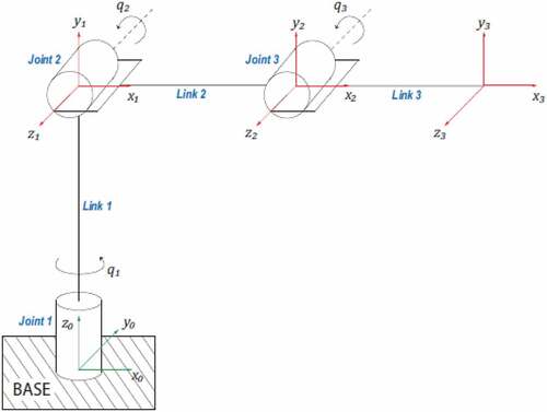
Table 1. DH parameter for 3-DOF articulated robotic arm

Link	$a_{i-1}$	${\alpha }_{i-1}$	$d_i$	$q_i$
1	0	${90}^0$	$L_1$	$q_1$
2	$L_2$	0	0	$q_2$
3	$L_3$	0	0	$q_3$

Subsequent to getting the DH-convention table, a series of homogeneous matrices are obtained based on the number of the DOF. Therefore, the overall homogeneous transformation matrix for the position and orientation of the end effector that is required is given as:

(4) $T_0^3=\left[\begin{array}{cccc}{C}_1{C}_{23}& -C_1{S}_{23}& S_1& L_3{C}_1{C}_{23}+L_2{C}_1{C}_2\\ S_1{C}_{23}& -S_1{S}_{23}& -C_1& L_3{S}_1{C}_{23}+L_2{S}_1{C}_2\\ S_{23}& C_{23}& 0& L_3{S}_{23}+L_2{S}_2+L_1\\ 0& 0& 0& 1\end{array}\right]$(4)

The homogenous transformation matrix defined in Eq. (4)(4) $T_0^3=\left[\begin{array}{cccc}{C}_1{C}_{23}& -C_1{S}_{23}& S_1& L_3{C}_1{C}_{23}+L_2{C}_1{C}_2\\ S_1{C}_{23}& -S_1{S}_{23}& -C_1& L_3{S}_1{C}_{23}+L_2{S}_1{C}_2\\ S_{23}& C_{23}& 0& L_3{S}_{23}+L_2{S}_2+L_1\\ 0& 0& 0& 1\end{array}\right]$(4) is the one that defines the forward kinematics of the 3-DOF robotic manipulator shown in Figure 1. From this matrix, the position and orientation of end effectors is a non-linear function of joint variables. Having derived the forward kinematics of Figure 1, then it’s possible to obtain the position and orientation of the end-effector from the individual joint angle ($q_1$,$q_2,and$$q_3$). The end-effector orientation matrix is represented by the first three rows and columns of the transformation matrix in Eq. (5)(5) $\left\{\begin{array}{c}{p}_x=L_3{C}_1{C}_{23}+L_2{C}_1{C}_2\\ p_y=L_3{S}_1{C}_{23}+L_2{S}_1{C}_2\\ p_z=L_3{S}_{23}+L_2{S}_2+L_1\end{array}\right\},R_d=\left[\begin{array}{ccc}{C}_1{C}_{23}& -C_1{S}_{23}& S_1\\ S_1{C}_{23}& -S_1{S}_{23}& -C_1\\ S_{23}& C_{23}& 0\end{array}\right]$(5) .

(5) $\left\{\begin{array}{c}{p}_x=L_3{C}_1{C}_{23}+L_2{C}_1{C}_2\\ p_y=L_3{S}_1{C}_{23}+L_2{S}_1{C}_2\\ p_z=L_3{S}_{23}+L_2{S}_2+L_1\end{array}\right\},R_d=\left[\begin{array}{ccc}{C}_1{C}_{23}& -C_1{S}_{23}& S_1\\ S_1{C}_{23}& -S_1{S}_{23}& -C_1\\ S_{23}& C_{23}& 0\end{array}\right]$(5)

3.2. Inverse kinematics

The inverse kinematics of the robotic manipulator are a way of finding the robot manipulator joint variables given the position of the Cartesian coordinates of the end-effector. In this section, we solved the inverse kinematics equations for the 3-DOF robotic manipulator using the geometrical approach as given by Eqs. (6)(6) $p_x^2+p_y^2>0$(6) -(8)

$q_1=aarctan(p_y,p_x)$, where, $q_1$ is defined only when

(6) $p_x^2+p_y^2>0$(6)

$q_3=atan2(S_3,C_3)$, where,$C_3=\frac{p_x^2+p_y^2+{(p_z-1)}^2-l_2^2-l_3^2}{2l_2{l}_3}$,$S_3=\pm \sqrt{1-{C_3}^2}$ (7)

$S_3\in [-0.173,0.173]$ (Else, point P (end effector point) is out of workspace). This is due to joint three constraint.

$q_2=atan2(S_2,C_2)$, where, $q_2$ is defined if and only if $p_x^2+p_y^2+(p_z-1{)}^2>0$

$S_2=\frac{(l_2+l_3{C}_3)(p_z-l_1)-l_3{S}_3(C_1{p}_x+p_y{S}_1)}{{l_3}^2{S_3}^2-{(l_2+l_3{C}_3)}^2}$, $C_2=\pm \sqrt{1-{S_2}^2}\in [-1,1]$ (8)

3.3. Dynamic model of 3-DOF robotic manipulator

In this section, we derive the mathematical equations that explicitly describe the relationship between the joint torques applied by the actuators and motion of the robot system. The best technique that can be used for obtaining the dynamic model of the manipulator is the Euler-Lagrangian approach which gives an energy difference between the kinetic energy and potential energy. This approach is mostly used in deriving the complicated mathematical model of a robot manipulator (Abbas, 2018). Therefore, we have used the Euler -Lagrange method in this paper.

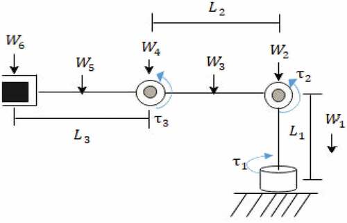
Therefore, kinetic and potential energy analysis of each link of the manipulator must be carried as shown in Figure 2. The kinetic energy can be both rotational and translational; it is a function of both position and velocity, $K_E(q,\dot{q})$. The potential energy is due to conservative forces exerted by gravity. The Euler-Lagrange equations for the n-DOF system are defined as:

(9) $\frac{d}{d_t}(\frac{\mathrm{\partial }L(q,\dot{q})}{\mathrm{\partial }{q}_i})-\frac{\mathrm{\partial }L(q,\dot{q})}{\mathrm{\partial }{q}_i}={\tau }_i$(9)

Figure 2. Force calculation of joints

where, $i=1,2\dots .n,$ ${\tau }_i$ is the torque/ force exerted on each joint of the manipulator, $q_i$is the link position, and ${\dot{q}}_i$is the joint velocity.

The values of the physical parameters of the manipulator are presented in Table 2 (Korayem et al., 2010; Pezeshki et al., 2012).

Table 2. List of parameters of robot manipulator

Parameter	Notation	Value
Length of link 1	$l_1$	0.15 m
Length of link 2	$l_2$	0.5 m
Length of link 3	$l_3$	0.5 m
Mass of link 1	$m_1$	0.5 kg
Mass of link 2	$m_2$	0.5 kg
Mass of link 3	$m_3$	0.5 kg
Gravity	$g$	$9.81m/s^2$

As there are 3-DOF, the Euler-Lagrangian equations give these three equations (Eqs. (10(10) $\begin{array}{rl}& {\tau }_1=(\frac{1}{2}{m}_1{r}_1^2+\frac{1}{4}{m}_2{l}_2^2{C}_2^2+\frac{1}{4}{m}_3{l}_3^2{C}_{23}^2+m_3{l}_2^2{C}_2^2+m_2{l}_2{l}_{23}{C}_2{C}_{23}){\ddot{q}}_1+(-\frac{1}{4}{m}_2{l}_2^{2}sin(2q_2)-m_3{l}_2^{2}sin(2q_2)\\ & -m_3{l}_2{l}_{3}sin(2q_2+q_3)-m_3{l}_{c2}^{2}sin(2(q_2+q_3))){\dot{q}}_1{\dot{q}}_2+(-m_3{l}_2{l}_3{C}_2{S}_{23}-m_3{l}_{c3}^{2}sin(2(q_2+q_3)){\dot{q}}_1{\dot{q}}_3\end{array}$(10) )–(12(12) ${\tau }_3=\frac{1}{3}{m}_3{l}_3^2{\ddot{q}}_3-m_3(l_2{l}_{c3}{C}_3+l_{c3}^2){\ddot{q}}_2+m_3{l}_{c3}{S}_{23}(l_2{C}_2+l_{c3}{C}_{23}){{\dot{q}}_2}^2+m_3(l_2{l}_{c3}S{\dot{q}}_2{\dot{q}}_3+g{l}_{c3}{C}_{23})$(12) )).

(10) $\begin{array}{rl}& {\tau }_1=(\frac{1}{2}{m}_1{r}_1^2+\frac{1}{4}{m}_2{l}_2^2{C}_2^2+\frac{1}{4}{m}_3{l}_3^2{C}_{23}^2+m_3{l}_2^2{C}_2^2+m_2{l}_2{l}_{23}{C}_2{C}_{23}){\ddot{q}}_1+(-\frac{1}{4}{m}_2{l}_2^{2}sin(2q_2)-m_3{l}_2^{2}sin(2q_2)\\ & -m_3{l}_2{l}_{3}sin(2q_2+q_3)-m_3{l}_{c2}^{2}sin(2(q_2+q_3))){\dot{q}}_1{\dot{q}}_2+(-m_3{l}_2{l}_3{C}_2{S}_{23}-m_3{l}_{c3}^{2}sin(2(q_2+q_3)){\dot{q}}_1{\dot{q}}_3\end{array}$(10)

(11) $\begin{array}{rl}& {\tau }_2=(\frac{1}{4}{m}_2{l}_2^2+m_3(l_2^2+l_{c3}^2+l_2{l}_3{C}_3)){\ddot{q}}_2-m_2{l}_2{l}_3{S}_3{\dot{q}}_2{\dot{q}}_3+m_3(l_2{l}_{c3}{C}_3+l_{c3}^2){\ddot{q}}_3-m_3{l}_2{l}_{c3}{S}_3{\dot{q}}_3+\\ & (\frac{1}{2}{m}_2{l}_{c2}^{2}sin(2q_2)+m_3\frac{l_2^2}{2}sin(2q_2)+l_2{l}_{c3}{m}_{3}sin(2q_2+q_3)+\frac{1}{2}{l}_{c3}^{2}sin2(q_2\\ & +q_3)){\dot{q}}_1^2+l_{C2}{m}_{2}g{C}_2+l_2{m}_{3}g{C}_2+l_{C3}{m}_{2}g{C}_{23}\end{array}$(11)

(12) ${\tau }_3=\frac{1}{3}{m}_3{l}_3^2{\ddot{q}}_3-m_3(l_2{l}_{c3}{C}_3+l_{c3}^2){\ddot{q}}_2+m_3{l}_{c3}{S}_{23}(l_2{C}_2+l_{c3}{C}_{23}){{\dot{q}}_2}^2+m_3(l_2{l}_{c3}S{\dot{q}}_2{\dot{q}}_3+g{l}_{c3}{C}_{23})$(12)

According to Euler-Lagrange’s equation, the 3-DOF robotic manipulator dynamics are given by three coupled nonlinear differential equations of motion. Presenting this in vector form, we obtain Eq. (13)(13) $\tau =M(q)\ddot{q}+B(q)[\dot{q},\dot{q}]+C(q)[\dot{q}{]}^2+G(q)$(13) .

(13) $\tau =M(q)\ddot{q}+B(q)[\dot{q},\dot{q}]+C(q)[\dot{q}{]}^2+G(q)$(13)

where, τ is the actuator’s torque vector,$M(q)$is $nxn$ symmetric and positively defined inertia matrix, $i.e$$M(q)=M(q{)}^T>0$, $B(q)$ is coriolis torque matrix, and $C(q)$ is centrifugal torque matrix, and $G(q)$ is the force of gravity, and is an n × 1 matrix, $q$is an n × 1 vector, $[\dot{q},\dot{q}]$is the vector of joint velocity and $[\dot{q}{]}^2$ is the derived vector given by: $[{{\dot{q}}^2}_1,{{\dot{q}}^2}_2,{{\dot{q}}^2}_3{]}^T$(Pezeshki et al., 2012).

In order to obtain the dynamic equations that reflect the reality of the physical system, it is essential to model (at least approximately) the forces of friction (Craig, 2009). Friction phenomena in robot manipulators may affect the accuracy of the system for position control, especially when the manipulator is moving at low velocities. For most engineering applications, a static friction model is sufficient; experimental works proved that a good static friction model can approximate the actual frictional forces with 90% of conformability (Marton & Lantos, 2007).

To simplify the model, the friction model consists of only the coulomb and viscous terms. Thus, this simplified friction model is known as a classic friction model. The advantage of this model is its simplicity with only two parameters. It can be described using Eq. (14(14) $F(\dot{q})=F_V\dot{q}+F_{S}sgn(\dot{q})$(14) ) (Bittencourt, 2007).

(14) $F(\dot{q})=F_V\dot{q}+F_{S}sgn(\dot{q})$(14)

where, $F(\dot{q})$ is the friction force, $F_S$ represents the direction-dependent Coulomb friction coefficient, $F_V$ is the viscous damping coefficient, and $\dot{q}$ is the velocity of the system.

The manipulator is subjected to external disturbances and approximate friction (Fateh, 2008). Eq. (13)(13) $\tau =M(q)\ddot{q}+B(q)[\dot{q},\dot{q}]+C(q)[\dot{q}{]}^2+G(q)$(13) is modified to give Eq. (15)(15) $\tau =M(q)\ddot{q}+B(q)[\dot{q},\dot{q}]+C(q)[\dot{q}{]}^2+G(q)+F(\dot{q})+{\tau }_d$(15) which includes friction ($F(\dot{q})$), external dynamics, and other terms as a global uncertainty term denoted by vector (${\tau }_d$).

(15) $\tau =M(q)\ddot{q}+B(q)[\dot{q},\dot{q}]+C(q)[\dot{q}{]}^2+G(q)+F(\dot{q})+{\tau }_d$(15)

3.4. Overall system model including actuators

In a number of literatures, the design of a controller for the robot manipulator control system without introducing the actuator dynamics has been presented (Hu & Woo, 2006; Wai, 2003), while actuator dynamics plays an important role in the overall robot dynamics. Proper selection of actuators will dictate how effectively a robot can perform a specific task.

3.4.1. Joint torque calculations

Selecting the right motor for the joint is not a random selection. It was done based on calculations of expected weights that each joint will handle. The basic specification we look for when selecting a motor for a joint is the holding torque. For the motor to be able to hold the link and all subsequent links connected to it. To estimate the torque required at each joint, the worst-case scenario must be chosen. The diagram to represent this is shown in Figure 2.

where, $W_1$, $W_3$, and $W_5$are the weights of link one, two, and three respectively. The effecting point of those weights is at the center of each link. $W_2$and $W_4$ are the weights of the second and third joint (motor at each joint was also taken into account). $W_6$is the maximum weight of the object that the robot will lift. $L_1$,$L_2$, and$L_3$are the lengths of link 1, link 2, and link 3, respectively. The required torques at each joints are:

From the joint torque calculations, the calculated torques at the three joints that are used for lifting the respective joints are 39.6 Nm, 38.9 Nm, and 15.9 Nm for joint one, two, and three, respectively. From the calculated joint torques, the joint actuators were selected from the PMDC motor manufacturer’s catalog of Electrocraft (Yin et al., 2017). This was due to its higher performance, reliability, and adjustable speed control. The dc drives play a vital role in modern industrial drives. Therefore in this paper, a PMDC motor is used to drive all joints of the robotic manipulator, and the speed control of the dc motor was obtained by using a chopper as a converter to vary the armature voltage. The performance of the DC machine improved due to the use of the dc chopper, making it an essential component for rapid transit systems. Figure 3 shows the DC motor (Sahin, 2005).

Figure 3. Equivalent circuit of a chopper fed DC motor with gear and mechanical load

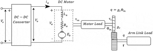
The mathematical equation representing the electrical and mechanical dynamics of a permanent magnet DC motor is given by Eq. (16(16) $V_a=R{i}_a+L\frac{d{i}_a}{dt}+K_b\frac{d{\theta }_m}{dt}$(16) ) (Spong & Vidyasagar, 2008).

(16) $V_a=R{i}_a+L\frac{d{i}_a}{dt}+K_b\frac{d{\theta }_m}{dt}$(16)

where, $V_a$ is the armature voltage of the motor, $R$ and $L$ are armature equivalent resistance and inductance, respectively. $K_b$is the back electromotive force constant, $i_a$ is the armature current, and ${\theta }_m$ denotes the angular position of motor.

Hence, the electromagnetic torque is due to the current through the armature winding and is proportional with this current. Mathematically, this can be written as:

(17) ${\tau }_m=K_m{i}_a$(17)

where,${\tau }_m$ is the generated motor torque, and $K_m$ is the diagonal matrix of the motor torque constant.

It ought to be noted that the application control input for driving the manipulator is the armature voltage of the dc motor. Therefore, by utilizing Eqs. (16)(16) $V_a=R{i}_a+L\frac{d{i}_a}{dt}+K_b\frac{d{\theta }_m}{dt}$(16) and (17(17) ${\tau }_m=K_m{i}_a$(17) ), and ignoring inductance$L$, due to its tiny amount (Sahin, 2005), the Eq. (18)(18) $\begin{array}{rl}& V_a=R{K_m}^{-1}[g_{r}M(q)+J_m{g_r}^{-1}]\ddot{q}+R{K}_m^{-1}[g_{r}B(q)(\dot{q},\dot{q})+g_{r}C(q)(\dot{q}{)}^2]+R{K}_m^{-1}[{\beta }_m{g_r}^{-1}\\ & +R^{-1}{K}_m{K}_b{g_r}^{-1}]\dot{q}+R{K}_m^{-1}{g}_{r}G(q)+R^{-1}{K}_m[g_{r}F(\dot{q})+g_r{\tau }_d]\end{array}$(18) is obtained.

(18) $\begin{array}{rl}& V_a=R{K_m}^{-1}[g_{r}M(q)+J_m{g_r}^{-1}]\ddot{q}+R{K}_m^{-1}[g_{r}B(q)(\dot{q},\dot{q})+g_{r}C(q)(\dot{q}{)}^2]+R{K}_m^{-1}[{\beta }_m{g_r}^{-1}\\ & +R^{-1}{K}_m{K}_b{g_r}^{-1}]\dot{q}+R{K}_m^{-1}{g}_{r}G(q)+R^{-1}{K}_m[g_{r}F(\dot{q})+g_r{\tau }_d]\end{array}$(18)

Finally, the complete nonlinear dynamic model representation of the 3-DOF robotic manipulator is given as:

(19) $\begin{array}{rl}& \left[\begin{array}{c}{\ddot{q}}_1\\ {\ddot{q}}_2\\ {\ddot{q}}_3\end{array}\right]={\left[\begin{array}{ccc}0.005r_1^2+0.029+0.035C_2^2+0.0067C_{23}^2+0.028C_2{C}_{23}& 0& 0\\ 0& 0.076+0.02778C_3& 0.0092+0.014C_3\\ 0& 0.017+0.02526C_3& 0.0707\end{array}\right]}^{-1}\left\{\left[\begin{array}{c}{V}_{a1}\\ V_{a2}\\ V_{a3}\end{array}\right]\right.\\ & -\left[\begin{array}{ccc}{b}_{11}& b_{12}& 0\\ 0& 0& b_{23}\\ 0& 0& 0\end{array}\right]\left[\begin{array}{c}{\dot{q}}_1\\ {\dot{q}}_1\\ {\dot{q}}_2\end{array}\begin{array}{c}{\dot{q}}_2\\ {\dot{q}}_3\\ {\dot{q}}_3\end{array}\right]-\left[\begin{array}{ccc}0& 0& 0\\ c_{22}& 0& c_{23}\\ c_{31}& c_{32}& 0\end{array}\right]\left[\begin{array}{c}{{\dot{q}}^2}_1\\ {{\dot{q}}^2}_2\\ {\dot{q}}_3^2\end{array}\right]\left.-\left[\begin{array}{c}0.25+2.66{\dot{q}}_1+0.04sgn({\dot{q}}_1)\\ 0.81C_2+0.272C_{23}+0.25+2.66{\dot{q}}_2+0.04sgn({\dot{q}}_2)\\ 0.248C_{23}+0.021+2.43{\dot{q}}_3+0.04sgn({\dot{q}}_3)\end{array}\right]\right\}\end{array}$(19)

3.4.2. Open loop system dynamic model description of the 3-DOF robotic manipulator

The open-loop dynamic model without using the controller was obtained using Matlab/Simulink as shown in Figure 4. To check the systems validity, fixed input voltages are selected for the manipulator’s joints, and afterward, the block is simulated.

Figure 4. Uncontrolled dynamic model Simulink diagram

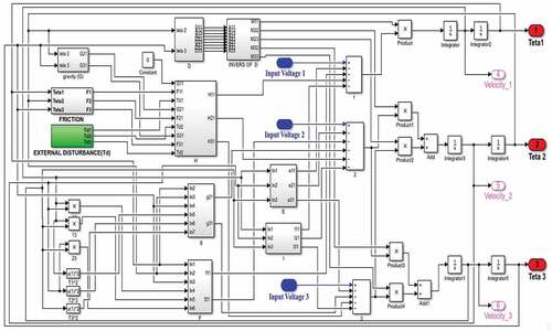
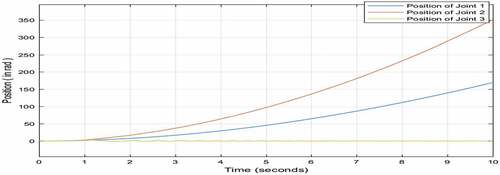
The open-loop uncontrolled dynamic model shows the impact of the input on the output state when a joint angle for computing input voltages U1, U2, and U3 for joints one, two, and three are utilized. Then the models simulation results are obtained for various input levels. Results in Figure 5 show that when all the input voltages of the manipulator are at an equilibrium or all three input voltages are at 0 v, then both the joints two and three are oscillated due to the gravitational impact of the earth. From the simulation results in Figures 5 and 6, it’s clear that the robot manipulator system is a highly coupled, nonlinear, and unstable system. Therefore, this has brought about the need to design a controller with an optimal performance.

Figure 5. Simulation of the open-loop dynamic model with U1 = U2 = U3 = 0 v

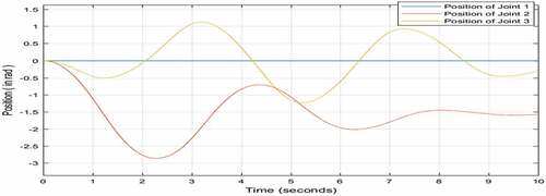
Figure 6. Simulation of the open-loop dynamic model with U1 = U2 = U3 = 12 v

4. ST-FSMC Controller design

Adaptation law plus FSMC can give a system capability of online-tuning and improve the systems trajectory tracking performance. The fuzzy adaptive technique can train the parameters variation by expert knowledge. Fuzzy adaptive method was used to solve the complicated uncertain nonlinear system (Darajat & Istiqphara, 2020), the integration of this adaptive method with the FSMC, therefore, helps the system to enhance its performance by online tuning of nonlinear and time-variant parameters (Jalali et al., 2013).

In a fuzzy controller, adaptation is divided into a direct adaptive technique and an indirect adaptive technique. The direct adaptive technique adjusts/tunes the controller inputs parameters, and an indirect supervisory technique adjusts/tunes the parameters of the control system depending on the performance error (Huang et al., 2018; Kim et al., 2020; Trigatti et al., 2018). A supervisory controller is a kind of adaptive controllers which searches to see the current performance of the system and adjusts the controller parameter to increase the systems performance.

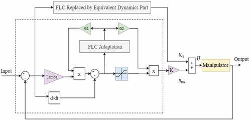
In this paper, a saturation function is utilized rather than a signum function in the discontinuous part of the SMC to eliminate the chattering effect on the control effort. Moreover, the adaptive fuzzy inference scheme is used to avoid perturbation. The ST-FSMC is proposed to discard the unstructured model uncertainty. Lamda (λ) and (K) are the coefficients having an important impact on the discontinuous part of the control system. In the proposed controller for the self-tuning part, these two significant gains are adjusted. Therefore, if these coefficients are tuned properly, the SMC can discard perturbations more desirably. Accordingly, Self-tuning-FSMC has powerful resistance and can solve uncertainty problems. The block diagram of the proposed self-tuning FSMC is presented in Figure 7.

Figure 7. Block diagram of adaptive (self-tuning) fuzzy sliding mode controller with fuzzy non-linear parts

To ensure that the system is asymptotically stable during the reaching phase, Lyapunov’s stability theorem was applied. Lyapunov-based method was utilized to obtain conditions of the sliding surface. It gives a positive scalar function called the Lyapunov candidate function presented in Eq. (21)(21) $V(s)=\frac{1}{2}{s}^2,V(s)=\frac{1}{2}{s}^2>0$(21) . For the system state variable, the control law that will diminish this function has been assumed as:

(20) $V>0$(20)

For picking the Lyapunov candidate function, there is no standard law. To investigate the stability of the system, the positive Lyapunov candidate function for each separate dynamic system best suitable function was chosen as follows:

(21) $V(s)=\frac{1}{2}{s}^2,V(s)=\frac{1}{2}{s}^2>0$(21)

(22) $\dot{V}(s)=s\dot{s}=s(-Ksign(s))=-\left|s\right|K<0,\dots \text{l}dots..if\dots \dots K>0$(22)

where, $s$and$\dot{s}$ are defined as a sliding function and its derivative, and $K$ is a design constant that must be higher than zero to meet the Lyapunov stability condition in the Eqs. (21)(21) $V(s)=\frac{1}{2}{s}^2,V(s)=\frac{1}{2}{s}^2>0$(21) and (22(22) $\dot{V}(s)=s\dot{s}=s(-Ksign(s))=-\left|s\right|K<0,\dots \text{l}dots..if\dots \dots K>0$(22) ).

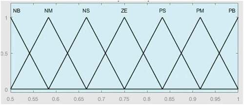
The FLC adjusts the system to different disturbances with one input, s and one output, α as shown in Figures 8 and 9. This Fuzzy Logic supervisor increases the trajectory tracking performance by online tuning of the controller parameters using the output, α, through the gain, G₁, and G₂. The scaled factors are: $G_1=0.9$, $G_2=10$ for the first joint; $G_1=1$, $G_2=5$ for the second joint, and $G_1=1$, $G_2=5$for the third joint.

Figure 8. Triangular membership function for input (s)

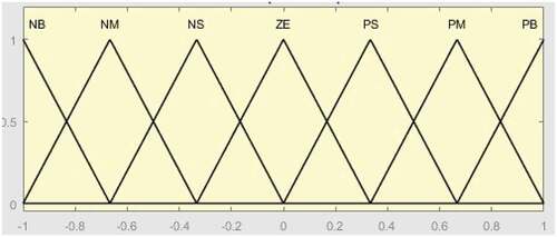
Figure 9. Triangular membership function for output (α)

5. Results and discussion

In this section, the performance and stability of the proposed control method were analyzed with and without uncertainty (external disturbance and parameter variation). The simulations were performed using MATLAB/Simulink. To confirm the performance of the proposed controller, the simulation results were compared with the conventional controllers.

For experimental purpose, the desired trajectory for the robotic manipulator is picked arbitrarily to check the tracking capability of the proposed controller (STFSMC) and other conventional controllers. Based on the results, ST-FSMC achieved a better performance than all other conventional controllers.

The robustness of the designed controller was also tested based on its power of disturbance elimination and sensitivity to parameter variation (mass uncertainty). This was also obtained for the conventional controllers. The value of disturbance applied to the desired trajectory of the joint variable was predefined. The mass term was considered as parameter variation. Based on the results, ST-FSMC was found to be more robust than PID, SMC, and FSMC.

5.1. Performance of proposed controller (ST-FSMC)

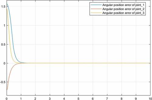
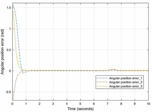
The response of ST-FSMC for the 3-DOF robot manipulator is shown in Figure 10 for angular position tracking error performance of joints one, two, and three respectively. Figure 10 shows that the tracking error converges to zero. In Table 3, the performance of the ST-FSMC angular position of joints with minimum time and without overshot as needed for the design of the ST-FSMC was presented. The results show that the end effector of the robot manipulator asymptotically follows the desired trajectory with minimum acceptable error. This indicates that the ST-FSMC control system is stable.

Figure 10. Angular position tracking error using ST-FSMC without disturbance and parameter variation

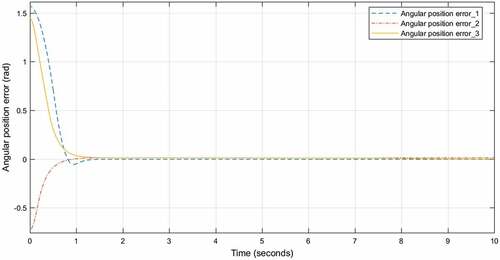
Table 3. Performance of the ST-FSMC angular position of joints

Performance	Angular position joint 1	Angular position joint 2	Angular position joint 3
Rising time(s)	0.4351	0.4283	0.3714
Settling time(s)	0.8261	0.8010	0.6906
Overshoot (%)	0	0	0
Steady state error	0.0008	0.0052	0.005
RMS error	0.4395	0.1603	0.3348
Chattering	Free	Free	Free
Average Steady state error (rad)	0.0037

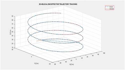
Figure 11 shows the trajectory tracking performance of the end-effector of the robot manipulator using ST-FSMC for 3D-helical trajectory. Figure 11 shows 3D-helical desired trajectory which is produced when the position of the end effector is starting initially from point $(100,0,15)cm$ following the trajectories$(70sin(t),50cos(t),15+3.5t)cm$ in the$X$, Y, and $Z$coordinates, respectively.

Figure 11. 3D-helical trajectory tracking using ST-FSMC

5.2. Performance comparison of proposed controller with other conventional controller without disturbance and parameter variation

The comparison of the designed controller (ST-FSMC, FSMC, SMC, and PID controller) for trajectory tracking performance is discussed as follows. Figure 12 shows the plot of the angular position tracking error using PID for joints one, two, and three. The results show that the steady-state error increased to 0.04 rad, 0.036 rad and 0.0476 rad (i.e., the average steady-state error was increased to 0.0413 rad), while the overshoot increased, rise time decreased by 0.1495 sec, 0.0975 sec, and 0.257sec, and settling time is increased by 5.56 sec, 0.69 sec, and 1.3 sec for joint one, two, and three respectively when the PID controller is used.

Figure 12. Angular position tracking errors using PID controller without disturbance and parameter variation

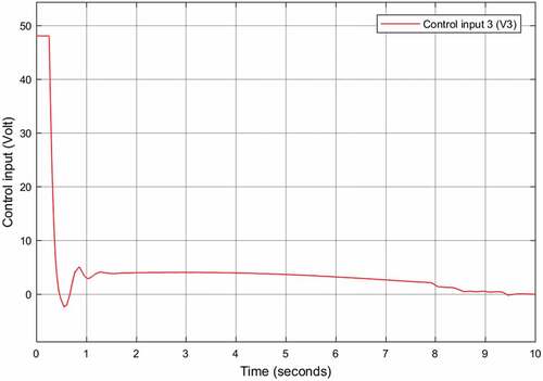
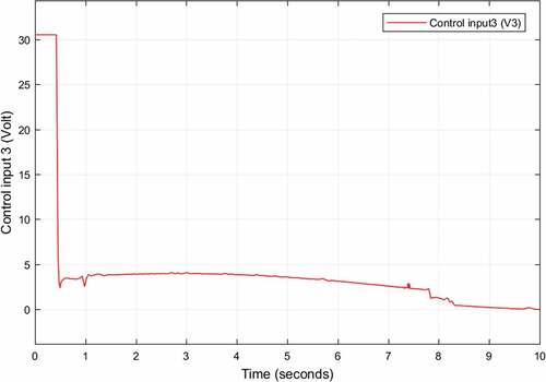
Figures 13, 14, and 15 show the control effort of joint one, joint two, and joint three of the PID controller, respectively. The results indicate that a very high control effort is needed to track the desired trajectory using PID relative to the proposed controller (ST-FSMC) control effort. The maximum voltage used to track the desired trajectory with PID needs 48 v for all three joints. This is increased by 23.5 v, 29 v, and 16.8 v for joint one, joint two, and joint three respectively.

Figure 13. Control effort of joint one using PID without disturbance and parameter variation

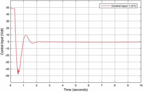
Figure 14. Control effort of joint two using PID without disturbance and parameter variation

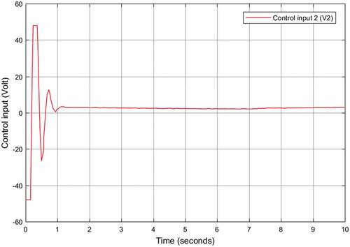
Figure 15. Control effort of joint three using PID without disturbance and parameter variation

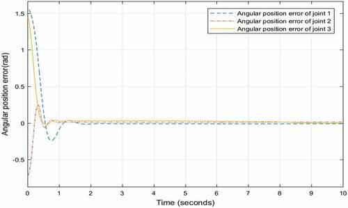
Figure 16 shows the plot of the angular position tracking error using pure SMC for joints one, two, and three respectively. Based on the results obtained, the performance of the pure SMC is almost the same as that of ST-FSMC for all three joints. The results show the performance of angular position of each joint in case of SMC with signum function (pure SMC) is also the same performance as compared to ST-FSMC, but it introduces high-frequency oscillation (chattering phenomena) on the control effort for tracking the desired trajectory. The chattering observed in the corresponding results with pure SMC is evident in the difficulty involved in the practical design of controller using this technique. This is one of its draw-backs.

Figure 16. Angular position tracking errors using SMC with signum function without disturbance and parameter variation

To overcome the problem of chattering in pure SMC, a saturation function was replaced in place of signum function. Figure 17 shows the plot of the angular position tracking error for joints one, two, and three. The results show that the steady-state error for SMC with boundary layer is 0.006 rad for joint one, 0.0032 rad for joint two, and 0.0036 rad for joint three (i.e., the average steady-state error increases to 0.0044), and the overshoot remains the same, while both the rise time and settling time were increased when SMC with saturation function was used.

Figure 17. Angular position tracking errors using SMC with boundary layer (sat function) without disturbance and parameter variation

We can conclude based on the simulation result that due to the replacement of the saturation function with signum function, the error performance increased against the considerable chattering elimination. Figures 18, 19, and 20 show the control effort of joints one, two, and three of SMC with saturation function respectively. The maximum voltage required to track the desired trajectory by SMC with saturation function is 25 v for joint one, 21.4 v for joint two, and 34.26 v for joint three. This is increased by 0.5 v, 2.4 v, and 3.06 v respectively compared to ST-FSMC.

Figure 18. Control effort of joint one using SMC with saturation function without disturbance and parameter variation

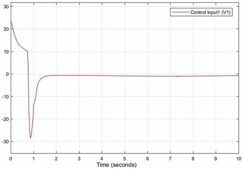
Figure 19. Control effort of joint two using SMC with saturation function without disturbance and parameter variation

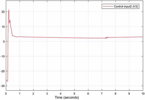
Figure 20. Control effort of joint three using SMC with saturation function without disturbance and parameter variation

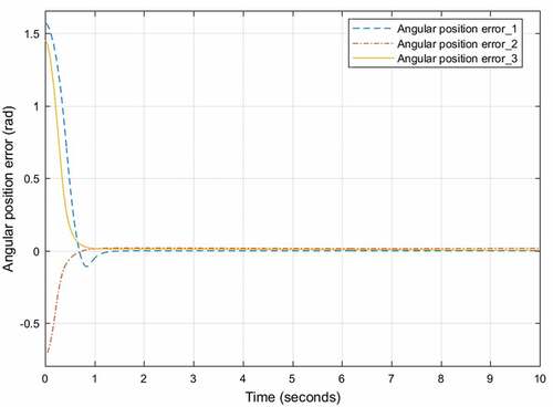
Figure 21 shows the results obtained for the angular position tracking error using FSMC. The simulation results show that the performance of FSMC is almost similar to that of SMC with saturation function in terms of overshoot size, rising and settling time, and steady-state error. The steady-state error of the joint one for the FSMC is 0.0052, it is 0.0065 for the SMC with saturation. The average steady-state error of three joints for the FSMC is 0.0053, for the SMC it is 0.0044 with saturation. Also the rising and settling time for the FSMC is almost similar to that of SMC with saturation function.

Figure 21. Angular position tracking errors using FSMC without disturbance and parameter variation

Figures 22, 23, and 24 show the control effort of joint one, two, and joint three of FSMC respectively. It requires high control effort relative to the ST-FSMC to track the desired trajectory. The maximum voltage used to track the desired trajectory by FSMC needs 25 v for joint one, 24.5 v for joint two, and 31.2 v for joint three. This increases by 0.6 v, 5.5 v, and 0 v respectively.

Figure 22. Control effort of joint three using FSMC without disturbance and parameter variation

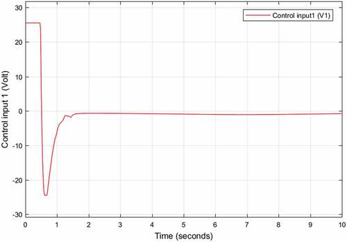
Figure 23. Control effort of joint three using FSMC without disturbance and parameter variation

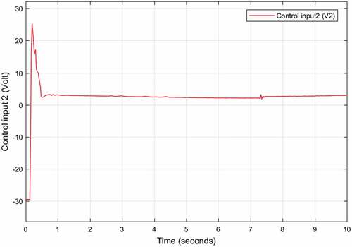
Figure 24. Control effort of joint three using FSMC without disturbance and parameter variation

According to the simulation result, the performance of ST-FSMC and pure SMC is better than FSMC, SMC with saturation function and PID controller for controlling robotic manipulators. The performance of the ST-FSMC was found to be superior to that of FSMC, SMC, and PID controllers with relatively low control effort required to track the desired trajectory.

5.3. Disturbance rejection and sensitivity to parameter variation of the controller

In the previous section, we showed the trajectory tracking performance without parameter variation and external disturbance in the system. In this section, the results with parameter variation and disturbance are presented and discussed.

5.3.1. Sensitivity to parameter variation of PID, SMC, FSMC, and ST-FSMC

In this section, the internal parameter variation (link parameter variation) is considered and then the performance of the ST-FSMC, FSMC, SMC, and PID is compared. For parameter variation, all the parameters are kept the same as presented in Table 2, except for $m_1$, $m_2,$and$m_3$which are changed to 2 kg each, that means considering an uncertainty in the value of the system to be controlled.

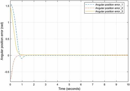
With reference to the simulation results obtained in Figures 25–28, we also compared the performance of the proposed controller with another conventional controller in the presence of structured uncertainty (link parameter variation). According to the simulation result, the performance of ST-FSMC results with parameter variation and without parameter variation is almost the same (i.e., rising time, settling time, overshoot, and steady-state error are approximately equal) relative to other controllers, while the average steady-state error for the three joints was increased by 0.0023. However, in the case of PID, SMC with the boundary layer, and FSMC controller, the system is highly affected by the parameter variation relative to ST-FSMC. For the PID controller with parameter variation, the rising time was increased by 0.05 sec, 0.06 sec, and 0.1 sec, while the settling time also increased by 1 sec, 1.3 sec, and 2.5 sec for joints one, two, and three respectively.

Figure 25. Angular position tracking errors using PID with parameter variation

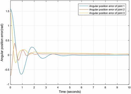
Figure 26. Angular position tracking errors using SMC with parameter variation

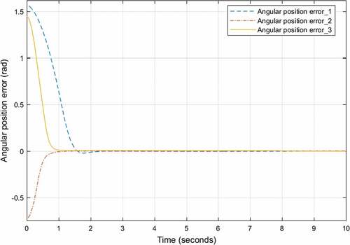
Figure 27. Angular position tracking errors using FSMC with parameter variation

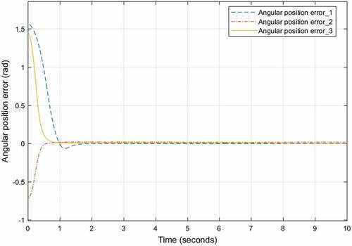
Figure 28. Angular position tracking errors using ST-FSMC with parameter variation

The average steady-state error for three joints is increased by 0.0427. For SMC with saturation function and parameter variation, the rising time was increased by 0.51 sec, 0.002 sec, and 0.0733 sec, while the settling time was increased by 1.02 sec, 0.02 sec, and 0.08 sec for joints one, two, and three respectively. The average steady-state error for the three joints was increased by 0.0336. For FSMC with parameter variation, the rising and setting time are almost the same as that of FSMC without parameter variation, but the overshoot increased, and also the average steady-state error for the three joints is increased by 0.0073.

5.3.2. Disturbance rejection capability of PID, SMC, FSMC, and ST-FSMC

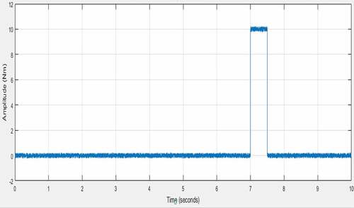
Robot manipulators are often tasked with working in environments with vibrations and are subject to load uncertainty. In this section, the proposed controllers are tested in terms of rejecting the uncertain disturbance torques caused by external vibration and payload variation. The Figures 29, 30, and 31 show the disturbance torques due to vibration, the disturbance torques due to payload variation effects, and the sum of disturbance torques due to vibration and payload variation respectively.

Figure 29. Disturbance torques due to vibration

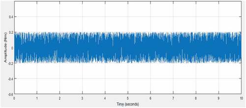
Figure 30. Disturbance torques due to payload variation effect

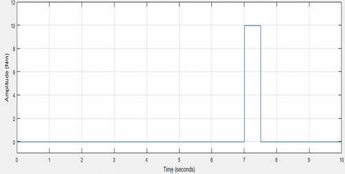
Figure 31. Disturbance torques due to vibration and payload variation combination

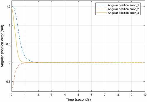
Figures 32, 33, 34, and 35 show the plot of angular position tracking errors for each joint using PID, SMC FSMC, and ST-FSMC respectively under uncertain external disturbances. The results show the performance of the angular position of each joint. ST-FSMC showed a high capability in handling the newly introduced uncertain external disturbance as compared to other conventional controllers as shown in Figure 35 of the angular position tracking error for joints one, two, and three using STFSMC under external disturbance. It’s clear that the results show that the designed controller (ST-FSMC) makes the system insensitive to parametric variations (it has good performance with variation in mass parameters). It is also robust and performs well even in the presence of external disturbances with minimum tracking error as compared to PID, SMC, and FSMC controllers with considerable control effort. Generally from the results, the ST-FSMC is more robust than the FSMC, SMC, and PID controller.

Figure 32. Angular position tracking errors using PID under uncertain external disturbance

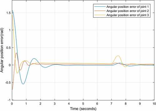
Figure 33. Angular position tracking errors using SMC under uncertain external disturbance

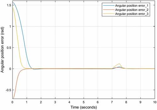
Figure 34. Angular position tracking errors using FSMC under uncertain external disturbance

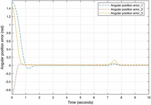
Figure 35. Angular position tracking errors using ST-FSMC under uncertain external disturbance

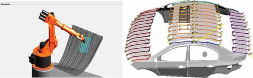
5.4. Application of robot manipulators in 3-D industrial target task

5.4.1. Robot manipulator for painting and welding in automation industry

One of the tasks performed in a vehicle automation industry is painting and welding the upper part of the vehicles body. The trajectory tracking performance of a robot manipulator was discussed in the previous sections of this paper utilizing the proposed control system with a 3D-helical trajectory as the desired trajectory and various conventional controllers. The trajectory planning of the 3-DOF robot manipulator in welding and painting the vehicles body was explored in this section to improve the quality of painting and welding in the automobile industry. In summary, the advancement of robotized welding and painting is very remarkable, and is now one of the most important aspects of the automobile industry. Because of these advantages for humans, it is excellent for use in the automotive industry to improve both painting and welding operations. As shown in Figure 36, the 3D-square wave trajectory was used as the desired trajectory for welding and painting of vehicles body.

Figure 36. 3D-square wave trajectory of the manipulator for welding and painting of vehicles body

The trajectory tracking performance of the 3D-square wave trajectory is shown in Figures 37 and 38. The actual trajectory is compared with the desired trajectory using PID, SMC, FSMC, and the proposed ST-FSMC controllers. Integral square error (ISE), integral absolute error (IAE), integral time square error (ITSE), and integral time absolute error (ITAE) indices were used as performance measures. The results are summarized in the Tables 4, 5, 6 and 7.

Figure 37. 3D-square wave trajectory planning of the 3-DOF robot manipulator for welding and painting of vehicles body

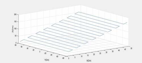
Figure 38. Trajectory tracking control of the 3-DOF robot manipulator

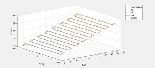
Table 4. Performance Index for PID controller

Trajectory Dynamics	ISE	IAE	ITSE	ITAE
X-axis	1.073	0.512	0.08145	0.09059
Y-axis	3.089	0.8813	0.2428	0.1614
Z-axis	0.3796	0.2866	0.02333	0.09409

Table 5. Performance Index for SMC controller

Trajectory Dynamics	ISE	IAE	ITSE	ITAE
X-axis	0.4223	0.1854	0.01181	0.008821
Y-axis	0.4672	0.336	0.03469	0.06729
Z-axis	0.1693	0.1605	0.02211	0.9636

Table 6. Performance Index for FSMC controller

Trajectory Dynamics	ISE	IAE	ITSE	ITAE
X-axis	1.798*10^−1	0.01295	8.721*10^−1	0.06423
Y-axis	0.1796	0.1866	0.004333	0.0019409
Z-axis	5.429*10^−1	0.006993	0.0002874	0.03558

Table 7. Performance Index for ST-FSMC Controller

Trajectory Dynamics	ISE	IAE	ITSE	ITAE
X-axis	3.69*10^−2	0.001133	1.829*10^−1	0.00513
Y-axis	0.01251	0.1020	0.001016	0.000258
Z-axis	8.438*10^−2	0.005329	1.376*10^−1	0.02348

The performance indices shown in Tables 4–7 show that a smaller error is obtained by ST-FSMC than when PID, SMC, and FSMC controllers were used in welding and painting the vehicles body. Finally, it can be said that the proposed controller for the 3-DOF robot manipulator control has a good performance and good transient response when excited with both 3-D helical and 3-D square wave trajectories.

6. Conclusion

In this paper, a self-tuning fuzzy sliding mode controller (ST-FSMC) was proposed. The ST-FSMC, PID, SMC, and FSMC were successfully designed and comparative analysis was carried out. Simulations were performed to demonstrate that the ST-FSMC is more effective in terms of the response time performance than other conventional controllers (PID, SMC, and FSMC) for a given desired trajectory tracking because the proposed controller can adjust itself to the system parameter’s variations and external disturbances. The simulation results further show the high ST-FSMC tracking performance and ability of the system to solve the problem of handling unstructured uncertainties and achieve stability, robustness as well as reliability. The stability of the designed controller was verified using Lyapunov`s Direct Method. Also, various evaluation criteria were chosen to compare the performance of the controller designed (ST-FSMC) with other controllers such as PID, SMC, and FSMC. The system performance in both SMC and FSMC were observed to have difficulty in handling uncertain external disturbances (unstructured uncertainties) because the sliding surface gain was chosen by trial and error, which means that the SMC and FSMC must have prior knowledge of the system uncertainty. In order to solve the problem of handling unstructured uncertainties to increase the robustness of the system and give an improved output, FSMC and Fuzzy base tuning controller methods were combined. This control method was implemented in the robotic manipulator to give a high-performance nonlinear controller in the presence of uncertainties. This paper assumed that the working environment of the system is clean (i.e., no obstacles around the working environment). Therefore, 3-DOF was used for reducing redundancy to perform a given task cyclically. In future works, authors intend to extend the system to better degree of freedom by considering the presence of obstacles to execute various tasks in different working environments by applying the same or any other control methodology addressed in this research work. Redundant manipulators are extensively used because of their ability to perform a prescribed end-effector motion (tracking problem), while taking into account extra goals such as obstacle avoidance or the minimization of energy consumption, or other cost functions. This is particularly important for manufacturing tasks, which often require robots to perform a repetitive task while keeping energy and time requirements as low as possible.

Additional information

Funding

The authors received no direct funding for this research.

Notes on contributors

Aderajew Ashagrie

Aderajew Ashagrie received a BSc. in Electrical and Computer Engineering from Arba Minch University and M.Sc. in Electrical and Computer Engineering (Industrial Control and Instrumentation Engineering) from Addis Ababa Science and Technology University, Ethiopia. He is currently working as a lecturer at Arba Minch University.

Ayodeji Olalekan Salau

Dr. Ayodeji Olalekan Salau received a B.Eng. in Electrical/Computer Engineering from the Federal University of Technology, Minna, Nigeria. He received an M.Sc. and Ph.D. degree in Electronic and Electrical Engineering from the Obafemi Awolowo University, Ile-Ife, Nigeria. In 2020, Dr. Salau’s paper was awarded the best paper of the year 2019 in Cogent Engineering. He is currently working at Afe Babalola University in the Department of Electrical/Electronics and Computer Engineering.

Tilahun Weldcherkos

Tilahun Weldcherkos received a BSc. in Electrical and Computer Engineering from Arba Minch University, and MSc. in Industrial Control and Instrumentation Engineering from Addis Ababa Science and Technology University, Ethiopia. He is currently working as a lecturer in Arba Minch University.

References

- Abbas, Z. (2018). Motion control of robotic arm manipulator using pid and sliding mode technique. PhD thesis. Capital University.
- Alassar, A. Z., Abuhadrous, I. M., & Elaydi, H. A. (2010). Comparison between FLC and PID controller for 5DOF robot arm. 2nd IEEE International Conference on Advanced Computer Control, 5, 277–33. Shenyang, China.
- Anh, H. P. H., Kien, C. V., Son, N. N., & Nam, N. T. (2018). New approach of sliding mode control for nonlinear uncertain pneumatic artificial muscle manipulator enhanced with adaptive fuzzy estimator. International Journal of Advanced Robotic Systems, 1–11. https://doi.org/10.1177/1729881418773204
- Bittencourt, A. C. (2007). Friction change detection in industrial robot arms. MSc Thesis KTH Electrical Engineering and Computer Science, Sweden, 1-79.
- Chang, Y., Yen, H., & Wu, H. (2008). An intelligent robust tracking control for electrically-driven robot systems. International Journal of Systems Science, 39(5), 497–511. https://doi.org/10.1080/00207720701832747
- Craig, J. J. (2009). Introduction to robotics: Mechanics and control, E. Pearson Education India.
- Darajat, A. U., & Istiqphara, S. (2020). Control of two-link robot manipulator with uncertainty parameter using self-tuning sliding mode control. 3rd International Conference on Mechanical, Electronics, Computer, and Industrial Technology (MECnIT), Medan, Indonesia. https://doi.org/10.1109/mecnit48290.2020.9166643
- Dhyani, A., Panda, M. K., & Jha, B. (2020). Design of an evolving fuzzy-PID controller for optimal trajectory control of a 7-DOF redundant manipulator with prioritized sub-tasks. Expert Systems with Applications, 162, 113021. https://doi.org/10.1016/j.eswa.2019.113021
- Fateh, M. M. (2008). On the voltage-based control of robot manipulators. International Journal of Control, Automation, and Systems, 6(5), 702–712. https://doi.org/10.1007/s12555-017-0035-0
- Gambhire, S. J., Kishore, D. R., Londhe, P. S., & Pawar, S. N. (2021). Review of sliding mode based control techniques for control system applications. International Journal of Dynamics and Control, 9(1), 363–378. https://doi.org/10.1007/s40435-020-00638-7
- Getachew, D. (2018). Sliding mode control of a two degree of freedom robot arm using permanent magnet synchronous motor. http://localhost:80/xmlui/handle/123456789/12687
- Ghaleb, N. M., & Aly, A. A. (2018). Modeling and control of 2-DOF robot arm. International Journal of Emerging Engineering Research and Technology, 6(11), 24–31. https://www.ijeert.org/papers/v6-i11/3.pdf
- Hu, H., & Woo, P. (2006). Fuzzy supervisory sliding-mode and neural network control for robotic manipulators. IEEE Transactions on Industrial Electronics, 53(3), 929–940. https://doi.org/10.1109/TIE.2006.874261
- Huang, J., Hu, P., Wu, K., & Zeng, M. (2018). Optimal time-jerk trajectory planning for industrial robots. Mechanism and Machine Theory, 121, 530–544. https://doi.org/10.1016/j.mechmachtheory.2017.11.006
- Jalali, A., Piltan, F., Gavahian, A., Jalali, M., & Adibi, M. (2013). Model-free adaptive fuzzy sliding mode controller optimized by particle swarm for robot manipulator. International Journal of Information Engineering and Electronic Business, 5(1), 68. https://doi.org/10.5815/ijieeb.2013.01.08
- Kapoor, N., & Ohri, J. (2013). Fuzzy sliding mode controller (FSMC) with global stabilization and saturation function for tracking control of a robotic manipulator. Journal of Control and Systems Engineering, 1(2), 50. https://doi.org/10.18005/JCSE0102003
- Kapoor, N., & Ohri, J. (2017). Sliding Mode Control (SMC) of robot manipulator via intelligent controllers. Journal of the Institution of Engineers (India): Series B, 98(1), 83–98. https://doi.org/10.1007/s40031-016-0216-x
- Karamali Ravandi, A., Khanmirza, E., & Daneshjou, K. (2018). Hybrid force/position control of robotic arms manipulating in uncertain environments based on adaptive fuzzy sliding mode control. Applied Soft Computing, 70, 864–874. https://doi.org/10.1016/j.asoc.2018.05.048
- Kim, J., Jin, M., Park, S. H., Chung, S. Y., & Hwang, M. J. (2020). Task space trajectory planning for robot manipulators to follow 3-d curved contours. Electronics, 9(9), 1424. https://doi.org/10.3390/electronics9091424
- Korayem, M. H., Alamdari, A., Haghighi, R., & Korayem, A. H. (2010). Determining maximum load-carrying capacity of robots using adaptive robust neural controller. Robotica, 28(7), 1083. https://doi.org/10.1017/S0263574710000081
- Marton, L., & Lantos, B. (2007). Modeling, identification, and compensation of stick-slip friction. IEEE Transactions on Industrial Electronics, 54(1), 511–521. https://doi.org/10.1109/TIE.2006.888804
- Massaoudi, F., Elleuch, D., & Damak, T. (2019). Robust control for a two DOF robot manipulator. Journal of Electrical and Computer Engineering, 2019, 1–11. https://doi.org/10.1155/2019/3919864
- Medhaar, H., Derbel, N., & Damak, T. (2006). A decoupled fuzzy indirect adaptive sliding mode controller with application to robot manipulator. International Journal of Modelling, Identification and Control, 1(1), 23–29. https://doi.org/10.1504/IJMIC.2006.008644
- Ohri, J., Vyas, D. R., & Topno, P. N. (2011). Comparison of robustness of PID control and sliding mode control of robotic manipulator. International Symposium on Devices MEMS Intelligent Systems and Communication (ISDMISC), Bhopal, India, 5–10.
- Pezeshki, S., Badalkhani, S., & Javadi, A. (2012). Performance analysis of a neuro-pid controller applied to a robot manipulator. International Journal of Advanced Robotic Systems, 9(5), 163. https://doi.org/10.5772/51280
- Piltan, F., Yarmahmoudi, M. H., Shamsodini, M., Mazlomian, E., and Hosainpour, A. (2012a). PUMA-560 robot manipulator position computed torque control methods using Matlab/Simulink and their integration into graduate nonlinear control and Matlab courses. International Journal of Robotics and Automation, 3(3), 167–191
- Piltan, F., Rahmdel, S., Mehrara, S., and Bayat, R. (2012b). Sliding mode methodology vs. Computed torque methodology using matlab/simulink and their integration into graduate nonlinear control courses. International Journal of Engineering, 6(3), 142–177. https://www.cscjournals.org/manuscript/Journals/IJE/Volume6/Issue3/IJE-369.pdf
- Rahmdel, S., Bairamai, M., & Fahham, M. M. H. R. (2012). Design chattering-free performance-based fuzzy sliding mode controller for bus suspension. International Journal of Engineering Sciences Research (IJESR), 796–802.
- Sahin, H. (2005). Design of a secondary packaging robotic system. PhD Graduate School of Natural and Applied Sciences of Middle East Technical University, p. 156.
- Shaei, S. E. (2010). Sliding mode control of robot manipulators via intelligent approaches. Citeseer.
- Spong, M. W., & Vidyasagar, M. (2008). Robot dynamics and control. John Wiley & Sons, 2008, 352.
- Tao, C. M., & Lee, T. (2016). Adaptive fuzzy sliding mode controller for linear systems with mismatched time-varying uncertainties. 59th IEEE International Midwest Symposium on Circuits and Systems (MWSCAS), 283–294.
- Trigatti, G., Boscariol, P., Scalera, L., Pillan, D., & Gasparetto, A. (2018). A look-ahead trajectory planning algorithm for spray painting robots with non-spherical wrists. IFToMM symposium on mechanism design for robotics, 235–242.
- Wai, R. (2003). Tracking control based on neural network strategy for robot manipulator. Neurocomputing, 51, 425–445. https://doi.org/10.1016/S0925-2312(02)00626-4
- Wang, Y., Shi, R., & Wang, H. (2014). ESO-based fuzzy sliding-mode control for a 3-DOF serial-parallel hybrid humanoid arm. Journal of Control Science and Engineering, 1–9. https://doi.org/10.1155/2014/304590
- Yin, H., Li, Y., & Li, J. (2017). Decomposed dynamic control for a flexible robotic arm in consideration of nonlinearity and the effect of gravity. Advances in Mechanical Engineering, 9(2), 168781401769410. https://doi.org/10.1177/1687814017694104
- Zhang, H., Fang, H., Zhang, D., Luo, X., & Zou, Q. (2020). Adaptive fuzzy sliding mode control for a 3-DOF parallel manipulator with parameters uncertainties. Complexity, 2565316, 16. https://doi.org/10.1155/2020/2565316