A non-Secant quasi-Newton Method for Unconstrained Nonlinear Optimization

Abstract

The Secant equation has long been the foundation of quasi-Newton methods, as updated Hessian approximations satisfy the equation with each iteration. Several publications have lately focused on modified versions of the Secant relation, with promising results. This study builds on that idea by deriving a Secant-like modification that uses non-linear quantities to construct Hessian (or its inverse) approximation updates. The method uses data from the two most recent iterations to provide an alternative to the Secant equation with the goal of producing improved Hessian approximations that induce faster convergence to the objective function optimal solution. The reported results provide strong evidence that the proposed method is promising and warrants further investigation.

Keywords:

• quasi-Newton methods
• Secant-like methods
• BFGS
• unconstrained optimization
• multi-step methods

Public interest statement

Unconstrained optimization problems are common in industrial and engineering applications. Much research has been dedicated to devise efficient methods to solve such problems. Secant Quasi-Newton methods constitute the basis for such methods due to their attractive properties. This paper derives a new nonlinear variant of the classical Secant methods that efficiently computes solutions to unconstrained optimization problems.

1. Introduction

The techniques examined in this paper are those employed in the solution of problems of the form

$minf\left(x\right){,}_{}wheref:R^n\to R.$

Such issues are common in all types of engineering and manufacturing projects. The above problem is solved iteratively using quasi-Newton methods. For the current iteration i, the gradient of f at $x_i$ is indicated as $g_i$ and the matrix $B_i$ is approximates $G(x_i)$, the actual Hessian of f. The next iteration Hessian matrix approximation must traditionally satisfy the so-called Secant equation

(1) $B_{i+1}{s}_i=y_i,$(1)

for

$y_i=g_{i+1}-g_i$ and $s_i=x_{i+1}-x_i$.

The new solution approximation is defined as

(2) $x_{i+1}=x_i+{\alpha }_i{p}_i,$(2)

where $p_i$ the direction vector, obtained through solving

(3) $B_i{p}_i=-g_{i}or{p}_i=-H_i{g}_i.$(3)

The step length ${\alpha }_i$ in (2) is computed as the solution to

${\alpha }_i={\hspace{0.17em}}_{\alpha \in R^{+}}^{min}f\left(x_i+\alpha p_i\right),$

by means of some line search methodology to satisfy conditions the following Wolfe-Powell- conditions are satisfied (Fletcher (1987))

(4) $f\left(x_{i+1}\right)\le f\left(x_i\right)+{10}^{-4}{s}_i^T{g}_i$(4)

and

(5) $s_i^T{g}_{i+1}\ge 0.9p_i^T{g}_i.$(5)

Satisfying conditions of the type in (4) and (5) is necessary to guarantee convergence.

The derivation and coding of the actual Hessian matrix is susceptible to human error and demands considerable storage for large problems. The identity matrix (or some weighted version of it) is usually chosen as the initial approximation to the Hessian, and it is updated step-by-step using the most recent available computed data. It has been demonstrated that such methods exhibit superlinear convergence under reasonable assumptions about the objective functions (Fletcher, 1970, 1994; Dennis & Schnabel, 1979). When the line searches are exact, the methods converge in at most n iterations on quadratic functions (Broyden, 1970).

The most numerically successful update formula used to approximate the Hessian on a step-wise basis is the BFGS update and is given as

$B_{i+1}^{\hspace{0.17em}}=B_i+\frac{y_i{y}_i^T}{s_i^T{y}_i}-\frac{B_i{s}_i{s}_i^T{B}_i}{s_i^T{B}_i{s}_i}.$

The global convergence of the BFGS method for convex objective functions has been established by some authors (see, Dai et al., 2002; Dennis & Schnabel, 1979; Fletcher, 1987; Shanno, 1978; Shanno & Phua, 1978; Xiao et al., 2006; Yuan et al., 2018, 2017). Dai et al. (2002) demonstrate that when the line searches are inexact, the standard BFGS method may fail to converge on non-convex functions. Wei et al. (2004, 2006) show that even with accurate-line searches, the classical BFGS method can fail to converge. Li and Fukushima (2001) modified the classical BFGS formula to create a variant of the method that exhibits global convergence even when the objective function f lacks the convexity condition.

2. Variants of the Secant equation

Much research has been conducted in order to develop methods that outperform the classical BFGS update numerically and are globally convergent under reasonable assumptions. In this section, we provide a brief overview of some of the successful methods that have outperformed the classical BFGS. The algorithms’ development is primarily based on the introduction of modifications to the Secant equation (1)(1) $B_{i+1}{s}_i=y_i,$(1) . The concept of using more of the data available at each iteration in the update of the Hessian approximation that would otherwise be disregarded motivates one particularly successful class of approaches documented in the literature. These data include, though not limited to, the readily computed step vectors as well as the gradient difference vectors in (1) from the m latest iterations (m > 1). The standard quasi-Newton methods utilize just from the most recent iteration. We next present a particularly successful class of methods known as the multi-step methods (Ford & Moghrabi, 1993, 1994, 1996).

Applying the Chain Rule is applied to g $\left(\mathrm{x}\left(\tau \right)\right)$, for a differentiable path in $R^n$, $X=\left\{x\left(\tau \right)\right\}$ (for $\tau \in R)$, and differentiate with respect to $\tau$, the result is

(6) $G\left(x_{i+1}\right)x{ }^{\mathrm{\prime }}\left({\tau }_m\right)=g{ }^{\mathrm{\prime }}\left(x\left({\tau }_m\right)\right).$(6)

In particular, if m is chosen to pass through the most recent point $x_{i+1}$ (so that $x\left({\tau }_m\right)=x_{i+1}$, say), then equation (6)(6) $G\left(x_{i+1}\right)x{ }^{\mathrm{\prime }}\left({\tau }_m\right)=g{ }^{\mathrm{\prime }}\left(x\left({\tau }_m\right)\right).$(6) , known as the “Newton Equation” (see, Al-Baali, 1985; Broyden, 1970; Dennis & Schnabel, 1979), presents generally an alternative that the Hessian matrix $G\left(x_{i+1}\right)$ satisfies. Equation (6)(6) $G\left(x_{i+1}\right)x{ }^{\mathrm{\prime }}\left({\tau }_m\right)=g{ }^{\mathrm{\prime }}\left(x\left({\tau }_m\right)\right).$(6) may be regarded as a basis for the Secant equation when m is chosen to be i + 1 (Broyden, 1970). In Ford and Moghrabi (1994), the path $X$ is constructed as the polynomial interpoloating the $m+1$ most recent points $\{x_{i-m+k+1}{\}}_{k=0}^m$. The polynomial ($\hat{g}\left(\tau \right)$, say) is used to approximate the vector $g{ }^{\mathrm{\prime }}\left(x\left({\tau }_m\right)\right)$ that by differentiating the corresponding polynomial which interpolates the corresponding available gradient points $\{g\left(x_{i-m+k+1}\right){\}}_{k=0}^m$.

The scalar values $\{{\tau }_k{\}}_{k=0}^m$ correspond to the points $\{x_{i-m+k+1}{\}}_{k=0}^m$ on the curve $X=\left\{x\left(\tau \right)\right\}$ as follows

$x\left({\tau }_k\right)=x_{i-m+k+1},\hspace{0.17em}for\hspace{0.17em}k=0,1,\dots ,m.)$

If $B_{i+1}$ is a given approximation to $G\left(x_{i+1}\right)$ in (6) and we make the following definitions

(7) $\underset{i\to \mathrm{\infty }}{lim}{f}_i=f^{\ast }.$(7)

(8) $l_{1}p{ }^2\le d^T{\mathrm{\nabla }}^{2}f\left(x\right)d\le l_{2}p{ }^2$(8)

(where the vectors $s_i$ and $y_i$ are as defined in (1) and $w_i$ represents an approximation to $g{ }^{\mathrm{\prime }}\left(x\left({\tau }_m\right)\right)$, it is not ureasonable (by (6)) to force the matrix $B_{i+1}$ to satisfy a relation similar to the one in (6). We, thus, have

(9) $B_{i+1}{r}_i=w_i.$(9)

There remains the issue of choosing values for the τ parameters. One possibile choice is (Ford & Moghrabi, 1993)

(10) ${\tau }_0=-\left(||{s_i}_2||+||{s_{i-1}}_2||\right),{\tau }_2=0,\mathrm{a}\mathrm{n}\mathrm{d}{\tau }_1=-||{s_i}_2||.$(10)

This choice has the merit of reflecting the distances among the iterates in the space of the variables and updated for each new point.

The multi-step BFGS Hessian update is given by

(11) $B_{i+1}^{MS}=B_i+\frac{w_i{w}_i^T}{w_i^T{r}_i}-\frac{B_i{r}_i{r}_i^T{B}_i}{r_i^T{B}_i{r}_i}.$(11)

The main advantage of (10) is in exploiting several recent steps as well as available gradient vectors in contrast to the standard BFGS method that utilizes only latest one-step and the corresponding gradient difference vectors.

Other non-secant methods are motivated by the fact that the classical BFGS formula is confined to using single gradient and step vectors in the construction of the Hessian approximation while neglecting other potentially useful readily computed data. For example, function values might prove to be valuable in the updating process. So, focusing on building better ‘quality’ updates, variants of the classical Secant relation (1) have been explored (see, Ford & Moghrabi, 1996; Wei et al., 2004; Ortiz et al., 2004; G. Yuan & Wei, 2010; Yuan et al., 2010, 2017, 2018; Zhang et al., 1999). Wei et al. (2006), using Taylor’s series, derived a modification to (1) as follows:

$B_{i+1}{s}_i=z_i,$

where, $z_i=y_i+\frac{{\theta }_i}{||{s_i}^2||}$ and ${\theta }_i=2\left(f_i-f_{i+1}\right)+{\left(g_{i+1}+g_i\right)}^T{s}_i.$

G. Yuan and Wei (2010) used another alternative, given as:

$z_i=y_i+\frac{\mathrm{m}\mathrm{a}\mathrm{x}\left(0,{\theta }_i\right)}{||{s_i}^2||}.$

Some of the recent and well-known Secant-like methods that are motivated by the need to derive accelerated convergence variants of the classical BFGS may be summarized in Table 1.

Table 1. Some modifications of Secant equation

Author(s)	The derived Secant variant	Ref.
Fletcher	$B_{i+1}{s}_i={\vartheta }_i{y}_i+\left(1-{\vartheta }_i\right)B_i{s}_i$	Fletcher (1987)
Zhang et al.	$B_{i+1}{s}_i=y_i+\frac{6\left(f_i-f_{i+1}\right)+3{\left(g_{i+1}+g_i\right)}^T{s}_i}{s_i^T{s}_i}{s}_i$	Zhang et al. (1999)
Wei et al.	$B_{i+1}{s}_i=y_i+\frac{2\left(f_i-f_{i+1}\right)+{\left(g_{i+1}+g_i\right)}^T{s}_i}{s_i^T{s}_i}{s}_i$	Wei et al. (2006)
Li and Fukushima	$B_{i+1}{s}_i=y_i+{\sigma }_i{s}_i$, ${\sigma }_i<{10}^{-6}$	Li and Fukushima (2001)
Yuan et al.	$B_{i+1}{s}_i=y_i$$+\frac{\mathrm{m}\mathrm{a}\mathrm{x}\left(0,2\left(f_i-f_{i+1}\right)+{\left(g_{i+1}+g_i\right)}^T{s}_i\right)}{s_i^T{s}_i}{s}_i$	Yuan et al. (2017)
Hassan	$B_{i+1}{s}_i=\frac{1}{2}{y}_i+\frac{\left(f_i-f_{i+1}\right)-0.5{g_{i+1}}^T{s}_i}{s_i^T{y}_i}{y}_i$	Hassan (2020)
Hassan and Mohammed	$B_{i+1}{s}_i=y_i-\frac{{g_{i+1}}^T{s}_i}{s_i^T{y}_i}{y}_i$	Hassan and Mohammed (2020)
Hassan and Ghada	$B_{i+1}{s}_i=y_i+\frac{2\left(f_i-f_{i+1}\right)-{y_i}^T{s}_i}{s_i^T{y}_i}{y}_i$	Hassan and Ghada (2020)

Although the methods listed in Table 1 represent some of the well-known published Secant-variant formulae that in addition to incorporating gradient and step vectors function values obtained from the latest iterate are exploited in the update of the Hessian approximation. To differ, the methods derived in Moghrabi (2017) and Ford and Moghrabi (1993), utilize nonlinear interpolating polynomials, and introduce a completely different Secant-like equation utilizing available data from the two/three most recent steps. The methods of Moghrabi (2017) are based on the idea of performing multiple updates on each iteration so that multiple Secant and Secant-variant conditions are observed. The updates are performed in a manner that ensures the first update obeys (1) while subsequent updates satisfy

$B_{i+1}^{\left(t+1\right)}{v}^t=u^t,t=1,2,m-1\left(m>1\right)$

where $v^t=r_{i-m+t}$ and $u^t=w_{i-m+t}$, for r and w as in (7) and (8).

A sample of the work done on the derivation of modified Secant equations is summarized in Table 1. For interested readers, there are many other similar methods available in the literature (Wei et al., 2006; Xiao et al., 2006; Yuan et al., 2018; G. Yuan & Wei, 2010; Yuan et al., 2017, 2010; Zhang et al., 1999). Several of the approaches mentioned here have had their convergence qualities investigated. Yuan et al. (2018), for example, demonstrate global convergence using a less stringent variant of the Powell-Wolfe line search criteria (4) and (5).

Such methods may prove useful in various domains in which the classical BFGS has been a serious contender. One possible domain is in sustainable transportation planning for dealing with the issue of minimizing air pollution, congestion, and noise (Sayyadi & Awasthi, 2018). Another possible application could be in the bi-objective inventory model created by Gharaei et al. (2020). The goal of to optimize the lot-sizing of the replenishment while meeting stochastic limitations and calculating the optimal number of lots and volume of each lot. Gharaei et al. (2015) aim to optimize incentives in single machine scheduling in reward-driven systems such that total reward is maximized while limitations such as total reward limitation for earliness and learning, independence from earliness and learning, and others are met. The goal is to maximize overall rewards in the mentioned system by using quadratic rewards for both learning and earliness, where non-secant methods may prove useful. Gharaei et al. (2019) present a mathematical model that combines the buyers’ and vendors’ total costs (TC) in a supply chain (TC) under penalty, green, and quality assurance (QC) rules, as well as a VMI-CS agreement. The goal is to find the optimal batch-sizing policy in the integrated SC with the lowest TC that finds both the number of the vendor’s batches for each of the shipped product lines and the size of the batches shipped to the buyers in order to minimize the integrated SC’s TC while satisfying the stochastic barriers. Due to the complexity of the optimization model, the possibility of employing the methods proposed in this paper for solving the integrated supply chain problem. Another attractive application might be in areas where quality control and green production policies are considered when designing a bi-objective multi-product limited and integrated economic production quantity model. There are stochastic constraints in the model mentioned above. Such research aims to find the best total inventory cost and total profit while keeping stochastic restrictions in mind (see, Gharaei et al. (2021)). Awasthi & Omrani, (2019) propose a goal-oriented strategy for prioritizing sustainable mobility projects based on fuzzy axiomatic design. The affinity diagram technique is used to establish sustainability evaluation attributes. The criteria and alternatives are rated using the fuzzy Delphi technique. Fuzzy axiomatic design provides final rankings for urban transportation initiatives, and the best project(s) are picked for implementation. Sensitivity analysis is used to examine the impact of changes in input parameters on the model’s stability, and this is a possible venue for the method proposed in this paper to prove its usefulness.

Next a new method that is motivated by the same concept of incorporating data available from several of the latest iterations for deriving a new variant to the Secant equation (1)(1) $B_{i+1}{s}_i=y_i,$(1) is developed.

3. A New Non-Secant equation

We will use data from three most recent iterations to derive the new Secant-like relationship that the updated Hessian (or its inverse) must fulfil, just as we did with the nonlinear multi-step quasi-Newton methods (equations (5(5) $s_i^T{g}_{i+1}\ge 0.9p_i^T{g}_i.$(5) –10(10) ${\tau }_0=-\left(||{s_i}_2||+||{s_{i-1}}_2||\right),{\tau }_2=0,\mathrm{a}\mathrm{n}\mathrm{d}{\tau }_1=-||{s_i}_2||.$(10) )) discussed earlier, thus choosing $m=2$ in (6). In particular, an interpolation of the points $x_{i-1}$, $x_i$ and $x_{i+1}$ is constructed using a differentiable curve in $R^n$, $x\left(\tau \right)$, such that $x\left({\tau }_0\right)=x_{i-1}$, $x\left({\tau }_1\right)=x_i$ and $x\left({\tau }_2\right)=x_{i+1}$.

The corresponding objective function is modelled as $\omega \left(\tau \right)\equiv f\left(x\left(\tau \right)\right),$ using Taylor’s expansion relation around the point ${\tau }_2=0$ (corresponds to $x_{i+1})$ as follows

(12) $\omega \left(\tau \right)\cong \omega \left(0\right)+\tau \omega { }^{\mathrm{\prime }}\left(0\right)+\frac{1}{2}{\tau }_{\hspace{0.17em}}^2\omega { }^{\mathrm{\prime }\mathrm{\prime }}\left(0\right),$(12)

for the τ-values chosen in (10).

Using (12), we have

(13) $\begin{array}{rl}& \omega { }^{\mathrm{\prime }}\left(0\right)\equiv x{ }^{\mathrm{\prime }}(0{)}^T{g}_{i+1}\\ & {\omega }^{{ }^{\prime \prime }}\left(0\right)\equiv x{ }^{\mathrm{\prime }}(0{)}^T{B}_{i+1}x{ }^{\mathrm{\prime }}\left(0\right)+x{ }^{\mathrm{\prime }\mathrm{\prime }}(0{)}^T{g}_{i+1},\end{array}$(13)

where $x{ }^{\mathrm{\prime }}\left(\tau \right)\equiv \frac{dx}{d\tau }$ and $x{ }^{\mathrm{\prime }\mathrm{\prime }}\left(\tau \right)\equiv \frac{d^{2}x}{d{\tau }^2}.$

Choosing the Lagrange representation for $x\left(\tau \right)$, we have (obtained by setting m = 2 in (7) and (8)), we obtain

(14) $x{ }^{\mathrm{\prime }}\left(\tau \right)={\mathcal{L}}_2^{\prime }\left(\tau \right)\left(s_i-\rho s_{i-1}\right)$(14)

and

(15) $x{ }^{\mathrm{\prime }\mathrm{\prime }}\left(\tau \right)={\mathcal{L}}_2^{{ }^{\prime \prime }}\left(\tau \right)\left(s_i-\gamma s_{i-1}\right),$(15)

for

$\rho =\frac{{\delta }^2}{1+2\delta }$, $\gamma =\frac{{\tau }_2-{\tau }_1}{{\tau }_1-{\tau }_0},$

and, for all τ, the following quantities hold

(16) ${\mathcal{L}}_2^{\prime }\left(\tau \right)=\frac{2\tau -{\tau }_0-{\tau }_1}{\left({\tau }_2-{\tau }_1\right)\left({\tau }_2-{\tau }_0\right)},{\mathcal{L}}_0^{\prime }\left(\tau \right)=\frac{2\tau -{\tau }_1-{\tau }_2}{\left({\tau }_0-{\tau }_1\right)\left({\tau }_0-{\tau }_2\right)},$(16)

(17) $\mathcal{L}{\prime }_2^{\prime }\left(\tau \right)=\frac{2}{\left({\tau }_2-{\tau }_1\right)\left({\tau }_2-{\tau }_0\right)}and\mathcal{L}{\prime }_0^{\prime }\left(\tau \right)=\frac{2}{\left({\tau }_0-{\tau }_1\right)\left({\tau }_0-2\right)}.$(17)

For the τ-values selected in (10), we have $\gamma =\frac{||s_i||}{||s_{i-1}||}.$ It is not unreasonable then to introduce a generalization of $\gamma$ obtained by plugging in a scaling constant, $\mu \ge 0$ (see, Moghrabi, 2017). Such scaling gives an easier more convenient mechanism to switch to the standard one-step Secant update method by setting $\gamma$ $=0$. Therefore,

$\delta =\mu \frac{||s_i||}{||s_{i-1}||}.$

Should ${\tau }_0$ be chosen to be used in (12) if the true Hessian at $x_{i+1}$ be substituted by its approximation $B_{i+1}$, as is the case in the implementation of the standard quasi-Newton methods, it is reasonable to require that

(18) ${\tau }_0^2\omega { }^{\mathrm{\prime }\mathrm{\prime }}\left(0\right)\cong 2\left[f_{i-1}-f_{i+1}-{\tau }_0\omega { }^{\mathrm{\prime }}\left(0\right)\right],$(18)

or, alternatively,

(19) $f_{i-1}=f_{i+1}+{\tau }_{0}x{ }^{\mathrm{\prime }}(0{)}^T{g}_{i+1}+\frac{1}{2}{\tau }_0^2[x{ }^{\mathrm{\prime }}(0{)}^T{B}_{i+1}x{ }^{\mathrm{\prime }}\left(0\right)+x{ }^{\mathrm{\prime }\mathrm{\prime }}\left(0{)}^T{g}_{i+1}\right],$(19)

For the quantities $x{ }^{\mathrm{\prime }}\left(0\right)$ and $x{ }^{\mathrm{\prime }\mathrm{\prime }}\left(0\right)$ as in (14)

and (15), respectively. It follows that

$f_{i-1}=f_{i+1}+{\tau }_0\left[\frac{-{\tau }_0-{\tau }_1}{{\tau }_1{\tau }_0}{s}_i^T{g}_{i+1}+\frac{{\tau }_1}{\left({\tau }_0-{\tau }_1\right){\tau }_0}\right]+\frac{1}{2}{\tau }_0^2[x{ }^{\mathrm{\prime }}\left(0{)}^T{B}_{i+1}x{ }^{\mathrm{\prime }}\left(0\right)+{\left(\frac{2}{{\tau }_1{\tau }_0}{s}_i-\frac{2}{\left({\tau }_0-{\tau }_1\right)\left({\tau }_0\right)}{s}_{i-1}\right)}^T{g}_{i+1}\right].$

Now, from (13) and (19), we obtain

(20) ${\tau }_0^2\left[{\left(\frac{-{\tau }_0-{\tau }_1}{{\tau }_1{\tau }_0}\right)}^2{\left(s_i-\vartheta s_{i-1}\right)}^T{B}_{i+1}\left(s_i-\vartheta s_{i-1}\right)+\frac{2}{{\tau }_1{\tau }_0}{\left(s_i-\delta s_{i-1}\right)}^T{g}_{i+1}\right]=2(f_{i-1}-f_{i+1}-\frac{-{\tau }_0-{\tau }_1}{{\tau }_1}{\left(s_i-\vartheta s_{i-1}\right)}^T{g}_{i+1},$(20)

for $\vartheta$ and $\delta$ are as defined in (14)

and (15), respectively.

Upon defining the quantities

$r_i\equiv s_i-\rho s_{i-1}$ $u_i\equiv s_i-\gamma s_{i-1}$ and $\vartheta \equiv \frac{{\tau }_0+{\tau }_1}{{\tau }_1}$,

then from (19) we have

(21) ${\vartheta }^2{r_i}^T{B}_{i+1}{r}_i=2\left[f_{i-1}-f_{i+1}+\vartheta {r_i}^T{g}_{i+1}-\frac{{\tau }_0}{{\tau }_1}{g}_{i+1}^T{\bar{r}}_i\right].$(21)

Equation (21)(21) ${\vartheta }^2{r_i}^T{B}_{i+1}{r}_i=2\left[f_{i-1}-f_{i+1}+\vartheta {r_i}^T{g}_{i+1}-\frac{{\tau }_0}{{\tau }_1}{g}_{i+1}^T{\bar{r}}_i\right].$(21) can be rewritten as

(22) $z_i^T{B}_{i+1}{z}_i=z_i^T{w}_i+{\sigma }_i$(22)

for

$z_i\equiv \hspace{0.17em}\vartheta r_i$, $w_i\equiv y_i-\rho y_{i-1}$

and

${\sigma }_i=2\left(f_{i-1}-f_{i+1}+z_i^T{g}_{i+1}-\frac{{\tau }_0}{{\tau }_1}{g}_{i+1}^T{u}_i\right)-z_i^T{w}_i.$

The equation obtained in (22) suggests a new Secant-like equation of the form

(23) $B_{i+1}{z}_i=v_i$(23)

for $z_i$ as in (21) and $v_i\equiv w_i+\frac{{\delta }_i}{||z_i|{|}^2}{z}_i$.

The computed search direction is downhill if $B_{i+1}$ is positive definite. By analogy with the standard Secant equation (1)(1) $B_{i+1}{s}_i=y_i,$(1) , $B_{i+1}$ is positive definite if and only if $B_i$ is already so and $z_i^T{v}_i>0.$ As this cannot be guaranteed in this new formulation, (23) is replaced with

(24) $B_{i+1}{z}_i={\bar{v}}_i$(24)

where

${\bar{v}}_i=v_i+{\epsilon }_i{z}_i,{\epsilon }_i=\gamma {||g_i}^2||+\mathrm{m}\mathrm{a}\mathrm{x}\left(-\frac{z_i^T{z}_i}{||z_i|{|}^2},0\right)$

,

for some positive constant $\gamma$. Relation (24) is an appropriate replacement to (23) since

(25) ${{\bar{v}}_i}^T{z}_i\ge \gamma ||g_i|{|}^2||z_i|{|}^2>0,$(25)

ascertains the positive definiteness of $B_{i+1}$.

The outline of the new method is as follows

Algorithm NMBFGS

Input: $x_0\in R^n$, and set H_o = I. Let iteration count i = 0.

Output: (near) optimal solution

1. Stop if the size of the gradient satisfies ||g_i||$\le \epsilon$ (convergence threshold).

2. compute d_i = −H_ig_i.

3. Minimize, $f\left({\mathrm{x}}_i+\alpha p_i\right)$ to determine ${\alpha }_i$ using

$\hspace{0.17em}\alpha \in R$

Cubic interpolation, such that conditions (4) and (5) are satisfied (an O(n) operation).

1. Compute the new iterate $x_{i+1}=x_i+{\alpha }_i{p}_i$. If (24) is satisfied, update H_i using (10) with w_i replaced by ${\bar{v}}_i$ and $r_i$ replaced by $z_i$ in (23), else set $z_i=s_i$ and ${\bar{v}}_i=y_i$ in (23) and update to satisfy condition (1) (an O(n²) operation).

2. Set i = i + 1 and go to 1.

The overall cost of the above method, asymptotically, is the same as the standard quasi-Newton algorithm though practically the recorded savings in both iteration, function/gradient evaluations count differentiate the new method as opposed to others in the same category.

4. Convergence properties

The convergence analysis presented next rests on the following assumptions:

A1. The level set $D=\left\{x|f\left(x\right)<f\left(x_0\right)\right\}$ is bounded, for a starting point $x_0$.

A2. The objective function f is twice continuously differentiable on D and in an open set M containing D, there exists a constant ƺ > 0 such that

$\left|\left|g\left(x\right)-g\left(y\right)\right|\right|\le$ ƺ||x—y||, for all $x,y\in M$.

Given that the sequence $\left\{f_i\right\}$ is a decreasing sequence, then the sequence $\left\{x_i\right\}$ generated by the new method belongs to D, and there exists a constant $f^{\ast }$ such that:

(26) $\underset{i\to \mathrm{\infty }}{lim}{f}_i=f^{\ast }.$(26)

A3. The objective function f is uniformly convex, in that there are positive constants l₁ and l₂ such that

$l_1||p||{ }^2\le d^T{\mathrm{\nabla }}^{2}f\left(x\right)d\le l_2||p||{ }^2$

holds for all $x\in D\mathrm{a}\mathrm{n}\mathrm{d}p\in R^n$.

Theorem 1. Let f satisfy assumptions 1 and 2 and $\left\{x_i\right\}$ be generated by algorithm NBFGS and there exist constants $m_1$ and $m_2$ such that

(27) $||B_i{s}_i||\le m_1||s_i||and{s}_i^T{B}_i{s}_i\ge m_2||s_i|{|}^2,\mathrm{\forall }i,$(27)

then the following holds

(28) $\underset{i\to \mathrm{\infty }}{lim}inf||g_i||=0.$(28)

Proof: Since $s_i={\alpha }_i{p}_i,B_i{s}_i=-{\alpha }_i{g}_i$, ${||g_i||}^2={\alpha }_i^{-2}||B_i{s}_i||$, it is straightforward to show that (27) holds with $p_i$ replacing $s_i$. Using (27) and $g_i=-B_i{p}_i$, we get

$p_i^T{B}_i{p}_i\ge m_2{p_i}^2$

and

$m_2{p_i}^{\hspace{0.17em}}\le g_i\le m_1{p}_i.$

Let us define the set $\mathrm{\Delta }$ of indices i, for which (27) holds. By the Powell-Wolfe condition (5) and Assumption 2, we obtain

$\xi {\alpha }_i{p_i}^2\ge p_i^T{y}_i\ge -0.1p_i^T{g}_i.$

It follows that, for any

$i\in \mathrm{\Delta }$,

${\alpha }_i\ge \frac{-0.1p_i^T{B}_i{p}_i}{\xi {p_i}^2}\ge 0.1{\xi }^{-1}{m}_1.$

Using (26), one gets

$\sum _{i=1}^{\mathrm{\infty }}\left(f_i-f_{i+1}\right)=\underset{\epsilon \to \mathrm{\infty }}{lim}\sum _{i=1}^{\mathrm{\infty }}\left(f_i-f_{i+1}\right)=\underset{\epsilon \to \mathrm{\infty }}{lim}{f}_1-f_{\epsilon }=f_1-f_{min},$

and, thus,

$\sum _{i=1}^{\mathrm{\infty }}\left(f_i-f_{i+1}\right)<\mathrm{\infty }.$

By the Powell-Wolfe condition (4), it follows that

$\sum _{i=1}^{\mathrm{\infty }}{s}_i^T{g}_i<\mathrm{\infty },$

and, consequently,

$\underset{\epsilon \to \mathrm{\infty }}{lim}{\alpha }_i{p}_i^T{g}_i=0.$

Hence,

$\underset{i\in \mathrm{\Delta },i\to \mathrm{\infty }}{lim}{p}_i^T{B}_i{p}_i=\underset{i\in \mathrm{\Delta },i\to \mathrm{\infty }}{\mathrm{l}\mathrm{i}\mathrm{m}}{p}_i^T{g}_i=0,$

and (28) follows, given (27).

We now proceed to prove that algorithm NBFGS has global convergence.

Theorem 2. Let f satisfy assumptions 1 and 2 above and $\left\{x_i\right\}$ generated by algorithm NBFGS. Then, the following holds

(29) $\underset{i\to \mathrm{\infty }}{lim}inf{g}_i=0.$(29)

Proof. As per Theorem 2, it suffices to prove that (29) holds for all i. By contradiction, assume this is not the case. Thus, there exists a positive constant ƺ such that, for all i,

$g_i>$

ƺ.

It is then easy to show that

(30) ${\bar{v}}_i\le \theta s_i,\mathrm{f}\mathrm{o}\mathrm{r}\mathrm{s}\mathrm{o}\mathrm{m}\mathrm{e}\mathrm{p}\mathrm{o}\mathrm{s}\mathrm{i}\mathrm{t}\mathrm{i}\mathrm{v}\mathrm{e}\mathrm{c}\mathrm{o}\mathrm{n}\mathrm{s}\mathrm{t}\mathrm{a}\mathrm{n}\mathrm{t}\theta .$(30)

From (25) and the fact that

$u_i\ge \sigma \left(s_i-\epsilon s_{i-1}\right)\ge \frac{1}{2}\sigma s_i,$

it follows that

(31) $u_i^T{\bar{v}}_i\ge \gamma {\xi }^2{u}_i^T{u}_i\ge \frac{\gamma }{2}\sigma {\xi }^2{s}_i^T{s}_i.$(31)

Thus, from (30) and (31), we obtain

$\frac{{{\bar{v}}_i}^T{\bar{v}}_i}{u_i^T{\bar{v}}_i}\le \rho ,$

for $\rho \equiv \frac{{\theta }^2}{\gamma {\xi }^2\sigma /2}.$

The sequence $\left\{B_i\right\}$, by theorem 2, for there exist constants $m_1$ and $m_2$ such that (29) applies for all i. The proof completes on the basis of the following (see Theorem 2.1 in Dai et al. (2002)).

If there are two positive constants $l_1$ and $l_2$ such that for all i

$\frac{u_i^T{\bar{v}}_i}{u_i^T{u}_i}\ge l_1$ and $\frac{{\bar{v}}_i^T{\bar{v}}_i}{u_i^T{\bar{v}}_i}\ge l_2$,

such that for any positive integer j (28) holds for no less than $[j/2]$ iterations of $i\in \left\{1,..,j\right\}$.

4.1. Non-asymptotic Superlinear Convergence of the New Method

The analysis presented here is quite similar to that of Jin and Mokhtari (2021). The convergence results presented by the authors apply primarily to the standard BFGS method. We follow a similar approach to prove the superlinear convergence of NMBFGS. To do so, the following assumptions are needed:

A3. The objective function f is twice differentially continuous. It is also convex with convexity parameter $\sigma >0$ and a gradient g(x) which is Lipschitz continuous with parameter $\rho >0$. Thus, we have

$\sigma x-v\le g\left(x\right)-g\left(v\right)\le \rho x-v,\mathrm{\forall }x,y\in R^n,$

$\sigma I\le G\left(x\right)\le \rho I,\mathrm{\forall }x\in R^n.$

A4. The Hessian matrix G(x) of f satisfies the condition

$G\left(x\right)-G\left(x^{\ast }\right)\le x-x^{\ast },\mathrm{\forall }x\in R^n,$

for some constant $\delta >0.$

Theorem 3. Consider the method described in Algorithm NMBFGS and suppose the objective function f satisfies the conditions in Assumptions A3 and A4. Choose two real parameters, for any arbitrary $\alpha$ in (0, 1), choose $\in$ > 0 and $\theta$ > 0 such that

$\frac{\in \left(2{\alpha }_1\theta +{\alpha }_2\right)}{1-\alpha }\le \theta ,\frac{1}{\delta }\left[2\rho \theta +\left(2\theta +1\right)\in \delta \right]\le \alpha ,$

where ${\alpha }_1=\left(15/4\right)\frac{\delta \sqrt{\rho }}{{\sigma }^{1.5}}$ and ${\alpha }_2=2\left(1+2n^{\frac{1}{2}}\right)\frac{\delta {\rho }^{\frac{1}{2}}}{{\sigma }^2}G{{\left(x^{\ast }\right)}^{\frac{1}{2}}}_F.$ Should the start point $x_0$ and the initial inverse Hessian approximation $H_0$ satisfy the relations

$||x_0-x^{\ast }||<min\left\{\in ,\frac{{\sigma }^{1.5}}{3\delta \sqrt{\rho }}\right\},||H_0-G{\left(x^{\ast }\right)}^{-1}|{|}_{G{\left(x^{\ast }\right)}^{1/2}}<\theta ,$

then the sequence ${\left\{x_i\right\}}_{i=0}^{\mathrm{\infty }}$ generated by the new method converges to the optimal point $x^{\ast }$ superlinearly at a rate of

(32) $x_0-x^{\ast }\le {\left(\frac{\frac{8{\rho }^2\theta \left(1+\alpha \right)}{\sqrt{2{\sigma }^2\left(1-\alpha \right)}}\sqrt{\delta }+\frac{\delta \rho \in \left(1+\alpha \right)}{{\sigma }^2{\left(1-\alpha \right)}^2}}{\delta }\right)}^{\delta }{x}_0-x^{\ast }.$(32)

Proof. Similar to the proof done in Jin and Mokhtari (2021).Theorem 4 suggests that the sequence of points generated by NMBFGS advance to the optimal solution at a superlinear rate of ${\left(\frac{{\epsilon }_1\sqrt{\delta }+{\epsilon }_2}{\delta }\right)}^{\delta }$ in the local neighbourhood of the optimal solution. The constants ${\epsilon }_1$ and ${\epsilon }_2$ depend on the parameter of the problem being solved. For sufficiently large $\delta$, the convergence rate is $O\left({\left(\frac{1}{\delta }\right)}^{\frac{\delta }{2}}\right).$

There is a compromise between the speed the method converges superlinearly and the size of the local neighbourhood in that increasing the size of $\in$ and $\theta$ results in an increase in the size of the vicinity the method converges at a superlinear rate. However, this will lower the speed of convergence since (32) increases therefore, by selecting different values for the parameters $\alpha ,\in$ and $\delta$ both the speed and region of superlinear convergence change.

5. Numerical test results and discussions

Summaries of the numerical results are tabulated in this section. Table 2 summarizes the list of test problems. The chosen test set is for issues of varying dimensions, allowing for the examination of various test problem sizes. The functions that were tested, and hence the results that were reported, relate to problems that were categorized by size/dimension. Those problem sizes fall into four categories, low (2 ≤ n ≤ 20), medium (21 ≤ n ≤ 40), moderately high (41 ≤ n ≤ 1000) and high (n >1000). The findings result from experiments on 17 different test problems with dimensions ranging from 2 to 100,000. Each of the problems in the list has been tested from four different perspectives. A total of 950 test items were obtained. Moré et al. (1981), Fletcher (1987), Tajadod et al. (2016), and Xiao et al. (2006) provided the test problems.

Table 2. Test problems and dimensions

ID	Problem	Dimension range
1	Watson function	3 ≤ n ≤ 31
2	Extended Rosenbrock	2 ≤ n ≤ 10,000, n even
3	Extended Powell	2 ≤ n ≤ 100,000, n mod 4 = 0
4	Penalty function I	2 ≤ n ≤ 1000
5	Variably dimensioned function	2 ≤ n ≤ 10,000
6	Trigonometric function	2 ≤ n ≤ 10,000
7	Modified Trigonometric function	2 ≤ n ≤ 100,000
8	Broyden Tridiagonal function	2 ≤ n ≤ 1000
9	Discrete Boundary value function	2 ≤ n ≤ 1000
10	Oren & Spedicato Power function	2 ≤ n ≤ 10,000
11	Full Set of Distinct Eigen- Values Problem	2 ≤ n ≤ 10,000
12	Tridiagonal function	2 ≤ n ≤ 10,000
13	Wolfe function	2 ≤ n ≤ 1000
14	Diagonal Rosenbrock’s function	2 ≤ n ≤ 1000, n even
15	Generalized Shallow function	2 ≤ n ≤ 1000, n even
16	Powell Singular	n = 10,000
17	Helical Valley	n = 1000
18	Extended Freudenstein & Roth function	n = 100,000
19	Extended White & Holst function	n = 10,000, n even
20	Perturbed Quadratic function	n = 10,000, n even

In (8) (see, Ford & Moghrabi, 1993), (Ford & Moghrabi, 1994, 1996), the new algorithm NMBFGS is compared to Yuan et al. (2017) (see Table 1) and the multi-step BFGS (MSBFGS; see, Ford & Moghrabi, 1993). The tests are run using Yuan’s technique as a benchmark. Table 3 presents a summary of the overall findings. Table 4, 5, 6 and 7 show the results of the small, medium, moderately large, and huge problems, respectively. Because there isn’t enough room to provide the figures for each dimension separately, the findings are summarized by dimension category. Iteration, function/gradient assessments, and total execution times are all included in the scores. The average optimality error is also reported for each dimension category. Figures 1, 2 and 3 provide a diagrammatic summary for each of function/gradient evaluations, iteration count and timing, respectively. The implementation code is C++ carried out on a 64-bit machine with i7-3770, 3.4 GHZ CPU.

Figure 1. Overall evaluations.

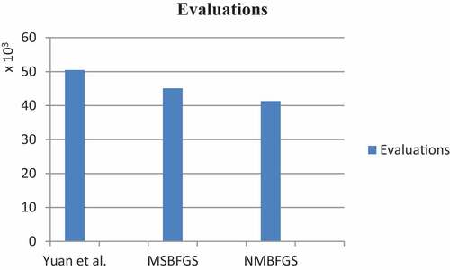
Figure 2. Overall iterations.

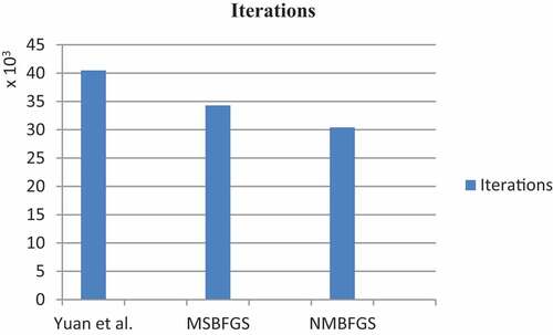
Figure 3. Overall timings.

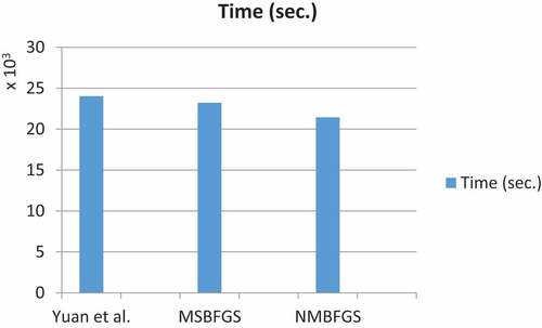
Table 3. Overall iteration, function evaluations count and timing

Method	Evaluations	Iterations	Time (sec.)	Scores	Average Optim. error
Yuan et al.	51,791	41,525	29,132.91	200	1.0*E-05
	100%	100%	100%
MSBFGS	45378	34,588	23,506.54	325	1.0*E-05
	89.35%	84.69%	96.61%
NMBFGS	41607	30,715	21,741.62	425	1.0*E-05
	81.88%	75.12%	89.21%

Table 4. Iteration, function evaluation count and timing-large problems

Method	Evaluations	Iterations	Time (sec.)	Scores	Avg. Optim. error
Yuan et al.	21,871	18,910	468.8	34	1.0*E-04
	100%	100%	100%
MSBFGS	18042	14,199	344.703	55	1.0*E-06
	82.41%	74.96%	66.53%
NMBFGS	16309	13,335	327.412	84	1.0*E-05
	74.45%	70.36%	61.87%

Table 5. Iteration, function evaluation count and timing-moderately large problems

Method	Evaluations	Iterations	Time (sec.)	Scores	Avg. Optim. error
Yuan et al.	11,264	8509	3009.78	95	1.0*E-05
	100%	100%	100%
MSBFGS	9855	7105	2529.59	134	1.0*E-04
	87.38%	83.31%	83.51%
NMBFGS	9311	6989	2375	173	1.0*E-06
	82.51%	81.93%	78.20%

Table 6. Iteration, function evaluations count and timing-medium problems

Method	Evaluations	Iterations	Time (sec.)	Scores	Avg. Optim. error
Yuan et al.	10,311	9716	16,311.66	31	1.0*E-04
	100%	100%	100%
MSBFGS	9270	8977	11,499.19	99	1.0*E-05
	89.81%	92.32%	70.32%
NMBFGS	7909	6101	10,112.13	134	1.0*E-05
	76.48%	62.39%	61.68%

Table 7. Iteration, function evaluation count and timing-small problems

Method	Evaluations	Iterations	Time (sec.)	Scores	Avg. Optim. error
Yuan et al.	8345	4390	9342.67	40	1.0*E-05
	100%	100%	100%
MSBFGS	8211	4307	9133.06	37	1.0*E-05
	98.39%	98.11%	97.76%
NMBFGS	8078	4290	8927.08	34	1.0*E-05
	96.80%	97.72%	95.55%

For all the methods tested here, the next point $x_{i+1}$ is obtained from $x_i$ by employing a line search algorithm that applies safeguarded cubic interpolation with step-doubling, such that the conditions in (4) are satisfied.

For the standard BFGS method, it is well known that a necessary and sufficient condition for ensuring that the generated updated matrices $\left\{H_i\right\}$ are positive definite and hence the computed search direction is downhill, is that $s_i^T{y}_i>0$ (Broyden, 1970). By analogy, for the new method MSBFGS, condition (24) is imposed in order to guarantee that ${\bar{v}}_i^T{z}_i$ is “sufficiently” positive to circumvent any potential numerical instability in the construction of $H_{i+1}$. Should condition (24) fail to hold, the algorithm reverts to using an MSBFGS iteration on that particular instance. An initial scaling is applied to the start inverse Hessian approximation using the methods introduced in Shanno and Phua (1978).

It is generally known that $s_i^T{y}_i>0$ is a necessary and sufficient condition for assuring that the generated updated matrices $\left\{H_i\right\}$ are positive definite and thus the computed search direction is downhill for the typical BFGS method (Broyden, 1970). By analogy, condition (24) is applied for the new technique MSBFGS in order to ensure that that ${\bar{v}}_i^T{z}_i$ is “sufficiently” positive to avoid any potential numerical instability in the building of $H_{i+1}$. If condition (24) fails, the algorithm falls back to utilizing an MSBFGS iteration on that specific instance. Using the approaches proposed in Shanno and Phua (1978), an initial scaling is applied to the start inverse Hessian approximation.

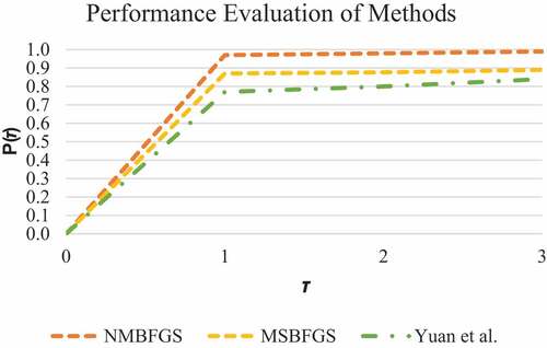
Figure 4 shows the graphical results of the test problems in terms of the most expensive component of the minimization process, the overall number of function/gradient evaluations. That is, we depict the proportion $p\left(\tau \right)$ of problems for which each technique is within a factor of $\tau$ the best number of evaluations for each approach. The algorithm that performs better in terms of evaluations that is within a factor of the best number of function evaluations is shown on the top curve. Figure 4 shows that NMBFGS outperforms the other two methods in terms of number of iterations and evaluations, thus making it the fastest and best performer.

Figure 4. Overall evaluations performance profile.

6. Conclusions

In this study, Secant-like approaches based on modifications to the classical Secant relation (1) are investigated, and a new non-Secant method is devised. To increase the quality of the computed Hessian approximations and, as a result, expedite convergence to a solution for a particular issue, the approach employs nonlinear quantities that integrate data readily available from the previous three iterations. The outperforming algorithm has been justified both theoretically and practically. The primary motivation to exploring alternatives to the standard Secant equation has been to obtain possibly better Hessian approximations that expedite the convergence of quasi-Newton methods. The proposed algorithm’s convergence behaviour has been investigated. The numerical data achieved above have shown promising results, drawing attention to the methods’ potential practical significance. The findings demonstrate that past iteration data, such as function values, gradient points, and step vectors, yield performance gains practically, and hence provide incentives to explore them further.

7. Future work

Future research ought to concentrate on modified Secant methods for various τ-parameter choices in order to investigate the numerical behaviour of these methods’ sensitivity to such choices. It would also be interesting to study these methods’ ability to offer equivalent improvements when used to solve systems of non-linear equations, as well as their convergence characteristics.

Similar approaches are also being investigated, in which the computed search direction $d_i$ is adjusted before the line search is performed. This strategy looks to be effective. A variation of the technique is also being considered, in which the update of the Hessian approximation is skipped every other iteration (or more frequently). Also, the sensitivity of the algorithmic behaviour to the accuracy of the line search deserves investigation. The numerical performance of such methods when replacing the line search with Trust Region methods is also worth exploring.

Disclosure statement

No potential conflict of interest was reported by the author(s).

Additional information

Funding

The author received no direct funding for this research.

Notes on contributors

Issam A.R. Moghrabi

Dr. Issam Moghrabi is a Professor of M.I.S/C.S. He laid the foundations of the M.B.A Program at GUST. He is a Fulbright Scholar and did a postdoctoral research in Geographic Information Systems. His main research interests are in mathematical Optimization, Management Science and Information Retrieval and database systems. He serves as a referee for many well-known journals in his subjects of interest.

References

- Al-Baali, M. (1985). New property and global convergence of the Fletcher–Reeves method with inexact line searches. IMA Journal of Numerical Analysis, 5(1), 122–19. https://doi.org/10.1093/imanum/5.1.121
- Awasthi, A., & Omrani, H. (2019). A goal-oriented approach based on fuzzy axiomatic design for sustainable mobility project selection. International Journal of Systems Science: Operations & Logistics, 6(1), 86–98. https://doi.org/10.1080/23302674.2018.1435834
- Broyden, C. G. (1970). The convergence of a class of double-rank minimization algorithms - Part 2: The new algorithm. IMA Journal of Applied Mathematics, 6(3), 222–231. https://doi.org/10.1093/imamat/6.3.222
- Dai, Y., Yuan, J., & Yuan, Y. (2002). Modified two-point step size Gradient methods for unconstrained optimization. Computational Optimization and Applications, 22(1), 103–109. https://doi.org/10.1023/A:1014838419611
- Dennis, J. E., & Schnabel, R. B. (1979). Least change Secant updates for quasi-Newton methods. SIAM Review, 21(4), 443–459. https://doi.org/10.1137/1021091
- Fletcher, R. (1970). A new approach to variable metric algorithms. The Computer Journal, 13(3), 317–322. https://doi.org/10.1093/comjnl/13.3.317
- Fletcher, R. (1987). Practical Methods of Optimization (second ed.). Wiley.
- Fletcher, R. (1994). An Overview of Unconstrained Optimization. In E. Spedicato (Ed.), Algorithms for Continuous Optimization. NATO ASI Series (Series C: Mathematical and Physical Sciences) (Vol. 434, pp. 109–143). Springer.
- Ford, J. A., & Moghrabi, I. A. R. (1993). Alternative parameter choices for multi-step quasi-Newton methods. Optimization Methods & Software, 2(3–4), 357–370. https://doi.org/10.1080/10556789308805550
- Ford, J. A., & Moghrabi, I. A. R. (1994). Multi-step quasi-Newton methods for optimization. Journal of Computational and Applied Mathematics, 50(1–3), 305–323. https://doi.org/10.1016/0377-0427(94)90309-3
- Ford, J. A., & Moghrabi, I. A. R. (1996). Using function-values in multi-step quasi-Newton methods. Journal of Computational and Applied Mathematics, 66(1–2), 201–211. https://doi.org/10.1016/0377-0427(95)00178-6
- Gharaei, A., Hoseini, S. S., & Karimi, M. (2020). Modelling And optimal lot-sizing of the replenishments in constrained, multi-product and bi-objective EPQ models with defective products: Generalised Cross Decomposition. International Journal of Systems Science: Operations & Logistics, 7(3), 262–274. https://doi.org/10.1080/23302674.2019.1574364
- Gharaei, A., Naderi, B., & Mohammadi, M. (2015). Optimization of rewards in single machine scheduling in the rewards-driven systems.Management. Science Letters, 5(6), 629–638.
- Gharaei, A., Naderi, B., & Mohammadi, M. (2019). An integrated multi-product, multi-buyer supply chain under penalty, green, and quality control polices and a vendor managed inventory with consignment stock agreement: The outer approximation with equality relaxation and augmented penalty algorithm. Applied Mathematical Modelling, 69 2 , 223–254. https://doi.org/10.1016/j.apm.2018.11.035
- Gharaei, A., Shekarabi, S. A., Karimi, M., Pourjavad, E., & Amjadian, A. (2021). An integrated stochastic EPQ model under quality and green policies: Generalised cross decomposition under the separability approach. International Journal of Systems Science: Operations & Logistics, 8(2), 119–131. https://doi.org/10.1080/23302674.2019.1656296
- Hassan, B., & Ghada, M. (2020). A new quasi-newton equation on the gradient methods for optimization minimization problem. Indonesian Journal of Electrical Engineering and Computer Science, 19(2), 737–744. https://doi.org/10.11591/ijeecs.v19.i2.pp737-744
- Hassan, B., & Mohammed, W. T. (2020). A new variants of quasi-newton equation based on the quadratic function for unconstrained optimization. Indonesian Journal of Electrical Engineering and Computer Science, 19(2), 701–708. https://doi.org/10.11591/ijeecs.v19.i2.pp701-708
- Hassan, B. (2019). A new Quasi-Newton Updating formula based on the new quasi-Newton equation. Numerical Algebra Control and Optimization, 4(1), 63–72.
- Hassan, B. (2020). A new type of quasi-Newton updating formulas based on the new quasi-Newton equation. SIAM Journal Numerical Algebra, Control, and Optimization, 10(2), 227–235. https://doi.org/10.3934/naco.2019049
- Jin, Q., & Mokhtari, A. (2021). Non-asymptotic super linear convergence of standard quasi-Newton methods. Journal of Strategic Decision Sciences, 121, https://arxiv.org/pdf/2003.13607v1.pdf
- Li, D., & Fukushima, M. (2001). A modified BFGS method and its global convergence in nonconvex minimization. Journal of Computational and Applied Mathematics, 129(1–2), 15–35. https://doi.org/10.1016/S0377-0427(00)00540-9
- Moghrabi, I. A. R. (2017). Implicit extra-update multi-step quasi-newton methods. International Journal of Operational Research, 28(2), 69–81. https://doi.org/10.1504/IJOR.2017.081472
- Moré, J. J., Garbow, B. S., & Hillstrom, K. E. (1981). Testing unconstrained optimization software. ACM Transactions on Mathematical Software, 7(1), 17–41. https://doi.org/10.1145/355934.355936
- Ortiz, F., Simpson, J. R., Pignatiello, J. J., & Heredia-Langner, A. (2004).A genetic algorithm approach to multiple-response optimization. Journal of Quality Technology, 36(4), 432–450. https://doi.org/10.1080/00224065.2004.11980289
- Sayyadi, R., & Awasthi, A. (2018). A simulation-based optimisation approach for identifying key determinants for sustainable transportation planning. International Journal of Systems Science: Operations & Logistics, 5(2), 161–174. https://doi.org/10.1080/23302674.2016.1244301
- Shanno, D. F., & Phua, K. H. (1978). Matrix conditioning and nonlinear optimization. Mathematical Programming, 14(1), 149–160. https://doi.org/10.1007/BF01588962
- Shanno, D. F. (1978). On the convergence of a new conjugate gradient algorithm. SIAM Journal on Numerical Analysis, 15(6), 1247–1257. https://doi.org/10.1137/0715085
- Tajadod, M., Abedini, M., Rategari, A., & Mobin, M. (2016). A comparison of multi-criteria decision making approaches for maintenance strategy selection (a case study). International Journal of Strategic Decision Sciences, 7(3), 51–56. https://doi.org/10.4018/IJSDS.2016070103
- Wei, Z., Li, G., & Qi, L. (2004). The superlinear convergence of a modified BFGS- type method for unconstrained optimization. Computational Optimization and Applications, 29(3), 315–332. https://doi.org/10.1023/B:COAP.0000044184.25410.39
- Wei, Z., Li, G., & Qi, L. (2006). New quasi-Newton methods for unconstrained optimization problems. Mathematics Program Applied Mathematics and Computation, 175(2), 1156–1188. https://doi.org/10.1016/j.amc.2005.08.027
- Xiao, Y. H., Wei, Z. X., & Zhang, L. (2006). A modified BFGS method without line searches for nonconvex unconstrained optimization. Advances in Theoretical and Applied Mathematics, 1(2), 149–162. https://www.ripublication.com/Volume/atamv1n2.htm
- Yuan, G., Sheng, Z., Wang, B., Hu, W., & Li, C. (2018). The global convergence of a modified BFGS method for nonconvex functions. Journal of Computational and Applied Mathematics, 327(1), 274–294. https://doi.org/10.1016/j.cam.2017.05.030
- Yuan, G., Wei, Z., & Lu, X. (2017). Global convergence of BFGS and PRP methods under a modified weak Wolfe–Powell line search. Applied Mathematical Modelling, 47(2), 811–825. https://doi.org/10.1016/j.apm.2017.02.008
- Yuan, G., Wei, Z., & Wu, Y. (2010). Modified limited memory BFGS method with non-monotone line search for unconstrained optimization. Journal of the Korean Mathematical Society, 47(4), 767–788. https://doi.org/10.4134/JKMS.2010.47.4.767
- Yuan, G., & Wei, Z. (2010). Convex minimizations. Computational Optimization and Applications, 47(1), 237–255. https://doi.org/10.1007/s10589-008-9219-0
- Zhang, J. Z., Deng, N. Y., & Chen, L. H. (1999). Quasi-Newton equation and related methods for unconstrained optimization. Journal of Optimization Theory and Applications, 102(1), 147–167. https://doi.org/10.1023/A:1021898630001