Evaluation drag coefficients for circular patch vegetation with different riverbed roughness

Abstract

The drag coefficient of a one-line circular patch of emergent sparse vegetation in an open-channel flow or riverbeds with varying bed roughness sizes was experimentally investigated. The total roughness of the channel was accounted for using the rate of energy dissipation that incorporated resistance by bed particles and cylinder obstacles. A total of 48 flume experiments were conducted by varying the flow rate, bed roughness, and water depth. The analysis of flow resistance due to the one-line patch of sparse vegetation and the variation in bed roughness was achieved through dimensional analysis. The results show that the drag coefficient C_d is a function of stem Reynolds number, Rd, Froude number, Fr, and the ratio between stem diameter and flow depth (d/H). Experiments showed that the drag coefficient varied with the stem Reynolds number, Froude number, and bed roughness. The C_d generally increased with decreasing stem Reynolds number and Froude number, and this increase in drag coefficient appeared significant for a rough bed of large particles. Results showed that Reynold numbers for different bed roughness had a minimal influence on the drag coefficients. The Fr increases as bed materials are smoother. Statistical regression analysis was achieved to drive the relationship between drag coefficient versus Rd, Fr, and d/H with a coefficient of determination of more than 0.97.

Keywords:

• Vegetation
• BED roughness
• drag coefficient
• stem Reynolds number

PUBLIC INTEREST STATEMENT

“The exclusive goal of this research was to investigate the influence of circular patch vegetation on drag coefficient for different riverbeds or irrigation canal beds roughness. A total of 48 flume experiments were conducted to mimic the field condition by varying the flow rate, bed roughness, and water depth. Dimensional analysis was performed to achieve the analysis of flow resistance due to the one-line patch vegetation and the variety in bed roughness. Experiments showed that the drag coefficient varied with the stem Reynolds number, Froude number, and bed roughness. We believe that the results of this research showed the non-dimensional terms have a clear effect on the channels smooth bed, and the effect of the Froude number is small compared to the stem Reynolds number for the vegetative patch at the bottom of the channels of mixed coarse and fine gravel and fine gravel materials.”

1. Introduction

Vegetation in natural rivers, floodplains, and irrigation canals exerts a crucial effect on the ecological environment in many respects. The growth of aquatic plants in rivers and natural streams causes an increase in water level and in the flow velocity around a vegetation patch, attenuates flood discharge, and controls the quantity of sediments due to blockage (Al-Husseini et al., 2020; Liu & Zeng, 2016; Mulahasan et al., 2021). Vegetation in aquatic ecosystems can be found in different configurations and alignments (Cheng & Nguyen, 2011; Cornacchia et al., 2018; Coscarella et al., 2021; D’Ippolito et al., 2019; Gong et al., 2019; Mulahasan & Stoesser, 2016; Mulahasan et al., 2017; Tanino & Nepf, 2008; Wang et al., 2014).

A circular patch of vegetation may be found in natural rivers as an isolated patch (Chang & Constantinescu, 2015; Cheng et al., 2019; Takemura & Tanaka, 2007; Tanaka & Yagisawa, 2010; Tanaka et al., 2007), neighboring patches (Cornacchia et al., 2018; Kitsikouds et al., 2020; De Lima et al., 2015) or may be found as a one-line circular patch of vegetation (Li et al., 2020; Yokojima et al., 2014). Flow and turbulence structures through an isolated circular patch of vegetation was numerically investigated by a number of researchers (Chang & Constantinescu, 2015, 2015; Kim et al., 2018; Yu et al., 2013, 2014, 2013; Zhang et al., 2019), and experimentally examined by (Cheng et al., 2019; Kitsikouds et al., 2020; Zong & Nepf, 2011, 2012). Flow and turbulence in the wake of neighboring rigid and emergent circular patches of vegetation were experimentally examined by Kitsikouds et al. (2020) and numerically by Lima et al. (De Lima et al., 2015) using Computational Fluid Dynamics (CFD) response. Cornacchia et al. (2018) determined that neighboring patches tend to grow in a slightly angled line, and an isolated patch was found to grow in V-like shapes to reduce drag forces. The disagreement between the numerical large eddy simulation model and the experimental data was attributed to the uniform distribution of the drag coefficient of a vegetation patch. Anjum and Tanaka (2019) experimentally investigated flow variation and backwater effects due to vegetation patches, changing the vegetation density and water depth. Zhou and Venayagamoorthy (2019) investigated wake dynamics of flow through a suspended cylindrical patch using large eddy simulation (LES) at deep flow conditions. Variable number of cylinders was used to study the effects of patch density on the wake dynamics.

The drag coefficient of an isolated vegetation patch was investigated by a number of academic research papers (Cheng et al., 2019; Taddei et al., 2016; Zhou & Venayagamoorthy, 2019). Generally, the drag coefficient of vegetation is influenced by the trunk and leaves due to viscosity and pressure (Albayrak et al., 2012). Flow resistance of two types of vegetation configuration (continuous or discontinuous patch of vegetation along the center-line of the flume) was investigated experimentally and numerically (Yokojima et al., 2014). Flow resistance from the combined effects of bed friction and vegetation elements was investigated (Dupuis et al., 2016). Impact of the porosity of an isolated circular vegetative patch on the drag coefficient was investigated (Cheng et al., 2019). Flow characteristics around a one-line patch of emerged vegetation located on one side of a channel was studied (Li et al., 2020). Flow resistance of floodplains vegetated by a mixture of flexible plants and grasses of low to high vegetation densities was studied by (Box et al., 2021). It was found that flow resistance by floodplain vegetation decreased by 35–90% when the submergence was increased from 1 to 2. Experimentally, the drag coefficient has been evaluated in consideration of changes in flow conditions. The analysis of the connection between vegetation and water flow is a complex issue due to the difference in physical mechanisms that influence the phenomenon and the biomechanical effects that describe different vegetation types (D’Ippolito et al., 2019).

Most previous studies were based on laboratory flume tests or numerical simulations of vegetated streams with smooth beds. A variety of bed roughness can be found in rivers and streams, such as large pebbles and gravel, so the effect of surface roughness was considered together with the growth of apparent plants above the water surface. Low-density vegetation was chosen, distributed in the form of a circular vegetation patch at equal distances along the length of the laboratory flume. This experimental study aims to evaluate the combined effects of vegetation obstacles and bed roughness on drag coefficients. A series of circular patches of emergent, sparse vegetation located at the center line of a laboratory flume with changing flow rate, water depth, and bed material size is studied. In addition, the present study will provide hydraulic characteristics of flow past free surface piercing cylinders such as drag coefficient is of particular relevance to offshore structures. The following section focuses on the flow resistance coefficient by an array of vegetation elements.

2. Materials and methods

2.1. Drag Coefficient relationships

Emergent vegetation in natural streams is usually described by its diameter, height, and area of plants. In laboratory experiments, emergent vegetation is usually mimicked by rigid stems and may be distributed in a lined, staggered, or random arrangement. Its density (λ) can be expressed by solid volume fraction (SVF) and can be expressed as follows:

(1) $\lambda =\frac{m\pi d^2}{4}$(1)

where, m is number of stems per unit bed area, and d is the stem diameter. In the vicinity of rigid vegetation in stream flows, the roughness coefficient is expressed as a function of drag force exerted by the flow on the vegetation elements, stem diameter, and velocity approach due to the different vegetation distributions as follows:

(2a) $F_D=0.5\rho C_d{A}_{veg}{v_a}^2$(2a)

(2b) $F_D=0.5\rho C_d{h}_{veg}d{v_a}^2$(2b)

where, $\rho$ is the fluid density, $C_d$ is the drag coefficient, $A_{veg}\left(=h_{veg}d\right)$ is the projected vegetation area, $v_a$ is the approach velocity, $h_v$ is the depth of immersed part of vegetation cylinder and $d$ is the vegetation diameter. The drag coefficient is a function of stem Reynolds number $Rd$, Froude number Fr, d/ H ratio, and vegetation density λ. The stem Reynolds number, $Rd$ for rigid emergent vegetation elements is defined as follows:

(3) $Rd=\frac{\rho Ud}{\mu }=\frac{Ud}{\nu }$(3)

where $\rho$ is the fluid density, $d$ is the characteristic length and here is stem diameter, $U$ is the fluid velocity, $\mu$ is fluid dynamic viscosity and $\nu$ is the fluid kinematic viscosity.

A number of relationships between the drag coefficient C_d and stem Reynolds number, Rd was extracted experimentally by Schlichting (1982) as follows:

(4a) $C_d=3.07R{d}^{-0.168},\left(Rd<800\right)$(4a)

(4b) $C_d=1,\left(800\le Rd<8000\right)$(4b)

(4c) $C_d=1.2,\left(8000<Rd<{10}^5\right)$(4c)

Different expressions of the drag coefficients are found in the literature review of the topic, as reported in the following paragraphs:

Based on drag force measurements, the drag coefficient is induced in the following expressions by Ishikawa et al. (2000), Kothyari et al. (2009), D’Ippolito et al. (2019), and Ishikawa et al. (2000) conducted experimental work on the drag force of rigid vegetation arranged in an open-channel flow with varying Froude number (Fr) and an empirical expression was presented as follows:

(5) $C_d=-0.32Fr+1.24$(5)

where, $Fr=\frac{v_a}{\sqrt{gH}},g\mathrm{i}\mathrm{s}\mathrm{t}\mathrm{h}\mathrm{e}\mathrm{a}\mathrm{c}\mathrm{c}\mathrm{e}\mathrm{l}\mathrm{e}\mathrm{r}\mathrm{a}\mathrm{t}\mathrm{i}\mathrm{o}\mathrm{n}\mathrm{d}\mathrm{u}\mathrm{e}\mathrm{t}\mathrm{o}\mathrm{g}\mathrm{r}\mathrm{a}\mathrm{v}\mathrm{e}\mathrm{t}\mathrm{y},\mathrm{a}\mathrm{n}\mathrm{d}H\mathrm{i}\mathrm{s}\mathrm{t}\mathrm{h}\mathrm{e}\mathrm{f}\mathrm{l}\mathrm{o}\mathrm{w}\mathrm{d}\mathrm{e}\mathrm{p}\mathrm{t}\mathrm{h}.$

Kothyari et al. (2009) formulated the following equation for the drag coefficient $C_d$ with Froude number $Fr$ and vegetation density λ and stem Reynolds number $Rd$ by measuring the fluid forces exerted on the cylinders by a load cell. This equation is applicable for both sub-critical and super critical flows.

(6) $C_d=1.8R{d}^{3/50}\left[1+0.45\mathrm{l}\mathrm{n}\left(1+100\lambda \right)\right]\left(0.8+0.2Fr-1.5F{r}^2\right)$(6)

For a linear arrangement of cylinders, (D’Ippolito et al., 2019) evaluated the drag coefficient in terms of vegetation density as follows:

(7) $C_d=0.211ln\left(100\lambda \right)+0.7841000<Rd<10000$(7)

Based on Ergun’s (1952) equation for both the laminar and turbulent components of the pressure loss across a packed bed, Tanino and Nepf (2008) proposed an expression for the drag coefficient of rigid circular cylinders as follows:

(8) $C_d=2\left[\frac{{\alpha }_o}{Rd}+{\alpha }_1\right]$(8)

where, ${\alpha }_o=5+313.17\lambda$, ${\alpha }_1=0.46+3.8\lambda$, $\lambda$ is the projected area occupied by the vegetation elements per unit bed area in an array of cylinders.

Tanaka and Yagisawa (2010) investigated the drag coefficient of clump- type emergent rigid vegetation with a changing number of cylinders inside the patch of vegetation and water depth. Cheng and Nguyen (2011) suggested an empirical relation between $C_d\mathrm{a}\mathrm{n}\mathrm{d}{R}_v$ through a series of experiments, as shown below:

(9) $C_d=\frac{50}{{R_v}^{0.43}}+0.7\left(1-e^{\frac{-R_v}{15000}}\right),\left(R_v=5.2-5.6\times {10}^5\right)$(9)

where $R_v=\frac{v_a{r}_v}{\upsilon },r_v$ is the vegetation-related hydraulic radius defined as $r_v=\pi d\left(\frac{1-\lambda }{4\lambda }\right)$, and $v_a$ is the velocity approaching the vegetation.

Wang et al. (2014) performed many experiments to obtain a best-fit function explaining the relationship between $C_d$ and $R_{ev}$ in a subcritical flow, as shown as follows:

(10) $C_d=\frac{90}{R{e_v}^{0.5}}+4.5\frac{d}{H}-0.303ln\lambda -0.9$(10)

where $R{e}_v$ is defined as $R{e}_v=\frac{\left(1-\lambda \right)v_{a}H}{\upsilon },$ and $\lambda =\frac{\pi N{\left(\frac{d}{2}\right)}^2}{BL}$, where N is number of stems in an array of vegetation elements.

2.2. Experimental setup

The experiments were conducted in a hydraulic recirculating plastic walled flume of 4.58 m long and 0.3 m wide and depth. The flume was set to a bed slope of 0.0005. A sharp-crested weir was installed at the end of the flume’s working section to control the flow depth. Four different flow rates of 3.21, 4.47, 5.88, and 6.90 l/s were used. Discharge values (Q) were measured and determined using a gauge reading installed on the canal pipe entering the laboratory canal. These values were checked after knowing and measuring the volume of water leaving the canal at downstream using a vessel of a known volume and a stopwatch for each laboratory experiment. This check is repeated three times for each discharge run.

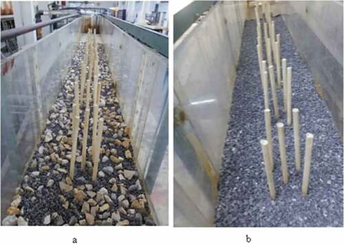
The vegetation was mimicked using sets of rigid wooden circular cylindrical rods of 1 cm in diameter. A series of vegetation patches was installed along the centre line of the flume’s working section with a 20 cm center to center distance (figure 1). The vegetation patches were designed with a diameter D = 10 cm having five cylinders (d = 1 cm) arranged as shown in figure 2. Eleven patches of cylinders were installed at 0.2 m intervals along the flume’s center line, beginning 1.2 m from the flume’s inlet (figure 2a). A control volume was chosen to include one patch and half the area before and after the patch. So, the vegetation density would be the same for the entire channel section and each control volume (figure 2b). The drag coefficient was considered due to vegetation cylinders and bed roughness. Two types of bed roughness in comparison with a smooth bed were considered; coarse gravel (4.75–9.5 mm) mixed with fine gravel (2.36–4.75 mm) and fine gravel (2.36–4.75 mm) as shown in figure 3. The size of the gravel was estimated in the laboratory using the sieve analysis method. Water depths were measured under uniform flow conditions along the mid distance among patches.

Figure 1. A photograph illustrating the experimental setup with one line circular patch of diameter, D, of vegetation with smooth bed.

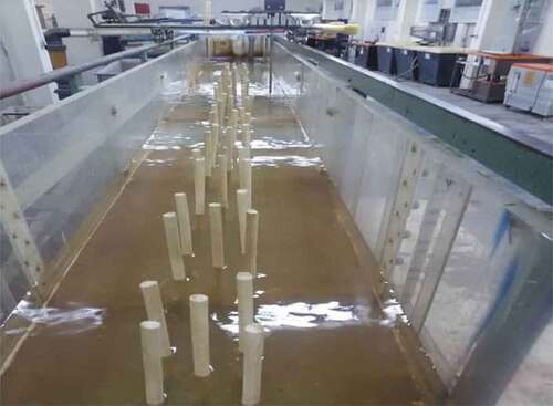
Figure 2. A) Schematic diagram of the experimental set-up, and b) Control volume of vegetation patch.

Figure 3. Bed roughness for: a) mixed sizes, and b) mono-size bed material.

2.3. Flow resistance in vegetated streams

For steady uniform flow conditions where the water-level slope is parallel to the bed slope, the driving force of the flow equates with the bed resistance and form drag according to Mulahasan and Stoesser (2016) is expressed as:

(11) $F_G=F_f+F_D$(11)

where $F_G=\rho gSH\left(1-m\frac{\pi d^2}{4}\right)$ is the gravitational force $F_f={\tau }_b\left(1-m\frac{\pi d^2}{4}\right)$, is the wall friction drag force, and $F_D=\frac{1}{2}m\rho C_{d}Hd{U}^2$ is the drag force exerted by the vegetation. From the definition of each term in Equation (11)(11) $F_G=F_f+F_D$(11) , the following results are obtained:

(12) $\rho gSH\left(1-m\frac{\pi d^2}{4}\right)={\tau }_b\left(1-m\frac{\pi d^2}{4}\right)+\frac{1}{2}m\rho C_{d}Hd{U}^2$(12)

where $\rho$ is the fluid density, $g$ is the gravitational acceleration, S is the bed slope, H is the flow dept ${\tau }_b=\rho gRS\mathrm{i}\mathrm{s}\mathrm{b}\mathrm{e}\mathrm{d}\mathrm{s}\mathrm{h}\mathrm{e}\mathrm{a}\mathrm{r}\mathrm{s}\mathrm{t}\mathrm{r}\mathrm{e}\mathrm{s}\mathrm{s},$ h, d is the stem diameter, R is the hydraulic radius = A/P, A is cross section area of non-vegetated channel, P is wetted parameter for non-vegetated channel, L is the reach length, and U is the bulk velocity defined as

(13) $U=\frac{QL}{\left(A_b-A_g\right)H}$(13)

where $,A_b=WL$ is the total frictional bed area $,W$ is the channel width, and $A_g=N\frac{\pi d^2}{4}$ is the bed area occupied by stems. Equations 12(12) $\rho gSH\left(1-m\frac{\pi d^2}{4}\right)={\tau }_b\left(1-m\frac{\pi d^2}{4}\right)+\frac{1}{2}m\rho C_{d}Hd{U}^2$(12) and 13(13) $U=\frac{QL}{\left(A_b-A_g\right)H}$(13) were used in calculating the drag coefficient after measuring and calculating the other variables from the practical results in the laboratory. It is noted that the values of S = 1/2000, N = 5. The properties of liquid used (water) are: $\rho =1000\frac{kg}{m^3},\mu =1.002\times {10}^{-3}\frac{N}{m^2}.s,\upsilon =1.002\times {10}^{-6}\frac{m^2}{s}$, and the rest of the variables were measured in the laboratory. The only value of the drag coefficient was calculated for each laboratory experiment.

2.4. Dimensional analysis

The relationships between vegetation and resistance under different conditions, such as bed roughness, plant diameter, flow velocity, water depth, and fluid properties, were examined. We assumed that the drag coefficient depends on the variables of water density, water viscosity, gravitational acceleration, depth of water H, flow velocity u, and stem diameter d, and it is expressed as follows:

(14) $C_d=f\left(\rho ,\mu ,g,H,u,d\right)$(14)

The dimensionless numbers of parameters were determined through Buckingham’s $\pi$-theorem dimensional analysis; C_d simulated using dimensionless parameters, was expressed as follows (see Appendix A):

(15) $C_d=F\left(Rd,Fr,\frac{d}{H}\right)$(15)

Forty-eight series of experimental data were performed in a subcritical flow and used them to calculate Cd for patches of vegetation located along the centre line working section of the laboratory flume. Equations were formulated for different bed roughness using the Statistical Package for Social Science (SPSS) software programme (version 24). Equation 15(15) $C_d=F\left(Rd,Fr,\frac{d}{H}\right)$(15) from the dimensional analysis was used to derive an equation for the drag coefficient through the experiments conducted.

3. Results

The results of laboratory experiments for various different flows (Q = 3.21, 4.47, 5.88, and 6.90 l/s) were as follows..

3.1. Water surface waves

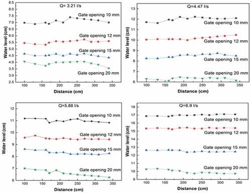
In consideration of free-surface waves, the changes in water levels in the part of the populated flume should be monitored using rods and the fluctuation in surface water around each single rod should be regulated. Flow depth was calculated as an average value through the flume reach using a point gauge with an accuracy of 0.10 mm. Figure 4 shows the measured water-level profile along the entire channel for four discharges at different gate openings of 10 mm, 12 mm, 15 mm, and 20 mm for each discharge of flow. From Figure 4, the water level in the channel increases with the increase in the water discharge at the given gate opening. That is evident for all other gate openings. For example, if the amount of flow discharge is 3.2 l/s and the gate opening is 10 mm, the water level in the channel is about 7 cm. When flow discharge is 4.4 l/s, the water level is about 12 cm. Increasing the flow discharge to 9.6 l/s produces the water level is about 17 cm for the same gate opening of 10 mm. Increasing flow discharge in the presence of vegetation leads to an increase in water level in the canal.

Figure 4. Variations of water levels along the canal for different discharges.

3.2. Bed roughness

To demonstrate the effect of the bed roughness of the channel on the calculation of the drag coefficient, three types of beds were used in the channel, as follows:

- Smooth bed

- Mixed coarse (size 4.75–9.5 mm) and fine gravels (size 2.36–4.75 mm) bed, and

- Fine gravels (size 2.36–4.75 mm) bed.

3.3. Drag coefficient,${\mathit{C}}_{\mathit{d}}$

The results of the drag coefficient were obtained for the bed of the canal and for the various depths of water and discharges under the conditions of the different gate openings as shown in the Table (1–3) in an Appendix using equation 10(10) $C_d=\frac{90}{R{e_v}^{0.5}}+4.5\frac{d}{H}-0.303ln\lambda -0.9$(10) . Many laboratory experiments were conducted with consideration given to the effect of the drag coefficient in various conditions such as plant presence, flow velocity and flow depth in the canal. From the previously performed dimensional analysis (Equation 13(13) $U=\frac{QL}{\left(A_b-A_g\right)H}$(13) ), the first dimensional variable affecting the drag coefficient values is the stem Reynolds number, $Rd$. This non-dimensional variable was calculated through field experiments for different bed roughness in preparation for finding a relationship between this dimensionless variable and the drag coefficient, and this relation represented in figure 5 was drawn. Reynolds number, $R_H$ depends on the depth of flow instead of the diameter of the cylinder used as a plant and its effect on the calculation of the drag coefficient. figure 6 shows the variation of the Reynolds number, $R_H$ and the drag coefficient are given for the various roughness of the channel bed surface. Froude number is the second dimensional variable affecting the drag coefficient, according to the equation of equation 13(13) $U=\frac{QL}{\left(A_b-A_g\right)H}$(13) . The $C_d$ was calculated as shown in Table 1–3, and the relationship between this number and the drag coefficient, represented in figure 7. The dimensional expression $\frac{d}{H}$ represents the last variable in the dimensional analysis affecting the values of the drag coefficient. figure 8 represents the relationship between this dimensionless expression and the drag coefficient for different bed roughness. To obtain a single relationship between drag coefficient, $C_d$ and $R_d,F_r,\frac{d}{H}$ for each type of channel bottom surface roughness, a statistical regression analysis method was used. Statistical regression analysis of the results in the form of equation (13)(13) $U=\frac{QL}{\left(A_b-A_g\right)H}$(13) was performed using the SPSS software programme (version 24). The drag coefficient was calculated as in the following equations. For a smooth bed, the drag coefficient was defined as follows with R² of 0.977:

(16) $C_d=11.457R{d}_{\hspace{0.17em}}^{0.072}+0.482F{r}_{\hspace{0.17em}}^{-1.196}+0.887\frac{d}{H}-21.229$(16)

Table 1. Results of computing drag coefficient and experimental measurements for smooth bed

Run	Gate opening, mm	H, m	R, m	Q, l/s	U, m/s	Cd	Fr	Rd	RH
1	10	0.077	0.0298	3.21	0.289	1.438	0.332	2887	22,234
2	12	0.055	0.0288	3.21	0.303	1.026	0.410	3025	16,731
3	15	0.045	0.0282	3.21	0.310	0.760	0.467	3104	13,968
4	20	0.039	0.0279	3.21	0.314	0.568	0.507	3140	12,278
5	10	0.12	0.213	4.47	0.213	2.599	0.196	2127	25,529
6	12	0.102	0.250	4.47	0.250	1.814	0.250	2504	25,539
7	15	0.085	0.309	4.47	0.309	1.165	0.339	3092	26,285
8	20	0.063	0.366	4.47	0.366	0.718	0.465	3658	23,119
9	10	0.112	0.062	5.88	0.187	2.502	0.178	1868	20,887
10	12	0.095	0.059	5.88	0.202	1.812	0.209	2019	19,183
11	15	0.083	0.052	5.88	0.250	1.189	0.277	2501	20,829
12	20	0.061	0.044	5.88	0.313	0.545	0.404	3127	19,073
13	10	0.17	0.078	6.9	0.143	5.203	0.111	1428	24,280
14	12	0.154	0.074	6.9	0.157	4.121	0.128	1567	24,139
15	15	0.125	0.068	6.9	0.188	2.540	0.170	1882	23,528
16	20	0.1	0.058	6.9	0.245	1.366	0.248	2450	24,425

Table 2. Results of computing drag coefficient and experimental measurements for bed of mixed coarse and fine gravels

Run	Gate opening, mm	H, m	R, m	Q, l/s	U, m/s	Cd	Fr	Rd	RH
17	10	0.072	0.048	3.21	0.146	3.056	0.174	1459	10,482
18	12	0.064	0.042	3.21	0.176	2.140	0.223	1761	11,204
19	15	0.058	0.041	3.21	0.181	1.756	0.239	1811	10,578
20	20	0.058	0.041	3.21	0.184	1.732	0.244	1839	10,702
21	10	0.128	0.069	4.47	0.122	6.102	0.109	1217	15,559
22	12	0.104	0.061	4.47	0.150	3.609	0.148	1499	15,663
23	15	0.084	0.053	4.47	0.191	2.025	0.210	1907	16,106
24	20	0.070	0.047	4.47	0.227	1.253	0.274	2270	15,887
25	10	0.144	0.074	5.88	0.112	7.491	0.095	1125	16,166
26	12	0.115	0.065	5.88	0.143	4.176	0.134	1425	16,423
27	15	0.093	0.055	5.88	0.187	2.265	0.196	1873	17,481
28	20	0.077	0.049	5.88	0.229	1.386	0.263	2289	17,712
29	10	0.176	0.081	6.9	0.108	9.145	0.082	1076	18,950
30	12	0.141	0.071	6.9	0.139	5.006	0.118	1391	19,621
31	15	0.116	0.064	6.9	0.171	3.005	0.161	1713	19,803
32	20	0.086	0.053	6.9	0.231	1.409	0.251	2306	19,795

Table 3. Results of computing drag coefficient and experimental measurements for bed of mono-size fine gravels

Run	Gate opening, mm	H, m	R, m	Q, l/s	U, m/s	Cd	Fr	Rd	RH
33	10	0.069	0.047	3.21	0.152	2.693	0.185	1525	10,554
34	12	0.061	0.042	3.21	0.180	1.904	0.232	1798	10,992
35	15	0.059	0.041	3.21	0.188	1.723	0.247	1879	11,070
36	20	0.058	0.040	3.21	0.189	1.672	0.251	1894	11,023
37	10	0.131	0.070	4.47	0.117	6.686	0.103	1166	15,248
38	12	0.108	0.061	4.47	0.151	3.755	0.147	1509	16,221
39	15	0.087	0.052	4.47	0.195	2.087	0.211	1946	16,851
40	20	0.071	0.046	4.47	0.234	1.292	0.279	2337	16,667
41	10	0.155	0.076	5.88	0.109	8.373	0.089	1092	16,949
42	12	0.127	0.068	5.88	0.136	4.928	0.122	1358	17,210
43	15	0.100	0.060	5.88	0.168	2.766	0.170	1684	16,874
44	20	0.080	0.051	5.88	0.217	1.480	0.246	2173	17,279
45	10	0.185	0.085	6.9	0.096	11.620	0.071	957	17,740
46	12	0.151	0.075	6.9	0.123	6.529	0.101	1228	18,596
47	15	0.126	0.068	6.9	0.150	4.024	0.135	1498	18,856
48	20	0.091	0.056	6.9	0.205	1.763	0.217	2052	18,631

Figure 5. Variation of C_d with stem Reynolds number, R_d.

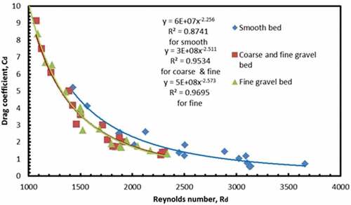
Figure 6. Variation of Cd with Reynolds number, $R_H$ with vegetation.

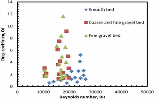
Figure 7. Variation of drag coefficient, C_d with Froude number, F_r.

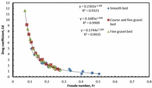
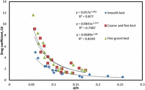
Figure 8. Variation of drag coefficient, C_d with d/H ratio.

For mixed coarse and fine gravels, the drag coefficient was expressed as follows R² of 0.994:

(17) $C_d=4.938\times {10}^{10}R{d}^{-3.244}+48.214F{r}_{\hspace{0.17em}}^{521.473}-11.946\frac{d}{H}+2.362$(17)

For mono-sized fine gravel materials, the drag coefficient was as follows R² of 0.997:

(18) $C_d=4.3266\times {10}^{9}R{d}^{-2.894}+42.407F{r}_{\hspace{0.17em}}^{515.494}-11.289\frac{d}{H}+2.036$(18)

4. Discussion

The measurements were used in the water balance equation to evaluate the drag coefficient; C_d. Figure 4 shows the measured water-level profile along the entire channel for four discharges at different gate openings in the vicinity of a series of vegetated patches. The figure demonstrates that vegetation has a significant impact on water depth; that is, for a given discharge, the water depth increases in front of the vegetation elements. The presence of vegetation in the channel exerts an effect on the relationship of variations in water level with distance curve compared with the case without vegetation. Consequently, increases in water depths affect the drag coefficient. Forty-eighty runs of experiments were completed. The measurements of total drag coefficients for all cases are summarised in Table 1–3 with smooth bed, coarse and fine gravel bed; and fine gravel bed, respectively. The values of the drag coefficient ${\mathit{C}}_{\mathit{d}}$ were calculated in Table (1–3), depending on equation 10(10) $C_d=\frac{90}{R{e_v}^{0.5}}+4.5\frac{d}{H}-0.303ln\lambda -0.9$(10) . These tables illustrate the use of four different water discharges, and for each amount, four openings for the gate were used at the downstream of the canal (10, 12, 15, and 20 cm) to demonstrate the effect of the different hydraulic conditions in the presence of the plant on the calculation of the drag coefficient.

figure 5 depicts the behaviour of C_d with stem Reynolds number, Rd for different bed roughness of a one-line patch of vegetation. The figure indicates that the highest drag coefficient, C_d of coarse and fine gravel bed materials shows a minimum stem Reynolds number, Rd and that C_d decreases with increasing Rd for all experiments runs. Figure 5 also shows a match between two curves of mixed fine gravels with coarse gravels and mono-sized fine gravels. This is one of the results we have obtained, as shown in equations 17(17) $C_d=4.938\times {10}^{10}R{d}^{-3.244}+48.214F{r}_{\hspace{0.17em}}^{521.473}-11.946\frac{d}{H}+2.362$(17) and 18(18) $C_d=4.3266\times {10}^{9}R{d}^{-2.894}+42.407F{r}_{\hspace{0.17em}}^{515.494}-11.289\frac{d}{H}+2.036$(18) , the two cases are similar for the presence of gravel with sand in both cases, with the different nature of the roughness of the materials. At high values of Rd, the drag coefficient, C_d tends to become constant, and this result is similar to those of D’Ippolito et al. (2019; Kothyari et al. (2009). figure 6 presents the variation in drag coefficient, C_d with Reynolds number based on water depth; R_H ranges between 10,500 and 26,300. The figure shows that the drag coefficient C_d increases with roughness, remaining constant with R_H. The same results were also obtained by D’lppolito et al. (2019). figure 7 shows the variation in drag coefficient with the Froude number Fr, which indicates that C_d decreases with increasing Fr, similar to the variation in Reynolds number, R_d versus drag coefficient. The second term in the water balance equation (equation 11(11) $F_G=F_f+F_D$(11) ) is the bed shear stress that plays a significant role in flow resistance. It can be said that the coarse and fine gravel bed surface and fine gravel bed surface are more valuable for the drag coefficient due to the presence of roughness compared with the smooth surface bed as shown in Figures 5 and 7.

The dimensional analysis indicates in Equation (15)(15) $C_d=F\left(Rd,Fr,\frac{d}{H}\right)$(15) that the drag coefficient, C_d is a function of the ratio d/H. figure 8 depicts the relationship between the dimensionless d/H and drag coefficient, C_d. The trend shows that C_d decreases with increasing d/H, as approximated by Morinaqa et al. (2012) for one-line trees. This relationship is illustrated in figure 8 and Equation 16(16) $C_d=11.457R{d}_{\hspace{0.17em}}^{0.072}+0.482F{r}_{\hspace{0.17em}}^{-1.196}+0.887\frac{d}{H}-21.229$(16) . The drag coefficient decreases with an increase in the ratio d/H. As the depth of the water decreases with the stability of the cylinder diameter, this ratio increases, resulting in a lower drag coefficient. figure 8 shows that the higher roughness gives a greater drag coefficient than the smooth surface bed for the same ratio d/H. In general, vegetation drag coefficients with a rough bed illustrate higher values than those with a smooth bed. Statistical regression analysis was used to examine the effect of various hydraulic conditions such as flow velocity, flow depth, as well as the presence of plants within the channel during the flow of water. Mathematical relationships were derived to represent the roughness of the channel bed surface and its effect under these different hydraulic conditions. The equations (16(16) $C_d=11.457R{d}_{\hspace{0.17em}}^{0.072}+0.482F{r}_{\hspace{0.17em}}^{-1.196}+0.887\frac{d}{H}-21.229$(16) –18(18) $C_d=4.3266\times {10}^{9}R{d}^{-2.894}+42.407F{r}_{\hspace{0.17em}}^{515.494}-11.289\frac{d}{H}+2.036$(18) ) show that the coefficient of determination (${\mathrm{R}}^2$) is higher than 90%, which indicates the strength of the correlation of the drag coefficient with the measured dimensionless variables ($Rd,Fr,\frac{d}{H})$. It was noticed from Equations 15(15) $C_d=F\left(Rd,Fr,\frac{d}{H}\right)$(15) and 16(16) $C_d=11.457R{d}_{\hspace{0.17em}}^{0.072}+0.482F{r}_{\hspace{0.17em}}^{-1.196}+0.887\frac{d}{H}-21.229$(16) that the variable R_d has a greater effect than the other non-dimensional variables. This indicates that the presence of vegetation is more influential in calculating the drag coefficient than the Fr number and the ratio d/H. The Froude number (Fr) has the least effect on the drag coefficient in the mixed coarse and fine gravels bed and mono-sized fine gravel material bed, while its effect is visible on the smooth ground bed. Equation (16)(16) $C_d=11.457R{d}_{\hspace{0.17em}}^{0.072}+0.482F{r}_{\hspace{0.17em}}^{-1.196}+0.887\frac{d}{H}-21.229$(16) shows that there is a clear influence of the three dimensionless variables ($Rd,Fr,\frac{d}{H})$ for a smooth bed.

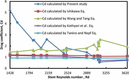
figure 9 shows the comparison in the values of the drag coefficient of the various equations for the previous studies with the equation derived in the current study of the state of the smooth bed roughness by statistical regression analysis. It is evident from the figure that there is a good convergence in the values of the drag coefficient of the current study with the previous studies at high Reynolds numbers. It can also be noted that the Kothyari et al. (2009) equation is the closest to the values of the drag coefficient for the current study. Figure 9 indicates that in the lower Reynolds values, the values of the drag coefficient are high compared to previous studies due to the differences in vegetation density for each study.

Figure 9. Comparison of calculated drag coefficient with previous studies.

5. Conclusions

The drag coefficient in the vicinity of rigid emergent vegetation with different bed roughness was studied experimentally. Eleven patches of rigid circular cylinders and three types of bed roughness (smooth, coarse and fine, and fine) were used. The main result of this study showed that within the experimental range conducted, the drag coefficient for the coarse and fine beds was greater than that for other bed roughnesses at a minimum stem Reynolds number, R_d. All experimental runs indicated that the drag coefficient, C_d decreased with increasing stem Reynolds number, R_d, and remained constant at high R_d for all bed roughness. The drag coefficients were investigated independently of the Reynolds number; when Reynolds number varied from 10,500 to 26,300. The results show that the drag coefficient C_d of the coarse and fine gravel bed and other surface fine gravel bed is more valuable than that of the smooth bed. The statistical program (SPSS) was used, and nonlinear equations were found through the method of regression analysis, and the correlation coefficient in these equations was above 90%, which indicates the strength of the correlation to find the drag coefficient with the non-dimensional variables. These non-dimensional terms have a clear effect on the channel’s smooth bed, and the effect of the Froude number is small compared to the stem Reynolds number for the vegetative patch at the bottom of the channels of mixed coarse and fine gravel and fine gravel materials. When comparing the statistical regression analysis (equations 16(16) $C_d=11.457R{d}_{\hspace{0.17em}}^{0.072}+0.482F{r}_{\hspace{0.17em}}^{-1.196}+0.887\frac{d}{H}-21.229$(16) –18(18) $C_d=4.3266\times {10}^{9}R{d}^{-2.894}+42.407F{r}_{\hspace{0.17em}}^{515.494}-11.289\frac{d}{H}+2.036$(18) ) that were derived, it becomes clear that the effect of the Froude number for the case of a smooth bed (equation 16(16) $C_d=11.457R{d}_{\hspace{0.17em}}^{0.072}+0.482F{r}_{\hspace{0.17em}}^{-1.196}+0.887\frac{d}{H}-21.229$(16) ) is greater than the Froude number for the case of the other two surfaces (equations 17(17) $C_d=4.938\times {10}^{10}R{d}^{-3.244}+48.214F{r}_{\hspace{0.17em}}^{521.473}-11.946\frac{d}{H}+2.362$(17) and 18(18) $C_d=4.3266\times {10}^{9}R{d}^{-2.894}+42.407F{r}_{\hspace{0.17em}}^{515.494}-11.289\frac{d}{H}+2.036$(18) ).

Acknowledgements

The authors are thankful to Mustansiriyah University (www.uomustansiriyah.edu.iq) and the staff of the Hydraulic Laboratory- College of Engineering for supporting this research.

Disclosure statement

No potential conflict of interest was reported by the author(s).

Additional information

Funding

The authors received no direct funding for this research.

Appendix A

Details of Dimensional Analysis

The drag coefficient is function of water density, $\rho$, water viscosity, $\mu$, gravitational acceleration, g, depth of water H, flow velocity u, and stem diameter, d, and it is expressed as follows:

(A1) ${\mathit{C}}_{\mathit{d}}=\mathit{f}\left(\mathit{\rho },\mathit{\mu },\mathit{g},\mathit{H},\mathit{u},\mathit{d}\right)$(A1)

The dimensionless numbers of parameters were determined through Buckingham’s $\pi$-theorem dimensional analysis and assumed that repeating variables are $\rho ,U,H$. Therefore, the $\pi$ -theorem is expressed as..

(A2) ${\mathit{\pi }}_{\mathbf{1}}=C{\hspace{0.17em}}_d$(A2)

(A3) ${\mathit{\pi }}_2={\mathit{\rho }}^{\mathit{a}}\cdot {\mathit{U}}^{\mathit{b}}\cdot {\mathit{H}}^{\mathit{c}}\cdot \mathit{\mu }$(A3)

(A4) ${\mathit{\pi }}_3={\mathit{\rho }}^{\mathit{a}}.{\mathit{U}}^{\mathit{b}}.\hspace{0.17em}{\mathit{H}}^{\mathit{c}}.\mathit{g}$(A4)

(A4) ${\pi }_4={\mathit{\rho }}^{\mathit{a}}.{\mathit{U}}^{\mathit{b}}.\hspace{0.17em}{\mathit{H}}^{\mathit{c}}.\mathit{d}$(A4)

This research assumed that the dimension viraibles are mass, M, length, L, and time, T:

(A5) ${\mathit{M}}^0{\mathit{L}}^0{\mathit{T}}^0={\left(\frac{\mathit{M}}{{\mathit{L}}^3}\right)}^{\mathit{a}}.{\left(\frac{\mathit{L}}{\mathit{T}}\right)}^{\mathit{b}}.{\mathit{L}}^{\mathit{c}}.\hspace{0.17em}\frac{\mathit{M}}{\mathit{L}\mathit{T}}$(A5)

(A6a) $\mathit{M}:\mathbf{0}=\mathit{a}+\mathbf{1}$(A6a)

(A6b) $\mathit{L}:\mathbf{0}=-3\mathit{a}+\mathit{b}+\mathit{c}-\mathbf{1}$(A6b)

(A6c) $\mathit{T}:\mathbf{0}=-\mathit{b}-\mathbf{1}$(A6c)

$\mathit{a}=\mathbf{-}\mathbf{1},\mathit{b}=\mathbf{-}\mathbf{1}\hspace{0.17em},\mathit{c}=\mathbf{-}\mathbf{1}$

(A7) ${\mathit{\pi }}_2={\mathit{\rho }}^{\mathbf{-}\mathbf{1}}{\mathit{U}}^{\mathbf{-}\mathbf{1}}.\hspace{0.17em}{\mathit{H}}^{\mathbf{-}\mathbf{1}}.\mathit{\mu }\to \hspace{0.17em}\frac{\mathit{\mu }}{\mathit{\rho }\mathit{U}\mathit{H}}\mathit{o}\mathit{r}\frac{\mathit{\rho }\mathit{U}\mathit{H}}{\mathit{\mu }}=\mathit{R}\mathit{e}\mathit{o}\mathit{r}\mathit{R}\mathit{d}$(A7)

Similarly, the other two terms are expressed as follows:

(A8) ${\mathit{\pi }}_3={\mathit{U}}^{-2}.\mathit{H}.\mathit{g}=\frac{\text{b}gH}{{\text{b}U}^2}\mathit{o}\mathit{r}\frac{{\mathit{U}}^2}{\mathit{g}\mathit{H}}=\frac{\mathit{U}}{\sqrt{\mathit{g}\mathit{H}}}=\mathit{F}\mathit{r}$(A8)

Therefore, the drag coefficient is expressed as:

(A9) ${\mathit{C}}_{\mathit{d}}=\mathit{F}\left(\mathit{R}\mathit{d},\mathit{F}\mathit{r},\hspace{0.17em}\frac{\mathit{d}}{\mathit{H}}\hspace{0.17em}\right)$(A9)

References

- Al-Husseini, T. R., Al-Madhhachi, A. T., & Naser, Z. A. (2020). Laboratory experiments and numerical model of local scour around submerged sharp crested weir. Journal of King Saud University – Engineering Sciences, 32(3), 167–19. https://doi.org/10.1016/j.jksues.2019.01.001
- Albayrak, I., Nikora, V., Miler, O., & O’Hare, M. (2012). Flow-plant interactions at a leaf scale: Effects of leaf shape, serration, roughness and flexural rigidity. Aquatic Sciences, 74(2), 267–286. https://doi.org/10.1007/s00027-011-0220-9
- Anjum, N., & Tanaka, N. (2019). Experimental study on flow analysis and energy loss around discontinued vertically layered vegetation. In Environmental Fluid Mechanics (pp. 1–27).
- Box, W., Jarvela, J., & Vastila, K. (2021). Flow resistance of floodplain vegetation mixtures for modelling river flows. Journal of Hydrology, 601, 126593. https://doi.org/10.1016/j.jhodrol.2021.126593
- Chang, K., & Constantinescu, G. (2015). Numerical investigation of flow and turbulence structure through and around a circular array of rigid cylinders. Journal of Fluid Mechanics, 776, 161–199. https://doi.org/10.1017/jfm.2015.321.161
- Cheng, N. S., Hui, L. C., Wang, X., & Tan, S. K. (2019). Laboratory study of porosity effect on drag induced by circular vegetation patch. Journal of Engineering Mechanics, 145(7), 04019046. https://doi.org/10.1061/(ASCE)EM.1943-7889.0001626
- Cheng, N. S., & Nguyen, H. T. (2011). Hydraulic radius for evaluating resistance induced by simulated emergent vegetation in open-channel flows. Journal of Hydraulic Engineering, 137(9), 995–1004. https://doi.org/10.1061/(ASCE)HY.1943-7900.0000377
- Cornacchia, L., Folkard, A., Davies, G., Grabowski, R. C., van de Koppel, J., van der Wal, D., Wharton, G., Puijalon, S., & Bouma, T. J. (2018). Plants face the flow in V formation: A study of plant patch alignment in streams. Journal of Limnology and Oceanography, 64(3 1087–1102). https://doi.org/10.1002/lno.11099
- Coscarella, F., Penna, N., Ferrante, A. P., Gualtieri, P., & Gaudio, R. (2021). Turbulent Flow throughRandom Vegetation on a Rough Bed. Water, 13(18), 2564. https://doi.org/10.3390/w13182564
- D’Ippolito, A., Lauria, A., Alfonsi, G., & Calomino, F. (2019). Investigation of flow resistance exerted by rigid emergent vegetation in open channel. Acta Geophysica, 67(3), 971–986. https://doi.org/10.1007/s11600-019-00280-8
- De Lima, P. H., Janzen, J. G., & Nepf, H. M. (2015). Flow patterns around two neighboring patches of emergent vegetation and possible implications for deposition and vegetation growth. Environmental Fluid Mechanics, 15(4), 881–898. https://doi.org/10.1007/s10652-015-9395-2
- Dupuis, V., Proust, S., Berni, C., & Paquier, A. (2016). Combined effects of bed friction and emergent cylinder drag in open channel flow. Journal of Environmental Fluid Mechanics, 16(6), 1173–1193. https://doi.org/10.1007/s10652-016-9471-2
- Ergun, S. (1952). Fluid flow through packed columns. Chem. Eng. Prog, 48(2), 89–94.
- Gong, Y., Stoesser, T., Mao, J., & McSherry, R. (2019). LES of flow through and around a finite patch of thin plates. Water Resources Research, 55(9), 7587–7605. https://doi.org/10.1029/2018WR023462
- Ishikawa, Y., Mizuhara, K., & Ashida, M. Drag force on multiple rows of cylinders in an open channel, Grant-in-aid research project report, Kyushu University 2000.
- Kim, H. S., Kimura, I., & Park, M. (2018). Numerical simulation of flow and suspended sediment deposition within and around a circular patch of vegetation on a rigid bed. Water Resources Research, 54(10), 7231–7251. Issue. https://doi.org/10.1029/2017WR021087
- Kitsikouds, V., Yagci, O., & Kirca, V. S. (2020). Experimental analysis and turbulence in the wake of neighboring emergent vegetation patches with different densities. Environmental Fluid Mechanics, 20(6),1417–1439. Volume, pages. https://doi.org/10.1007/s10652-020-09746-6
- Kothyari, U. C., Hayashi, K., & Hashimoto, H. (2009). Drag coefficient of unsubmerged rigid vegetation stems in open channel flows. Journal of Hydraulic Research, 47(6), 691–699. https://doi.org/10.3826/jhr.2009.3283
- Li, D., Huai, W.-X., & Liu, M.-Y. (2020). Investigation of flow characteristics with one-line emergent canopy patches in open channel. Journal of Hydrology, 590, 125248. https://doi.org/10.1016/j.jhydrol.2020.125248
- Liu, X. G., & Zeng, Y. H. (2016). Drag coefficient for rigid vegetation in subcritical open channel. Journal of Proceedia Engineering, 154, 1124–1131. https://doi.org/10.1016/j.proeng.2016.07.522
- Morinaqa, T., Tanaka, N., Yagisaea, J., Karunaratne, S., & Weerakoon, W. M. S. B. (2012). Estimation of drag coefficient of trees considering the tree bending or overturning situation. ACEPS 9 (3–4) , 221–230 doi:10.1080/15715124.2011.606427.
- Mulahasan, S., Al-Mohammed, F. M., & Al-Madhhachi, A. T. (2021). Effect of blockage ratio on flow characteristics in obstructed open channels. Innovative Infrastructure Solutions, 6(4), 211. https://doi.org/10.1007/s41062-021-00592-z
- Mulahasan, S., & Stoesser, T. (2016). Flow resistance for in-line vegetation in open channel flow. International Journal of River Basin Management, 15(3), 329–334. https://doi.org/10.1080/15715124.2017.1307847
- Mulahasan, S., Stoesser, T., & McSheerry, R. (2017). Effect of floodplain obstruction on the discharge conveyance capacity of compound channels. Journal of Irrigation and Drainage Engineering, 143(11), 1–11. https://doi.org/10.1061/(ASCE)IR.1943-4774.0001240
- Schlichting, H.(1982).Boundary layer theory. (G. B. German.Ninth).
- Taddei, S., Manes, C., & Ganapathisubramani, B. (2016). Characteristics of drag and wake properties of canopy patches immersed in turbulent boundary layers.Journal of Fluid Mechanics Vol. 798 (pp. 27–49).https://doi.org/10.1017/jfm.2016.312
- Takemura, T., & Tanaka, N. (2007). Flow structures and drag characteristics of a colony type emergent roughness model mounted on a flat plate in uniform flow. Fluid Dynamic Research, 39(9–10), 694–710. https://doi.org/10.1016/j.fluiddyn.2007.06.001
- Tanaka, N., & Yagisawa, J. (2010). Flow structures and sedimentation characteristics around clump-type vegetation. Journal of Hydro-environment Research, 4(1), 15–25. https://doi.org/10.1016/j.jher.2009.11.002
- Tanaka, N., Yagisawa, J., & Ogawa, T. (2007). Change of threshold velocity for gravel movement by runner expansion and growth of Phragmites japomica on a gravel bar modelling approach. Journal of Hydro-science Hydraulic Engineering, 25(1), 1–10.
- Tanino, Y., & Nepf, H. (2008). Laboratory investigation of mean drag in a random array of rigid, emergent cylinders. Journal of Hydraulic Engineering, 134(1), 34–41. https://doi.org/10.1061/(ASCE)0733-9429(2008)134:1(34)
- Wang, H., Tang, H. W., Yuan, S. Y., Lv, S., & Zhao, X. (2014). An experimental study of the incipient bed shear stress partition in mobile bed channel filled with emergent rigid vegetation. Science China Technological Sciences, 57(6), 1165. https://doi.org/10.1007/s11431-014-5549-6
- Yokojima, S., Kawahara, Y., & Yamamoto, T. (2014). Impacts of vegetation configuration on flow structure and resistance in a rectangular open channel. Journal of Hydro-environmental Research, 9(2 295–303). https://doi.org/10.1016/g.gher.2014.008
- Yu, L.-H., Zhan, J.-M., & Li, Y.-S. (2013). Numerical investigation of drag force on flow through circular array of cyli- nders. Journal of Hydrodynamics, 3(3), 330–338. https://doi.org/10.1016/S1001-6058(11)60371-6
- Yu, L.-H., Zhan, J.-M., & Li, Y.-S. (2014). Numerical simulation of flow through circular array of cylinders using multi-body and porous models. Coastal Engineering Journal, 56(3), Issue. https://doi.org/10.1142/S0578563414500144
- Zhang, J., Liang, D., Fan, X., & Liu, H. (2019). Detached eddy simulation of flow through a circular patch of free-surface-piercing cylinders. Advances in Water Resources, 123, 96–108. https://doi.org/10.1016/j.advwatres.2018.11.008
- Zhou, J., & Venayagamoorthy, K. (2019). Near-field mean flow dynamics of a cylindrical canopypatch suspended in deep water. Journal of Fluid Mechanics, 858, 634–655. https://doi.org/10.1017/jfm.2018.775
- Zong, L., & Nepf, H. (2011). Spatial distribution of deposition within a patch of vegetation. Water Resources Research, 47(3), W03516. https://doi.org/10.1029/2010WR009516
- Zong, L., & Nepf, H. (2012). Vortex development behind a finite porous obstruction in a channel. Journal of Fluid Mechanics, 691, 368391. https://doi.org/10.1017/jfm.2011.479