Advection - diffusion model for indoor-outdoor exchange of air pollutants from electric power generators servicing buildings

Abstract

This study developed mathematical modeling equations for the interactions between outdoor electric power generator air emissions and indoor receptors location. It also describes a numerical solution for the transportation of air pollutants in a simple rectangular box domain. The mathematical model of indoor pollution from electric power generators operated near buildings using one-dimension advection and one-dimension diffusion was solved numerically. The finite difference method was used in solving the model with respect to advection term only, diffusion term only and both advection and diffusion terms. The numerical solution of this equation were obtained using the Crank-Nicolson scheme and by implementing the numerical scheme via developing computer programming codes of Crank-Nicolson scheme for advection and/or diffusion equation. The results from the concentration profiles of advection term only and diffusion term only show that the concentrations of air pollutants decrease with time and remains constant at a point, this differs when both terms are considered together. Finally, governing equations with solution of concentrations varying with time and space can be established for air emissions from outdoor electric power generators operated near buildings with their associated effects on indoor air quality.

Keywords:

• Advection
• diffusion
• Crank-Nicolson scheme
• indoor air quality
• building
• electric power generators

PUBLIC INTEREST STATEMENT

• The emission of air pollutants from fossil fuel combustion is a major contributor to the degrading air quality especially in the indoor environment.

• Mass-balance models are used in simulating buildings, features of contaminants, average indoor air pollutant concentrations with respect to the outdoor concentrations and sources of indoor emission. These models take into consideration the transportation of air contaminants between outdoor and indoor environment, as well as between various compartments within the buildings.

• The finite difference method was used in solving the model with respect to advection term only, diffusion term only and both advection and diffusion terms.

•  The numerical method used in this study is the Crank-Nicolson method, which is used for solving the partial differential equation of the advection and diffusion equations.

•  Governing equations with solution of concentrations varying with time and space can be established for air emissions from outdoor electric power generators operated near buildings with their associated effects on indoor air quality.

1. Introduction

Most residential, commercial and industrial buildings in developing countries make use of electric power generators when there is power failure. These electric power generators burn fossil fuel that emits air pollutants (Oladipupo, 2017; Omole & n.d.ambuki, 2015). The emission of air pollutants from fossil fuel combustion is a major contributor to the degrading air quality especially in the indoor environment (Anggarani et al., 2019). According to IPCC 2014, a major global environmental problem that people encounter is climate change caused by the high concentration of greenhouse gases (GHG) in the atmosphere from burning of fossil fuels and industrial activities.

The indoor environment represents a major microenvironment where people spend time for comfort and perform domestic tasks daily. About 40% of the energy consumption worldwide comes from activities associated with buildings (International Energy Agency, 2011). Indoor Air Quality (IAQ) has gained great attention in recent years due to the large amount of time people spend indoors. Margulis and Acharya (2016) reported the disparity in outdoor and indoor air quality using air contaminants from the studies undertaken for air pollution abatement programs. Indoor air quality is determined by: infiltration which is the uncontrolled ingress of outdoor air through the building fabric; ventilation which is defined as intentional transport of outdoor air via natural or mechanical means; and low infiltration. Inadequate ventilation can increase indoor levels of air pollutants from electric power generators. The combined effect of indoor sources of pollutants and infiltration of pollutants generated outdoors leads to the concentrations of some pollutants being higher indoors than out, with concentrations high enough to have an adverse impact on health (Omole and Ndambuki, 2014). In the absence of internal sources of air emissions, the indoor concentrations of air pollutant depend mainly on dispersion processes near the building, the physical and chemical properties of the air pollutants and the ventilation and airtightness of the building. Other environmental factors, such as relative humidity, wind and temperature may also influence indoor concentrations of air pollutants to a large extent (Milner et al., 2015).

The transportation of contaminants in the atmosphere can be described mathematically and this refers to atmospheric dispersion modelling. This dispersion describes the combination of factors occurring within the air near the earth’s surface including diffusion and advection (Stockie, 2010). Advection and diffusion are the main physical processes that occur when pollutants disperse in the atmosphere. Advection is the air movement which transports pollutants by wind as a bulk motion, while diffusion is the particle movement from high concentration to low concentration due to collision between the particles with movement stopping at the point of equilibrium. Diffusion is caused by turbulent eddy motion; it is the irregular air movement where by the wind constantly varies in speed and direction. The mathematical formulation of the air pollution dispersion is based on the conservation of mass equation which describes advection, turbulent diffusion, chemical reaction among others (Agarwal and Tandon, 2009). The advection-diffusion equation is stated as:

(1) $U\frac{\partial c}{\partial x}+V\frac{\partial c}{\partial y}+W\frac{\partial c}{\partial z}=\frac{\partial }{\partial x}\left(K_x\frac{\partial c}{\partial x}\right)+\frac{\partial }{\partial y}\left(K_y\frac{\partial c}{\partial y}\right)+\frac{\partial }{\partial z}\left(K_z\frac{\partial c}{\partial z}\right)+R$(1)

where, c = air pollutant concentration at any location (x,y,z), R = removal/ reaction term, U,V,W = wind components in downwind (x), crosswind (y) and vertical (z) directions respectively (Narayanachari et al., 2014).

Furthermore, mass-balance models are used in simulating building, features of contaminants, average indoor air pollutant concentrations with respect to the outdoor concentrations and sources of indoor emission. These models take into consideration the transportation of air contaminants between outdoor and indoor environment, as well as between various compartments within the buildings. They are widely used because the mathematical principles involved are simple and straightforward. The strength of these models is their ability to simulate the concentrations of air pollutants which can be compared with the results gotten from experimental measurements (Milner et al., 2015). Some relevant work include: three-dimension solution of advection-diffusion based on the two-level fully explicit and fully implicit finite difference approximation discussed in Dehghan (2004); the comparison of the two standard finite difference schemes such as FTCS and Crank-Nicolson methods carried out by Thongmoon and McKibbin (2006). Numerical solution of a three-dimension advection-diffusion for models in a street tunnel discussed in Thongmoon and McKibbin (2006). The study of a box model had been carried out numerically by Thongmoon and McKibbin (2006) using two-dimension advection and three-dimension diffusion.

The numerical method used in this study is the Crank-Nicolson method, the Crank-Nicolson scheme approximates the governing equation by using central differences in time; the spatial derivatives are estimated by the average of their values at time step n and step n + 1. The scheme is unconditionally stable (Hoffman, 1992). According to Andallah and Khatun (2020), the Crank–Nilcoson method, a finite difference method can be used for solving the partial differential equation of the advection and diffusion equations. It is used in this study because it has advantages over some numerical methods such as fully implicit method which include: numerical stability, use of straightforward tridiagonal system of linear equations at every time level and second-order accuracy in time (Duffy, 2004). Generally, the advection-diffusion model is used to simulate the distribution of air pollution, which describes the physical processes involved in pollutants dispersal. This study will help to model and predict concentrations of characterised air pollutants using a developed mathematical modeling equation for the relationship between air emissions from outdoor electric power generator and indoor receptors.

2. Identification of governing equations

The mass balanced model was used to determine the governing equations for the indoor-outdoor air exchange from electric power generators servicing buildings from mass conservation:

(2) $\mathrm{I}\mathrm{n}\mathrm{f}\mathrm{l}\mathrm{o}\mathrm{w}=\mathrm{O}\mathrm{u}\mathrm{t}\mathrm{f}\mathrm{l}\mathrm{o}\mathrm{w}+\mathrm{A}\mathrm{c}\mathrm{c}\mathrm{u}\mathrm{m}\mathrm{u}\mathrm{l}\mathrm{a}\mathrm{t}\mathrm{i}\mathrm{o}\mathrm{n}$(2)

(3) $\mathrm{A}\mathrm{c}\mathrm{c}\mathrm{u}\mathrm{m}\mathrm{u}\mathrm{l}\mathrm{a}\mathrm{t}\mathrm{i}\mathrm{o}\mathrm{n}=\mathrm{I}\mathrm{n}\mathrm{f}\mathrm{l}\mathrm{o}\mathrm{w}-\mathrm{O}\mathrm{u}\mathrm{t}\mathrm{f}\mathrm{l}\mathrm{o}\mathrm{w}$(3)

Inflow:

Rate of pollutant entering box from

(4) $\mathrm{o}\mathrm{u}\mathrm{t}\mathrm{d}\mathrm{o}\mathrm{o}\mathrm{r}\mathrm{w}\mathrm{i}\mathrm{t}\mathrm{h}\mathrm{p}\mathrm{e}\mathrm{n}\mathrm{e}\mathrm{t}\mathrm{r}\mathrm{a}\mathrm{t}\mathrm{i}\mathrm{o}\mathrm{n}\mathrm{f}\mathrm{a}\mathrm{c}\mathrm{t}\mathrm{o}\mathrm{r}=\left(\mathbf{1}-\mathit{\lambda }\right)\mathit{Q}{\mathit{C}}_{\mathit{o}}$(4)

Rate of Pollutant entering box from

(5) $indooremission=\mathbf{E}$(5)

Outflow:

Rate of pollutant leaving box by

(6) $\mathrm{l}\mathrm{e}\mathrm{a}\mathrm{k}\mathrm{a}\mathrm{g}\mathrm{e}\mathrm{s}\hspace{0.17em}\mathrm{t}\mathrm{o}\hspace{0.17em}\mathrm{o}\mathrm{u}\mathrm{t}\mathrm{d}\mathrm{o}\mathrm{o}\mathrm{r}=\mathit{Q}{\mathit{C}}_{\mathit{i}}$(6)

Rate of pollutant leaving box by

(7) $\mathrm{d}\mathrm{e}\mathrm{c}\mathrm{a}\mathrm{y}=\mathit{K}{\mathit{C}}_{\mathit{i}}\mathit{V}$(7)

Accumulation:

(8) $\mathrm{R}\mathrm{a}\mathrm{t}\mathrm{e}\mathrm{o}\mathrm{f}\mathrm{P}\mathrm{o}\mathrm{l}\mathrm{l}\mathrm{u}\mathrm{t}\mathrm{a}\mathrm{n}\mathrm{t}\mathrm{i}\mathrm{n}\mathrm{c}\mathrm{r}\mathrm{e}\mathrm{a}\mathrm{s}\mathrm{e}\mathrm{i}\mathrm{n}\mathrm{b}\mathrm{o}\mathrm{x}=\frac{\mathit{d}(\mathit{V}{\mathit{C}}_{\mathit{i}})}{\mathit{d}\mathit{t}}$(8)

where

t = time (s),

C_i = indoor concentration (µg/s),

C_o = outdoor concentration (µg/s),

Q = air flow rate (m³/s),

$\mathit{\lambda }$ = fraction of pollutant filtered from entering air,

V = interior volume of indoor environment (m³),

K = decay rate parameter (s⁻¹),

E = Emissions (g/s)

[Rate of Pollutant increase in box] = [Rate of pollutant entering box from outdoor with penetration factor] + [Rate of Pollutant entering box from indoor emission]−[Rate of pollutant leaving box by leakages to outdoor]−[Rate of pollutant leaving box by decay].

This is expressed mathematically as:

$\frac{\mathit{d}(\mathit{V}{\mathit{C}}_{\mathit{i}})}{\mathit{d}\mathit{t}}=\left(\mathbf{1}-\mathit{\lambda }\right)\mathit{Q}{\mathit{C}}_{\mathit{o}}+\mathit{E}-\mathit{Q}{\mathit{C}}_{\mathit{i}}-\mathit{K}{\mathit{C}}_{\mathit{i}}\mathit{V}$(9)

Assuming there are no indoor emission (E) and the indoor volume is constant,

(10) $V\frac{d{C}_i}{dt}=1-\lambda Q{C}_o-Q{C}_i-K{C}_{i}V$(10)

Dividing through by V, equation (10)(10) $V\frac{d{C}_i}{dt}=1-\lambda Q{C}_o-Q{C}_i-K{C}_{i}V$(10) becomes

(11) $\frac{\mathit{d}{\mathit{C}}_{\mathit{i}}}{\mathit{d}\mathit{t}}=\frac{\left(\mathbf{1}\mathbf{-}\mathit{\lambda }\right)\mathit{Q}{\mathit{C}}_{\mathit{o}}}{\mathit{V}}-\frac{\mathit{Q}{\mathit{C}}_{\mathit{i}}}{\mathit{V}}-\mathit{K}{\mathit{C}}_{\mathit{i}}$(11)

Mass flux of contaminant in x direction are transported via transport mechanism carriers which are advection and diffusion.

Transport by advection = uC.(12)

(13) $Transportbydiffusion=-{\mathit{D}}_{\mathit{x}}\frac{\mathrm{\partial }\mathit{C}}{\mathrm{\partial }\mathit{x}}$(13)

where u = Velocity

D_x = Diffusion coefficient varying with local turbulence intensity

(14) $\frac{\mathit{Q}{\mathit{C}}_{\mathit{i}}}{\mathit{V}}\mathit{d}\mathit{x}=\mathit{u}\mathit{C}-{\mathit{D}}_{\mathit{x}}\frac{\mathrm{\partial }\mathit{C}}{\mathrm{\partial }\mathit{x}}$(14)

$\frac{\mathit{Q}{\mathit{C}}_{\mathit{o}}}{\mathit{V}}\mathit{d}\mathit{x}=\mathit{u}\mathit{C}+\frac{\mathrm{\partial }\left(\mathit{u}\mathit{C}\right)}{\mathrm{\partial }\mathit{x}}\mathit{d}\mathit{x}-{\mathit{D}}_{\mathit{x}}\frac{\mathrm{\partial }\mathit{C}}{\mathrm{\partial }\mathit{x}}$ +$\frac{\mathrm{\partial }\mathit{C}}{\mathrm{\partial }\mathit{x}}$ $(D_x\frac{\partial C}{\partial x})dx200$(15)

Substituting the equations 14(14) $\frac{\mathit{Q}{\mathit{C}}_{\mathit{i}}}{\mathit{V}}\mathit{d}\mathit{x}=\mathit{u}\mathit{C}-{\mathit{D}}_{\mathit{x}}\frac{\mathrm{\partial }\mathit{C}}{\mathrm{\partial }\mathit{x}}$(14) and 15 into 11 and differentiating we have:

(16) $\hspace{0.17em}\frac{\mathrm{\partial }\mathit{C}}{\mathrm{\partial }\mathit{t}}\hspace{0.17em}=\left(1-\mathit{\lambda }\right){\mathit{D}}_{\mathit{x}}\frac{{\mathrm{\partial }}^2\mathit{C}}{\mathrm{\partial }{\mathit{x}}^2}-\mathit{u}\frac{\mathrm{\partial }\mathit{C}}{\mathrm{\partial }\mathit{x}}-\mathit{K}{\mathit{C}}_{\mathit{i}}$(16)

From the above,

(17) $\mathrm{D}\mathrm{i}\mathrm{f}\mathrm{f}\mathrm{u}\mathrm{s}\mathrm{i}\mathrm{o}\mathrm{n}\mathrm{t}\mathrm{e}\mathrm{r}\mathrm{m}={\mathit{D}}_{\mathit{x}}\frac{{\mathrm{\partial }}^2\mathit{C}}{\mathrm{\partial }{\mathit{x}}^2}$(17)

(18) $\mathrm{A}\mathrm{d}\mathrm{v}\mathrm{e}\mathrm{c}\mathrm{t}\mathrm{i}\mathrm{o}\mathrm{n}\hspace{0.17em}\mathrm{t}\mathrm{e}\mathrm{r}\mathrm{m}\hspace{0.17em}=\mathit{u}\frac{\mathrm{\partial }\mathit{C}}{\mathrm{\partial }\mathit{x}}$(18)

Equation (16)(16) $\hspace{0.17em}\frac{\mathrm{\partial }\mathit{C}}{\mathrm{\partial }\mathit{t}}\hspace{0.17em}=\left(1-\mathit{\lambda }\right){\mathit{D}}_{\mathit{x}}\frac{{\mathrm{\partial }}^2\mathit{C}}{\mathrm{\partial }{\mathit{x}}^2}-\mathit{u}\frac{\mathrm{\partial }\mathit{C}}{\mathrm{\partial }\mathit{x}}-\mathit{K}{\mathit{C}}_{\mathit{i}}$(16) is the governing equation for the indoor—outdoor air exchange in buildings (Davis & Cornwell, 2013; Freijar & Bloeman, 2000).

Solution with respect to Advection term only:

The advection term considered here is in the x-direction. However, when the diffusion term is neglected equation (16)(16) $\hspace{0.17em}\frac{\mathrm{\partial }\mathit{C}}{\mathrm{\partial }\mathit{t}}\hspace{0.17em}=\left(1-\mathit{\lambda }\right){\mathit{D}}_{\mathit{x}}\frac{{\mathrm{\partial }}^2\mathit{C}}{\mathrm{\partial }{\mathit{x}}^2}-\mathit{u}\frac{\mathrm{\partial }\mathit{C}}{\mathrm{\partial }\mathit{x}}-\mathit{K}{\mathit{C}}_{\mathit{i}}$(16) becomes:

(19) $\frac{\mathrm{\partial }{\mathit{C}}_{\mathit{i}}}{\mathrm{\partial }\mathit{t}}\hspace{0.17em}=-\mathit{u}\frac{\mathrm{\partial }\mathit{C}}{\mathrm{\partial }\mathit{x}}-\mathit{K}{\mathit{C}}_{\mathit{i}}$(19)

Using the Crank-Nilcoson fully Implicit method with i and j representing position and time respectively, the following were identified:

(20) $\hspace{0.17em}\frac{\mathrm{\partial }{\mathit{C}}_{\mathit{i}}}{\mathrm{\partial }\mathit{t}}=\hspace{0.17em}\frac{({\mathit{C}}_{\mathit{i}}^{\mathit{j}+\mathbf{1}}-{\mathit{C}}_{\mathit{i}}^{\mathit{j}})}{\mathrm{\Delta }\mathit{t}}$(20)

(21) $\frac{\mathrm{\partial }\mathit{C}}{\mathrm{\partial }\mathit{x}}=\frac{\mathbf{1}}{\mathbf{4}\mathit{x}}({\mathit{C}}_{\mathit{i}+\mathbf{1}}^{\mathit{j}+\mathbf{1}}-{\mathit{C}}_{\mathit{i}-\mathbf{1}\hspace{0.17em}}^{\mathit{j}+\mathbf{1}}+{\mathit{C}}_{\mathit{i}+\mathbf{1}}^{\mathit{j}}-{\mathit{C}}_{\mathit{i}-\mathbf{1}}^{\mathit{j}})$(21)

(22) ${\mathit{C}}_{\mathit{i}}=\frac{\mathbf{1}}{\mathbf{2}}({\mathit{C}}_{\mathit{i}}^{\mathit{j}+\mathbf{1}}-{\mathit{C}}_{\mathit{i}}^{\mathit{j}})$(22)

(23) $\frac{({\mathit{C}}_{\mathit{i}}^{\mathit{j}+\mathbf{1}}-{\mathit{C}}_{\mathit{i}}^{\mathit{j}})}{\mathrm{\Delta }\mathit{t}}=-\frac{\mathit{u}}{4\mathit{x}}({\mathit{C}}_{\mathit{i}+\mathbf{1}}^{\mathit{j}+\mathbf{1}}-{\mathit{C}}_{\mathit{i}-\mathbf{1}\hspace{0.17em}}^{\mathit{j}+\mathbf{1}}+{\mathit{C}}_{\mathit{i}+\mathbf{1}}^{\mathit{j}}-{\mathit{C}}_{\mathit{i}-\mathbf{1}}^{\mathit{j}})-\frac{\mathit{K}}{2}({\mathit{C}}_{\mathit{i}}^{\mathit{j}+\mathbf{1}}-{\mathit{C}}_{\mathit{i}}^{\mathit{j}})$(23)

(24) $\mathrm{L}\mathrm{e}\mathrm{t}\mathit{r}=\frac{\mathit{u}\mathrm{\Delta }\mathit{t}}{4\mathit{x}}$(24)

(25) $\mathrm{a}\mathrm{n}\mathrm{d}\mathit{s}=\frac{\mathit{K}\mathrm{\Delta }\mathit{t}}{2}$(25)

(26a) ${\mathit{C}}_{\mathit{i}}^{\mathit{j}+\mathbf{1}}={\mathit{C}}_{\mathit{i}}^{\mathit{j}}-\mathit{r}({\mathit{C}}_{\mathit{i}+\mathbf{1}}^{\mathit{j}+\mathbf{1}}-{\mathit{C}}_{\mathit{i}-\mathbf{1}\hspace{0.17em}}^{\mathit{j}+\mathbf{1}}+{\mathit{C}}_{\mathit{i}+\mathbf{1}}^{\mathit{j}}-{\mathit{C}}_{\mathit{i}-\mathbf{1}}^{\mathit{j}})-\mathit{s}({\mathit{C}}_{\mathit{i}}^{\mathit{j}+\mathbf{1}}-{\mathit{C}}_{\mathit{i}}^{\mathit{j}})$(26a)

Rearranging,

(26b) $-{\mathit{r}\mathit{C}}_{\mathit{i}-\mathbf{1}\hspace{0.17em}}^{\mathit{j}+\mathbf{1}}+\left(\mathbf{1}\mathbf{+}\mathit{s}\right){\mathit{C}}_{\mathit{i}}^{\mathit{j}+\mathbf{1}}+{\mathit{r}\mathit{C}}_{\mathit{i}+\mathbf{1}}^{\mathit{j}+\mathbf{1}}={\mathit{r}\mathit{C}}_{\mathit{i}-\mathbf{1}\hspace{0.17em}}^{\mathit{j}}+\left(\mathbf{1}\mathbf{-}\mathit{s}\right){\mathit{C}}_{\mathit{i}}^{\mathit{j}}-{\mathit{r}\mathit{C}}_{\mathit{i}+\mathbf{1}}^{\mathit{j}}$(26b)

To solve the above, the following assumptions were made: the data at time level j is known and the value of r =s =1 to obtain a solution.

The equation (26b)(26b) $-{\mathit{r}\mathit{C}}_{\mathit{i}-\mathbf{1}\hspace{0.17em}}^{\mathit{j}+\mathbf{1}}+\left(\mathbf{1}\mathbf{+}\mathit{s}\right){\mathit{C}}_{\mathit{i}}^{\mathit{j}+\mathbf{1}}+{\mathit{r}\mathit{C}}_{\mathit{i}+\mathbf{1}}^{\mathit{j}+\mathbf{1}}={\mathit{r}\mathit{C}}_{\mathit{i}-\mathbf{1}\hspace{0.17em}}^{\mathit{j}}+\left(\mathbf{1}\mathbf{-}\mathit{s}\right){\mathit{C}}_{\mathit{i}}^{\mathit{j}}-{\mathit{r}\mathit{C}}_{\mathit{i}+\mathbf{1}}^{\mathit{j}}$(26b) can be simplified by replacing the right hand side by ${\mathit{d}}_{\mathit{i}}^{\mathit{j}}$

Therefore,

(26c) $-\mathit{r}{C}_{(\mathit{i}-\mathbf{1})}^{(\mathit{j}+\mathbf{1})}+(\mathbf{1}+\mathit{s}){\mathit{C}}_i^{(\mathit{j}+\mathbf{1})}+\mathit{r}{C}_{(\mathit{i}+\mathbf{1})}^{(\mathit{j}+\mathbf{1})}={\mathit{d}}_i^j$(26c)

For each grid point i = 1, 2, … … N, the above equation gives

$-{\mathit{C}}_{0\hspace{0.17em}}^{\mathit{j}+\mathbf{1}}+2{\mathit{C}}_{\mathbf{1}}^{\mathit{j}\mathbf{+}\mathbf{1}}\mathbf{+}{\mathit{C}}_{\mathbf{2}}^{\mathit{j}\mathbf{+}\mathbf{1}}\hspace{0.17em}\dots \hspace{0.17em}\dots \hspace{0.17em}\dots \hspace{0.17em}\dots \hspace{0.17em}\dots \hspace{0.17em}\mathbf{=}{\mathit{d}}_{\mathbf{1}}^{\mathit{j}}$

$-{\mathit{C}}_{\mathbf{1}\hspace{0.17em}}^{\mathit{j}+\mathbf{1}}+2{\mathit{C}}_2^{\mathit{j}+\mathbf{1}}+{\mathit{C}}_3^{\mathit{j}+\mathbf{1}}\hspace{0.17em}\dots \hspace{0.17em}\dots \hspace{0.17em}\dots \hspace{0.17em}\dots \hspace{0.17em}={\mathit{d}}_2^{\mathit{j}}$

$\hspace{0.17em}-{\mathit{C}}_{2\hspace{0.17em}}^{\mathit{j}+\mathbf{1}}\hspace{0.17em}+2{\mathit{C}}_3^{\mathit{j}+\mathbf{1}}+{\mathit{C}}_4^{\mathit{j}+\mathbf{1}}\hspace{0.17em}\dots \hspace{0.17em}\dots \hspace{0.17em}\dots \hspace{0.17em}={\mathit{d}}_3^{\mathit{j}}$

$-{\mathit{C}}_3^{\mathit{j}+\mathbf{1}}+2{\mathit{C}}_4^{\mathit{j}+\mathbf{1}}+{\mathit{C}}_5^{\mathit{j}+\mathbf{1}}\hspace{0.17em}\dots \hspace{0.17em}\dots \hspace{0.17em}={\mathit{d}}_4^{\mathit{j}}$

$-{\mathit{C}}_{\mathit{N}-2}^{\mathit{j}+\mathbf{1}}+2{\mathit{C}}_{\mathit{N}-\mathbf{1}}^{\mathit{j}+\mathbf{1}}+{\mathit{C}}_{\mathit{N}}^{\mathit{j}+\mathbf{1}}\hspace{0.17em}\cdot \cdot \cdot \cdot \cdot \cdot ={\mathit{d}}_{\mathit{N}-\mathbf{1}}^{\mathit{j}}$

(26d) $-{\mathit{C}}_{\mathit{N}-\mathbf{1}}^{\mathit{j}+\mathbf{1}}+\mathbf{2}{\mathbf{C}}_{\mathbf{N}}^{\mathit{j}\mathbf{+}\mathbf{1}}\mathbf{+}{\mathbf{C}}_{\mathit{N}\mathbf{+}\mathbf{1}}^{\mathit{j}\mathbf{+}\mathbf{1}}\cdot \cdot \cdot \cdot \cdot \cdot \mathbf{=}{\mathbf{d}}_{\mathbf{N}}^{\mathbf{j}}$(26d)

The above is asystem of N-linear equations, $-{\mathit{C}}_{0\hspace{0.17em}}^{\mathit{j}+\mathbf{1}}$ and ${\mathit{C}}_{\mathit{N}+\mathbf{1}}^{\mathit{j}+\mathbf{1}}$ are ghost values which can be known and moved to the right hand side. Thus, ${\mathit{d}}_{\mathbf{1}}^{\mathit{j}}={\mathit{d}}_{\mathbf{1}}^{\mathit{j}}+{\mathit{C}}_{0\hspace{0.17em}}^{\mathit{j}+\mathbf{1}}$ and ${\mathit{d}}_{\mathbf{N}}^{\mathit{j}}={\mathit{d}}_{\mathbf{N}}^{\mathit{j}}+{\mathit{C}}_{N+1\hspace{0.17em}}^{\mathit{j}+\mathbf{1}}$

Therefore:

$2{\mathit{C}}_{\mathbf{1}}^{\mathit{j}\mathbf{+}\mathbf{1}}\mathbf{+}{\mathit{C}}_{\mathbf{2}}^{\mathit{j}\mathbf{+}\mathbf{1}}\hspace{0.17em}\dots \hspace{0.17em}\dots \hspace{0.17em}\dots \hspace{0.17em}\dots \hspace{0.17em}\dots \hspace{0.17em}\mathbf{=}{\mathit{d}}_{\mathbf{1}}^{\mathit{j}}$

$-{\mathit{C}}_{\mathbf{1}\hspace{0.17em}}^{\mathit{j}+\mathbf{1}}+2{\mathit{C}}_2^{\mathit{j}+\mathbf{1}}+{\mathit{C}}_3^{\mathit{j}+\mathbf{1}}\hspace{0.17em}\dots \hspace{0.17em}\dots \hspace{0.17em}\dots \hspace{0.17em}\dots \hspace{0.17em}={\mathit{d}}_2^{\mathit{j}}$

$\hspace{0.17em}-{\mathit{C}}_{2\hspace{0.17em}}^{\mathit{j}+\mathbf{1}}\hspace{0.17em}+2{\mathit{C}}_3^{\mathit{j}+\mathbf{1}}+{\mathit{C}}_4^{\mathit{j}+\mathbf{1}}\hspace{0.17em}\dots \hspace{0.17em}\dots \hspace{0.17em}\dots \hspace{0.17em}={\mathit{d}}_3^{\mathit{j}}$

$-{\mathit{C}}_3^{\mathit{j}+\mathbf{1}}+2{\mathit{C}}_4^{\mathit{j}+\mathbf{1}}+{\mathit{C}}_5^{\mathit{j}+\mathbf{1}}\hspace{0.17em}\dots \hspace{0.17em}\dots \hspace{0.17em}={\mathit{d}}_4^{\mathit{j}}$

$-{\mathit{C}}_{\mathit{N}-2}^{\mathit{j}+\mathbf{1}}+2{\mathit{C}}_{\mathit{N}-\mathbf{1}}^{\mathit{j}+\mathbf{1}}+{\mathit{C}}_{\mathit{N}}^{\mathit{j}+\mathbf{1}}\hspace{0.17em}={\mathit{d}}_{\mathit{N}-\mathbf{1}}^{\mathit{j}}$

(26e) $\hspace{0.17em}-{\mathit{C}}_{\mathit{N}-\mathbf{1}}^{\mathit{j}+\mathbf{1}}+2{\mathit{C}}_{\mathit{N}}^{\mathit{j}+\mathbf{1}}\hspace{0.17em}={\mathit{d}}_{\mathit{N}}^{\mathit{j}}$(26e)

The system can be expressed as matrix equation

(26f) $X{C}^{j+1}=\hspace{0.17em}{d}^j$(26f)

The solution to equation (26b)(26b) $-{\mathit{r}\mathit{C}}_{\mathit{i}-\mathbf{1}\hspace{0.17em}}^{\mathit{j}+\mathbf{1}}+\left(\mathbf{1}\mathbf{+}\mathit{s}\right){\mathit{C}}_{\mathit{i}}^{\mathit{j}+\mathbf{1}}+{\mathit{r}\mathit{C}}_{\mathit{i}+\mathbf{1}}^{\mathit{j}+\mathbf{1}}={\mathit{r}\mathit{C}}_{\mathit{i}-\mathbf{1}\hspace{0.17em}}^{\mathit{j}}+\left(\mathbf{1}\mathbf{-}\mathit{s}\right){\mathit{C}}_{\mathit{i}}^{\mathit{j}}-{\mathit{r}\mathit{C}}_{\mathit{i}+\mathbf{1}}^{\mathit{j}}$(26b) is:

(26g) $C^{j+1}=\hspace{0.17em}{X}^{-1}{d}^j$(26g)

(Andallah & Khatun, 2020; Cuson & Mingham, 2010; Ulfah et al., 2015).

3. Solution with respect to diffusion term only

The diffusion term considered here is in the x-direction, neglecting advection term, Equation (16)(16) $\hspace{0.17em}\frac{\mathrm{\partial }\mathit{C}}{\mathrm{\partial }\mathit{t}}\hspace{0.17em}=\left(1-\mathit{\lambda }\right){\mathit{D}}_{\mathit{x}}\frac{{\mathrm{\partial }}^2\mathit{C}}{\mathrm{\partial }{\mathit{x}}^2}-\mathit{u}\frac{\mathrm{\partial }\mathit{C}}{\mathrm{\partial }\mathit{x}}-\mathit{K}{\mathit{C}}_{\mathit{i}}$(16) becomes

(27) $\hspace{0.17em}\frac{\mathrm{\partial }{\mathit{C}}_{\mathit{i}}}{\mathrm{\partial }\mathit{t}}\hspace{0.17em}=\left(1-\mathit{\lambda }\right){\mathit{D}}_{\mathit{x}}\frac{{\mathrm{\partial }}^2\mathit{C}}{\mathrm{\partial }{\mathit{x}}^2}-\mathit{K}{\mathit{C}}_{\mathit{i}}$(27)

Using the Crank-Nilcoson fully implicit method with i and j representing position and time respectively in Equation (28)(28) $\frac{{\mathrm{\partial }}^2\mathit{C}}{\mathrm{\partial }{\mathit{x}}^2}=\frac{\mathbf{1}}{\mathbf{2}{\left(\mathbf{\Delta }\mathit{x}\right)}^{\mathbf{2}}}$(28) .

(28) $\frac{{\mathrm{\partial }}^2\mathit{C}}{\mathrm{\partial }{\mathit{x}}^2}=\frac{\mathbf{1}}{\mathbf{2}{\left(\mathbf{\Delta }\mathit{x}\right)}^{\mathbf{2}}}$(28)

When Equations (20(20) $\hspace{0.17em}\frac{\mathrm{\partial }{\mathit{C}}_{\mathit{i}}}{\mathrm{\partial }\mathit{t}}=\hspace{0.17em}\frac{({\mathit{C}}_{\mathit{i}}^{\mathit{j}+\mathbf{1}}-{\mathit{C}}_{\mathit{i}}^{\mathit{j}})}{\mathrm{\Delta }\mathit{t}}$(20) , 22(22) ${\mathit{C}}_{\mathit{i}}=\frac{\mathbf{1}}{\mathbf{2}}({\mathit{C}}_{\mathit{i}}^{\mathit{j}+\mathbf{1}}-{\mathit{C}}_{\mathit{i}}^{\mathit{j}})$(22) and 28(28) $\frac{{\mathrm{\partial }}^2\mathit{C}}{\mathrm{\partial }{\mathit{x}}^2}=\frac{\mathbf{1}}{\mathbf{2}{\left(\mathbf{\Delta }\mathit{x}\right)}^{\mathbf{2}}}$(28) ) are substituted into Equation (27)(27) $\hspace{0.17em}\frac{\mathrm{\partial }{\mathit{C}}_{\mathit{i}}}{\mathrm{\partial }\mathit{t}}\hspace{0.17em}=\left(1-\mathit{\lambda }\right){\mathit{D}}_{\mathit{x}}\frac{{\mathrm{\partial }}^2\mathit{C}}{\mathrm{\partial }{\mathit{x}}^2}-\mathit{K}{\mathit{C}}_{\mathit{i}}$(27) , this gives:

(29) $\frac{(C_i^{j+1}-C_i^j)}{\Delta t}=\frac{\left(1-\lambda \right)D_x}{2{\left(\Delta x\right)}^{}2}[(C_{i+1}^{j+1}-2C_i^{j+1}+C_{i-1}^{j+1})+(C_{i+1}^j-2C_i^j+C_{i-1}^j)+\frac{K}{2}(C_i^{j+1}-C_i^j)$(29)

(30) $\text{Let}r\text{=}\frac{\left(1-\lambda \right)D_x}{2{\left(\Delta x\right)}^{}2}$(30)

and $\mathit{s}=$ $\frac{\mathit{K}\mathbf{\Delta }\mathit{t}}{\mathbf{2}}$ [same as Equation (25)(25) $\mathrm{a}\mathrm{n}\mathrm{d}\mathit{s}=\frac{\mathit{K}\mathrm{\Delta }\mathit{t}}{2}$(25) ]

(31a) ${\mathit{C}}_{\mathit{i}}^{\mathit{j}+\mathbf{1}}={\mathit{C}}_{\mathit{i}}^{\mathit{j}}+\mathit{r}[({\mathit{C}}_{\mathit{i}+\mathbf{1}}^{\mathit{j}+\mathbf{1}}-\mathbf{2}{\mathit{C}}_{\mathit{i}}^{\mathit{j}\mathbf{+}\mathbf{1}}\mathbf{+}{\mathit{C}}_{\mathit{i}\mathbf{-}\mathbf{1}\hspace{0.17em}}^{\mathit{j}\mathbf{+}\mathbf{1}}\mathbf{)}\mathbf{+}\hspace{0.17em}\mathbf{(}{\mathit{C}}_{\mathit{i}\mathbf{+}\mathbf{1}}^{\mathit{j}}\mathbf{-}\hspace{0.17em}\mathbf{2}{\mathit{C}}_{\mathit{i}}^{\mathit{j}}\mathbf{+}{\mathit{C}}_{\mathit{i}\mathbf{-}\mathbf{1}}^{\mathit{j}}\mathbf{)}\mathbf{-}\mathit{s}\mathbf{(}{\mathit{C}}_{\mathit{i}}^{\mathit{j}\mathbf{+}\mathbf{1}}\mathbf{-}{\mathit{C}}_{\mathit{i}}^{\mathit{j}}\mathbf{)}$(31a)

Rearranging,

(31b) $-{\mathit{r}\mathit{C}}_{\mathit{i}-\mathbf{1}\hspace{0.17em}}^{\mathit{j}+\mathbf{1}}+\left(\mathbf{1}\mathbf{+}\mathit{s}\mathbf{+}\mathbf{2}\mathit{r}\right){\mathit{C}}_{\mathit{i}}^{\mathit{j}+\mathbf{1}}-{\mathit{r}\mathit{C}}_{\mathit{i}+\mathbf{1}}^{\mathit{j}+\mathbf{1}}\hspace{0.17em}={\mathit{r}\mathit{C}}_{\mathit{i}-\mathbf{1}\hspace{0.17em}}^{\mathit{j}}+\left(\mathbf{1}\mathbf{-}\mathit{s}\mathbf{-}\mathbf{2}\mathit{r}\right){\mathit{C}}_{\mathit{i}}^{\mathit{j}}+{\mathit{r}\mathit{C}}_{\mathit{i}+\mathbf{1}}^{\mathit{j}}$(31b)

To solve the above, the following assumptions were made: the data at time level j is known and the value of r = s =1 to obtain a solution.

The Equation (31b)(31b) $-{\mathit{r}\mathit{C}}_{\mathit{i}-\mathbf{1}\hspace{0.17em}}^{\mathit{j}+\mathbf{1}}+\left(\mathbf{1}\mathbf{+}\mathit{s}\mathbf{+}\mathbf{2}\mathit{r}\right){\mathit{C}}_{\mathit{i}}^{\mathit{j}+\mathbf{1}}-{\mathit{r}\mathit{C}}_{\mathit{i}+\mathbf{1}}^{\mathit{j}+\mathbf{1}}\hspace{0.17em}={\mathit{r}\mathit{C}}_{\mathit{i}-\mathbf{1}\hspace{0.17em}}^{\mathit{j}}+\left(\mathbf{1}\mathbf{-}\mathit{s}\mathbf{-}\mathbf{2}\mathit{r}\right){\mathit{C}}_{\mathit{i}}^{\mathit{j}}+{\mathit{r}\mathit{C}}_{\mathit{i}+\mathbf{1}}^{\mathit{j}}$(31b) is simplified by replacing the right hand side by $d_i^j$

Therefore,

(31c) $-{\mathit{r}\mathit{C}}_{\mathit{i}-\mathbf{1}\hspace{0.17em}}^{\mathit{j}+\mathbf{1}}+\left(\mathbf{1}\mathbf{+}\mathit{s}\mathbf{+}\mathbf{2}\mathit{r}\right){\mathit{C}}_{\mathit{i}}^{\mathit{j}+\mathbf{1}}-{\mathit{r}\mathit{C}}_{\mathit{i}+\mathbf{1}}^{\mathit{j}+\mathbf{1}}={\mathit{d}}_{\mathit{i}}^{\mathit{j}}$(31c)

For each grid point i = 1, 2, … … N, the above equation gives:

$-{\mathit{C}}_{0\hspace{0.17em}}^{\mathit{j}+\mathbf{1}}+4{\mathit{C}}_{\mathbf{1}}^{\mathit{j}+\mathbf{1}}-{\mathit{C}}_{\mathbf{2}}^{\mathit{j}+\mathbf{1}}\hspace{0.17em}\dots \hspace{0.17em}\dots \hspace{0.17em}\dots \hspace{0.17em}\dots \hspace{0.17em}\dots \hspace{0.17em}={\mathit{d}}_{\mathbf{1}}^{\mathit{j}}$

$-{\mathit{C}}_{\mathbf{1}\hspace{0.17em}}^{\mathit{j}+\mathbf{1}}+4{\mathit{C}}_{\mathbf{2}}^{\mathit{j}+\mathbf{1}}-{\mathit{C}}_3^{\mathit{j}+\mathbf{1}}\hspace{0.17em}\dots \hspace{0.17em}\dots \hspace{0.17em}\dots \hspace{0.17em}\dots \hspace{0.17em}={\mathit{d}}_{\mathbf{2}}^{\mathit{j}}$

$\hspace{0.17em}-{\mathit{C}}_{\mathbf{2}\hspace{0.17em}}^{\mathit{j}+\mathbf{1}}\hspace{0.17em}+4{\mathit{C}}_3^{\mathit{j}+\mathbf{1}}-{\mathit{C}}_4^{\mathit{j}+\mathbf{1}}\hspace{0.17em}\dots \hspace{0.17em}\dots \hspace{0.17em}\dots \hspace{0.17em}={\mathit{d}}_3^{\mathit{j}}$

$-{\mathit{C}}_3^{\mathit{j}+\mathbf{1}}+4{\mathit{C}}_4^{\mathit{j}+\mathbf{1}}-{\mathit{C}}_5^{\mathit{j}+\mathbf{1}}\hspace{0.17em}\dots \hspace{0.17em}\dots \hspace{0.17em}={\mathit{d}}_4^{\mathit{j}}$

$150pt-C_{N-2}^{j+1}+4C_{N-1}^{j+1}-C_N^{j+1}=d_{N-1}^j$

(3\bi 1d) $-{\mathit{C}}_{N-\mathbf{1}}^{j+\mathbf{1}}+4C_N^{j+\mathbf{1}}-C_{N+\mathbf{1}}^{j+\mathbf{1}}=d_N^j$(3\bi 1d)

The above is a system of N-linear equations, $-C_{0\hspace{0.17em}}^{j+1}$ and $C_{N+1}^{j+1}$ are ghost values which can be known and moved to the right hand side. Thus, $d_1^j=d_1^j+C_{0\hspace{0.17em}}^{j+1}$ and $d_N^j=d_N^j+C_{N+1\hspace{0.17em}}^{j+1}$

Therefore:

$4{\mathit{C}}_{\mathbf{1}}^{\mathit{j}\mathbf{+}\mathbf{1}}\mathbf{-}{\mathit{C}}_{\mathbf{2}}^{\mathit{j}\mathbf{+}\mathbf{1}}\hspace{0.17em}\dots \hspace{0.17em}\dots \hspace{0.17em}\dots \hspace{0.17em}\dots \hspace{0.17em}\dots \hspace{0.17em}\mathbf{=}{\mathit{d}}_{\mathbf{1}}^{\mathit{j}}$

$-{\mathit{C}}_{\mathbf{1}\hspace{0.17em}}^{\mathit{j}+\mathbf{1}}+4{\mathit{C}}_{\mathbf{2}}^{\mathit{j}\mathbf{+}\mathbf{1}}\mathbf{-}{\mathit{C}}_{\mathbf{3}}^{\mathit{j}\mathbf{+}\mathbf{1}}\hspace{0.17em}\dots \hspace{0.17em}\dots \hspace{0.17em}\dots \hspace{0.17em}\dots \hspace{0.17em}\mathbf{=}{\mathit{d}}_{\mathbf{2}}^{\mathit{j}}$

$\hspace{0.17em}-{\mathit{C}}_{\mathbf{2}\hspace{0.17em}}^{\mathit{j}+\mathbf{1}}\hspace{0.17em}+4{\mathit{C}}_3^{\mathit{j}+\mathbf{1}}-{\mathit{C}}_4^{\mathit{j}+\mathbf{1}}\hspace{0.17em}\dots \hspace{0.17em}\dots \hspace{0.17em}\dots \hspace{0.17em}={\mathit{d}}_3^{\mathit{j}}$

$-{\mathit{C}}_3^{\mathit{j}+\mathbf{1}}+4{\mathit{C}}_4^{\mathit{j}+\mathbf{1}}-{\mathit{C}}_5^{\mathit{j}+\mathbf{1}}\hspace{0.17em}\dots \hspace{0.17em}\dots \hspace{0.17em}={\mathit{d}}_4^{\mathit{j}}$

… …

… …

$-{\mathit{C}}_{\mathit{N}-\mathbf{2}}^{\mathit{j}+\mathbf{1}}+4{\mathit{C}}_{\mathit{N}-\mathbf{1}}^{\mathit{j}+\mathbf{1}}-{\mathit{C}}_{\mathit{N}}^{\mathit{j}+\mathbf{1}}\hspace{0.17em}={\mathit{d}}_{\mathit{N}-\mathbf{1}}^{\mathit{j}}$

(3\bf 1e) $-{\mathit{C}}_{N-\mathbf{1}}^{j+\mathbf{1}}+4C_N^{j+\mathbf{1}}=d_N^j$(3\bf 1e)

The system can be expressed as matrix equation

(31f) $Y{C}^{j+1}=d^j.$(31f)

The solution is

(31g) $C^{j+1}=Y^{-1}{d}^j$(31g)

(Andallah & Khatun, 2020; Crank, 1975: Ulfah et al., 2015).

Solution with respect to Advection and Diffusion terms using the Crank-Nilcoson fully implicit method with i and j representing position and time, respectively.

Considering Equation (16)(16) $\hspace{0.17em}\frac{\mathrm{\partial }\mathit{C}}{\mathrm{\partial }\mathit{t}}\hspace{0.17em}=\left(1-\mathit{\lambda }\right){\mathit{D}}_{\mathit{x}}\frac{{\mathrm{\partial }}^2\mathit{C}}{\mathrm{\partial }{\mathit{x}}^2}-\mathit{u}\frac{\mathrm{\partial }\mathit{C}}{\mathrm{\partial }\mathit{x}}-\mathit{K}{\mathit{C}}_{\mathit{i}}$(16) ,

$\hspace{0.17em}\frac{\mathrm{\partial }\mathit{C}}{\mathrm{\partial }\mathit{t}}\hspace{0.17em}=\left(\mathbf{1}\mathbf{-}\mathit{\lambda }\right){\mathit{D}}_{\mathit{x}}\frac{{\mathrm{\partial }}^{\mathbf{2}}\mathit{C}}{\mathrm{\partial }{\mathit{x}}^2}-\mathit{u}\frac{\mathrm{\partial }\mathit{C}}{\mathrm{\partial }\mathit{x}}-\mathit{K}{\mathit{C}}_{\mathit{i}}$

and substituting Equations (20(20) $\hspace{0.17em}\frac{\mathrm{\partial }{\mathit{C}}_{\mathit{i}}}{\mathrm{\partial }\mathit{t}}=\hspace{0.17em}\frac{({\mathit{C}}_{\mathit{i}}^{\mathit{j}+\mathbf{1}}-{\mathit{C}}_{\mathit{i}}^{\mathit{j}})}{\mathrm{\Delta }\mathit{t}}$(20) –22(22) ${\mathit{C}}_{\mathit{i}}=\frac{\mathbf{1}}{\mathbf{2}}({\mathit{C}}_{\mathit{i}}^{\mathit{j}+\mathbf{1}}-{\mathit{C}}_{\mathit{i}}^{\mathit{j}})$(22) ) and Equation (28)(28) $\frac{{\mathrm{\partial }}^2\mathit{C}}{\mathrm{\partial }{\mathit{x}}^2}=\frac{\mathbf{1}}{\mathbf{2}{\left(\mathbf{\Delta }\mathit{x}\right)}^{\mathbf{2}}}$(28) into (16(16) $\hspace{0.17em}\frac{\mathrm{\partial }\mathit{C}}{\mathrm{\partial }\mathit{t}}\hspace{0.17em}=\left(1-\mathit{\lambda }\right){\mathit{D}}_{\mathit{x}}\frac{{\mathrm{\partial }}^2\mathit{C}}{\mathrm{\partial }{\mathit{x}}^2}-\mathit{u}\frac{\mathrm{\partial }\mathit{C}}{\mathrm{\partial }\mathit{x}}-\mathit{K}{\mathit{C}}_{\mathit{i}}$(16) ),

(32) $\frac{({\mathit{C}}_{\mathit{i}}^{\mathit{j}+\mathbf{1}}-{\mathit{C}}_{\mathit{i}}^{\mathit{j}})}{\mathrm{\Delta }\mathit{t}}=-\hspace{0.17em}\frac{\mathit{u}}{4\mathit{x}}({\mathit{C}}_{\mathit{i}+\mathbf{1}}^{\mathit{j}+\mathbf{1}}-{\mathit{C}}_{\mathit{i}-\mathbf{1}\hspace{0.17em}}^{\mathit{j}+\mathbf{1}}+{\mathit{C}}_{\mathit{i}+\mathbf{1}}^{\mathit{j}}-{\mathit{C}}_{\mathit{i}-\mathbf{1}}^{\mathit{j}})+\hspace{0.17em}\frac{\left(\mathbf{1}\mathbf{-}\mathit{\lambda }\right){\mathit{D}}_{\mathit{x}}}{\mathbf{2}{\left(\mathbf{\Delta }\mathit{x}\right)}^{\mathbf{2}}}\hspace{0.17em}[({\mathit{C}}_{\mathit{i}+\mathbf{1}}^{\mathit{j}+\mathbf{1}}-\hspace{0.17em}\mathbf{2}{\mathit{C}}_{\mathit{i}}^{\mathit{j}\mathbf{+}\mathbf{1}}\mathbf{+}{\mathit{C}}_{\mathit{i}\mathbf{-}\mathbf{1}\hspace{0.17em}}^{\mathit{j}\mathbf{+}\mathbf{1}}\mathbf{)}\mathbf{+}\hspace{0.17em}\mathbf{(}{\mathit{C}}_{\mathit{i}\mathbf{+}\mathbf{1}}^{\mathit{j}}\mathbf{-}\mathbf{2}{\mathit{C}}_{\mathit{i}}^{\mathit{j}}\mathbf{+}{\mathit{C}}_{\mathit{i}\mathbf{-}\mathbf{1}}^{\mathit{j}}\mathbf{)}\mathbf{-}\hspace{0.17em}\frac{\mathit{K}}{\mathbf{2}}\mathbf{(}{\mathit{C}}_{\mathit{i}}^{\mathit{j}\mathbf{+}\mathbf{1}}\mathbf{-}{\mathit{C}}_{\mathit{i}}^{\mathit{j}}\mathbf{)}$(32)

$\mathit{r}=$ $\frac{\mathit{u}\mathbf{\Delta }\mathit{t}}{4\mathit{x}}$ and $\mathit{s}=$ $\frac{\mathit{K}\mathbf{\Delta }\mathit{t}}{2}$ [same as Equations (24(24) $\mathrm{L}\mathrm{e}\mathrm{t}\mathit{r}=\frac{\mathit{u}\mathrm{\Delta }\mathit{t}}{4\mathit{x}}$(24) and 25(25) $\mathrm{a}\mathrm{n}\mathrm{d}\mathit{s}=\frac{\mathit{K}\mathrm{\Delta }\mathit{t}}{2}$(25) )]

(33) $\mathrm{a}\mathrm{n}\mathrm{d}\mathit{\tau }=\hspace{0.17em}\frac{\left(\mathbf{1}\mathbf{-}\mathit{\lambda }\right){\mathit{D}}_{\mathit{x}}}{2{\left(\mathrm{\Delta }\mathit{x}\right)}^2}$(33)

(34a) ${\mathit{C}}_{\mathit{i}}^{\mathit{j}+\mathbf{1}}={\mathit{C}}_{\mathit{i}}^{\mathit{j}}-\mathit{r}({\mathit{C}}_{\mathit{i}+\mathbf{1}}^{\mathit{j}+\mathbf{1}}-{\mathit{C}}_{\mathit{i}-\mathbf{1}\hspace{0.17em}}^{\mathit{j}+\mathbf{1}}+{\mathit{C}}_{\mathit{i}+\mathbf{1}}^{\mathit{j}}-{\mathit{C}}_{\mathit{i}-\mathbf{1}}^{\mathit{j}})+\mathit{\tau }[({\mathit{C}}_{\mathit{i}+\mathbf{1}}^{\mathit{j}+\mathbf{1}}-2{\mathit{C}}_{\mathit{i}}^{\mathit{j}+\mathbf{1}}+{\mathit{C}}_{\mathit{i}-\mathbf{1}\hspace{0.17em}}^{\mathit{j}+\mathbf{1}})+\hspace{0.17em}({\mathit{C}}_{\mathit{i}+\mathbf{1}}^{\mathit{j}}-\hspace{0.17em}2{\mathit{C}}_{\mathit{i}}^{\mathit{j}}+{\mathit{C}}_{\mathit{i}-\mathbf{1}}^{\mathit{j}})-\mathit{s}({\mathit{C}}_{\mathit{i}}^{\mathit{j}+\mathbf{1}}-{\mathit{C}}_{\mathit{i}}^{\mathit{j}})$(34a)

Rearranging,

(34b) $-\left(\mathit{r}+\mathit{\tau }\right){\mathit{C}}_{\mathit{i}-\mathbf{1}\hspace{0.17em}}^{\mathit{j}+\mathbf{1}}+\left(\mathbf{1}\mathbf{+}\mathit{s}\mathbf{+}\mathbf{2}\mathit{\tau }\right){\mathit{C}}_{\mathit{i}}^{\mathit{j}+\mathbf{1}}+\left(\mathit{r}-\mathit{\tau }\right){\mathit{C}}_{\mathit{i}+\mathbf{1}}^{\mathit{j}+\mathbf{1}}=\left(\mathit{r}+\mathit{\tau }\right){\mathit{C}}_{\mathit{i}-\mathbf{1}\hspace{0.17em}}^{\mathit{j}}+\left(\mathbf{1}\mathbf{-}\mathit{s}\mathbf{-}\mathbf{2}\mathit{\tau }\right){\mathit{C}}_{\mathit{i}}^{\mathit{j}}+(\mathit{r}+\mathit{\tau }){\mathit{C}}_{\mathit{i}+\mathbf{1}}^{\mathit{j}}\hspace{0.17em}$(34b)

To solve the above, the following assumptions were made: the data at time level j is known, the value of r = 2 while s =$\tau$ =1 to obtain a solution.

The equation (34b)(34b) $-\left(\mathit{r}+\mathit{\tau }\right){\mathit{C}}_{\mathit{i}-\mathbf{1}\hspace{0.17em}}^{\mathit{j}+\mathbf{1}}+\left(\mathbf{1}\mathbf{+}\mathit{s}\mathbf{+}\mathbf{2}\mathit{\tau }\right){\mathit{C}}_{\mathit{i}}^{\mathit{j}+\mathbf{1}}+\left(\mathit{r}-\mathit{\tau }\right){\mathit{C}}_{\mathit{i}+\mathbf{1}}^{\mathit{j}+\mathbf{1}}=\left(\mathit{r}+\mathit{\tau }\right){\mathit{C}}_{\mathit{i}-\mathbf{1}\hspace{0.17em}}^{\mathit{j}}+\left(\mathbf{1}\mathbf{-}\mathit{s}\mathbf{-}\mathbf{2}\mathit{\tau }\right){\mathit{C}}_{\mathit{i}}^{\mathit{j}}+(\mathit{r}+\mathit{\tau }){\mathit{C}}_{\mathit{i}+\mathbf{1}}^{\mathit{j}}\hspace{0.17em}$(34b) is simplified by replacing the right hand side by $d_i^j$.

Therefore;

(34c) $-\left(\mathit{r}+\mathit{\tau }\right){\mathit{C}}_{\mathit{i}-\mathbf{1}\hspace{0.17em}}^{\mathit{j}+\mathbf{1}}+\left(\mathbf{1}\mathbf{+}\mathit{s}\mathbf{+}\mathbf{2}\mathit{\tau }\right){\mathit{C}}_{\mathit{i}}^{\mathit{j}+\mathbf{1}}+\left(\mathit{r}-\mathit{\tau }\right){\mathit{C}}_{\mathit{i}+\mathbf{1}}^{\mathit{j}+\mathbf{1}}={\mathit{d}}_{\mathit{i}}^{\mathit{j}}$(34c)

For each grid point i= \bf 1,2,… … N, the above equation gives:

$-3{\mathit{C}}_{0\hspace{0.17em}}^{\mathit{j}+\mathbf{1}}+4{\mathit{C}}_{\mathbf{1}}^{\mathit{j}\mathbf{+}\mathbf{1}}\mathbf{+}{\mathit{C}}_{\mathbf{2}}^{\mathit{j}\mathbf{+}\mathbf{1}}\hspace{0.17em}\dots \hspace{0.17em}\dots \hspace{0.17em}\dots \hspace{0.17em}\dots \hspace{0.17em}\dots \hspace{0.17em}\mathbf{=}{\mathit{d}}_{\mathbf{1}}^{\mathit{j}}$

$-3_{\mathbf{1}\hspace{0.17em}}^{\mathit{j}+\mathbf{1}}+4{\mathit{C}}_2^{\mathit{j}+\mathbf{1}}+{\mathit{C}}_3^{\mathit{j}+\mathbf{1}}\hspace{0.17em}\dots \hspace{0.17em}\dots \hspace{0.17em}\dots \hspace{0.17em}\dots \hspace{0.17em}={\mathit{d}}_2^{\mathit{j}}$

$\hspace{0.17em}-3{\mathit{C}}_{2\hspace{0.17em}}^{\mathit{j}+\mathbf{1}}\hspace{0.17em}+4{\mathit{C}}_3^{\mathit{j}+\mathbf{1}}+{\mathit{C}}_4^{\mathit{j}+\mathbf{1}}\hspace{0.17em}\dots \hspace{0.17em}\dots \hspace{0.17em}\dots \hspace{0.17em}={\mathit{d}}_3^{\mathit{j}}$

$-3{\mathit{C}}_3^{\mathit{j}+\mathbf{1}}+4{\mathit{C}}_4^{\mathit{j}+\mathbf{1}}-{\mathit{C}}_5^{\mathit{j}+\mathbf{1}}\hspace{0.17em}\dots \hspace{0.17em}\dots \hspace{0.17em}={\mathit{d}}_4^{\mathit{j}}$

$-\mathbf{3}{\mathit{C}}_{\mathit{N}-2}^{\mathit{j}+\mathbf{1}}+4{\mathit{C}}_{\mathit{N}-\mathbf{1}}^{\mathit{j}+\mathbf{1}}+{\mathit{C}}_{\mathit{N}}^{\mathit{j}+\mathbf{1}}\hspace{0.17em}={\mathit{d}}_{\mathit{N}-\mathbf{1}}^{\mathit{j}}$

(34d) $-3{\mathit{C}}_{N-\mathbf{1}}^{j+\mathbf{1}}+4C_N^{j+\mathbf{1}}+C_{N+\mathbf{1}}^{j+\mathbf{1}}=d_N^j$(34d)

The above is asystem of N-linear equations, $-{\mathit{C}}_{0\hspace{0.17em}}^{\mathit{j}+\mathbf{1}}$ and ${\mathit{C}}_{\mathit{N}+\mathbf{1}}^{\mathit{j}+\mathbf{1}}$ are ghost values which can be known and moved to the right hand side. Thus, ${\mathit{d}}_{\mathbf{1}}^{\mathit{j}}\mathbf{=}{\mathit{d}}_{\mathbf{1}}^{\mathit{j}}\mathbf{+}{\mathit{C}}_{\mathbf{0}\hspace{0.17em}}^{\mathit{j}\mathbf{+}\mathbf{1}}$ and ${\mathit{d}}_N^{\mathit{j}}={\mathit{d}}_N^{\mathit{j}}+{\mathit{C}}_{N+\mathbf{1}\hspace{0.17em}}^{\mathit{j}+\mathbf{1}}$

Therefore:

$4{\mathit{C}}_{\mathbf{1}}^{\mathit{j}\mathbf{+}\mathbf{1}}\mathbf{+}{\mathit{C}}_{\mathbf{2}}^{\mathit{j}\mathbf{+}\mathbf{1}}\hspace{0.17em}\dots \hspace{0.17em}\dots \hspace{0.17em}\dots \hspace{0.17em}\dots \hspace{0.17em}\dots \hspace{0.17em}\mathbf{=}{\mathit{d}}_{\mathbf{1}}^{\mathit{j}}$

$-3{\mathit{C}}_{\mathbf{1}\hspace{0.17em}}^{\mathit{j}+\mathbf{1}}+4{\mathit{C}}_2^{\mathit{j}+\mathbf{1}}+{\mathit{C}}_3^{\mathit{j}+\mathbf{1}}\hspace{0.17em}\dots \hspace{0.17em}\dots \hspace{0.17em}\dots \hspace{0.17em}\dots \hspace{0.17em}={\mathit{d}}_2^{\mathit{j}}$

$\hspace{0.17em}-3{\mathit{C}}_{2\hspace{0.17em}}^{\mathit{j}+\mathbf{1}}\hspace{0.17em}+4{\mathit{C}}_3^{\mathit{j}+\mathbf{1}}+{\mathit{C}}_4^{\mathit{j}+\mathbf{1}}\hspace{0.17em}\dots \hspace{0.17em}\dots \hspace{0.17em}\dots \hspace{0.17em}={\mathit{d}}_3^{\mathit{j}}$

$-3{\mathit{C}}_3^{\mathit{j}+\mathbf{1}}+4{\mathit{C}}_4^{\mathit{j}+\mathbf{1}}+{\mathit{C}}_5^{\mathit{j}+\mathbf{1}}\hspace{0.17em}\dots \hspace{0.17em}\dots \hspace{0.17em}={\mathit{d}}_4^{\mathit{j}}$

$-3{\mathit{C}}_{\mathit{N}-2}^{\mathit{j}+\mathbf{1}}+4{\mathit{C}}_{\mathit{N}-\mathbf{1}}^{\mathit{j}+\mathbf{1}}{\mathit{C}}_{\mathit{N}}^{\mathit{j}+\mathbf{1}}\hspace{0.17em}={\mathit{d}}_{\mathit{N}-\mathbf{1}}^{\mathit{j}}$

(34e) $-3C_{N-\mathbf{1}}^{j+\mathbf{1}}+4C_N^{j+\mathbf{1}}=d_N^j$(34e)

The system can be expressed as matrix equation

(34f) $Z{C}^{j+1}=\hspace{0.17em}{d}^j$(34f)

and the solution is

(34g) $C^{j+1}=\hspace{0.17em}{Z}^{-1}{d}^j$(34g)

(Andallah & Khatun, 2020; Cuson & Mingham, 2010; Ulfah et al., 2015).

The solutions to these governing equations were established using Matrix Laboratory (MATLAB) to solve the matrices.

4. Results and discussion

Figures 1–3 show the MATLAB solutions to different mathematical models developed for the indoor-outdoor air exchange of electric power generators servicing buildings in the Nigerian environment using the Crank-Nicolson method where the concentrations (C[x,j]) varies with distance (x) and time(j). This was solved with respect to the constant coefficients r, s and $\tau$ as the case may be and variable coefficients in Equations (24(24) $\mathrm{L}\mathrm{e}\mathrm{t}\mathit{r}=\frac{\mathit{u}\mathrm{\Delta }\mathit{t}}{4\mathit{x}}$(24) , 25(25) $\mathrm{a}\mathrm{n}\mathrm{d}\mathit{s}=\frac{\mathit{K}\mathrm{\Delta }\mathit{t}}{2}$(25) , 30(30) $\text{Let}r\text{=}\frac{\left(1-\lambda \right)D_x}{2{\left(\Delta x\right)}^{}2}$(30) and 33(33) $\mathrm{a}\mathrm{n}\mathrm{d}\mathit{\tau }=\hspace{0.17em}\frac{\left(\mathbf{1}\mathbf{-}\mathit{\lambda }\right){\mathit{D}}_{\mathit{x}}}{2{\left(\mathrm{\Delta }\mathit{x}\right)}^2}$(33) ). In Figure 1, the graphical solution to the mathematical model, the 3D mathematical model, and the contour representation are shown with respect to advection term only (Equation 26) and characterized with concentrations (g/m³), distance (m) and time (s) ranging from 0 to 1. The peak of the concentration profile at time-step j(1) is at 1 g/m³, j(2) is around 0.35 g/m³, j(3) is around 0.075 g/m³ while j(4) to j(10) have no regular peak and are relatively constant at 0 g/m³. With respect to diffusion term only (Equation 31), Figure 2 shows the graphical solution to the mathematical model, the 3D mathematical model and the contour representation where the concentrations (g/m³) distance, x (m) and time (s) range from 0 to 1. The peak of the concentration profile at time-step j(1) is at 1 g/m³ while j(2) to j(10) are relatively constant at 0 g/m³. With consideration of both advection and diffusion term (Equation 34), Figure 4.3 showed the graphical solution to the mathematical model, the 3D mathematical model, and contour representation with the concentrations range from 0–30 g/m³ with distance (m) and time (s) ranging from 0 to 1. The time-step as represented by j increases from 1 to 10. The peak of the concentration profile at time-step j(1) is at 1 g/m³, j(2) is around 2 g/m³, j(3) is around 4 g/m³, j(4) is around 5 g/m³, j(5) is around 7 g/m³, j(6) is around 9 g/m³, j (7) is around 12 g/m³, j(8) is around 18 g/m³, j(9) is around 23 g/m³ while j(10) is around 30 g/m³.

Figure 1. Solutions to the governing equations with advection term only using Crank-Nicolson method.

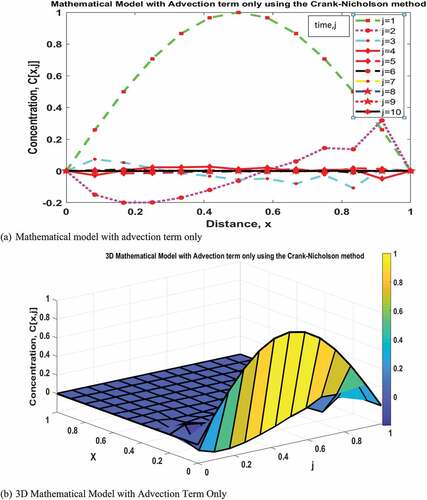
Figure 2. Solutions to the governing equations with diffusion term only using Crank-Nicolson method.

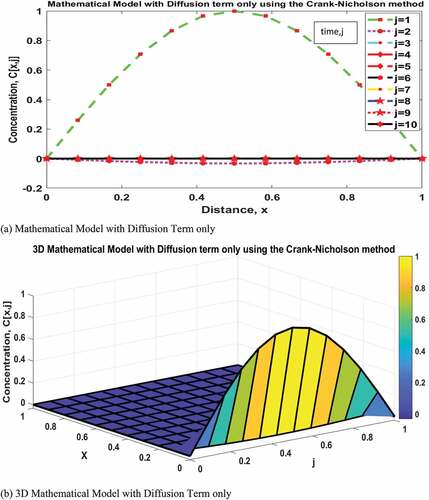
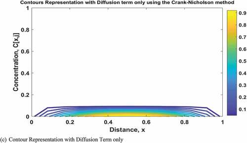
Figure 3. Solutions to the governing equations with advection and diffusion terms using Crank-Nicolson method.

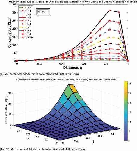
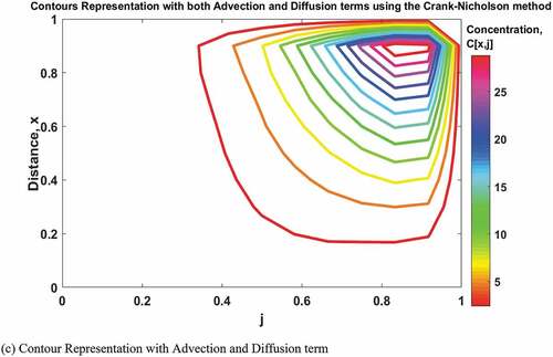
There is a similar trend observed in the solutions to the developed governing equations for indoor-outdoor exchange of air pollutants from electric power generators servicing buildings when advection term and diffusion term were considered separately. The concentration profiles for advection term only and diffusion term only show that the concentrations of air pollutants decrease with time and remains constant at a point. The direct relationship between the concentrations and time is consistent with the results of the solution to the advection of a sudden release of pollutants into a channel as reported by Zoppou and Knight (1997). Both solutions show a non–uniform distribution of air pollutants which could have significant effect on indoor air quality provided it is not affected by other factors such as high wind speed of the outdoor environment. The contrast noticed at the constant point could be a function of the assumption of the constant variables considered, difference in the mathematical scheme used and consideration of rate of decay of pollutant leaving a building section (K). However, when advection and diffusion terms were considered, an inverse relationship between concentration and time which shows the profile attenuates can be seen in the solution to the mathematical model. The report by Ahmed (2012), on the study of “numerical solution to advection-diffusion equation at constant and variable coefficients” showed a similar trend though a developed scheme which combines the Siemieniuch-Gradwell time-difference formula and the Dehghan’s approximation for spatial variable was used. Generally, the results show that the air pollutants entering the building are spreading with varying diffusion term and /or advection term with respect to time and space which is similar to the conclusion of Andallah and Khatun (2020).

5. Conclusion

Generally, mathematical models are used to estimate the impact of the concentration of air pollutants on people. Governing equations with solution of concentrations varying with time and space can be established for air emissions from outdoor electric power generators operated near buildings and their effects indoor air quality. These governing equations can be developed with consideration of advection term only, diffusion term only or both terms using the mass balance approach. The Crank-Nilcoson scheme works well in obtaining numerical solutions when studying the advection and/or diffusion equations. The concentrations of air pollutants decrease with time and remains constant at a point when the concentration profiles of advection term only and diffusion term only were considered but differs when both terms were considered together. Further work can be done on stability conditions of the scheme.

Research activities

• The research work in this paper is related to a Ph.D work carried out by the first author on the “modeling of indoor-outdoor air exchange for safe location of electric power generators servicing buildings”.

• The research activities with regards to this paper include: review of various articles on developing advection-diffusion models with special interest in those related to dispersion of air pollutants into buildings from point sources and their effects on indoor air quality; review of articles on solving of advection-diffusion equations; development of governing equations; using of Crank-Nicolson implicit finite difference techniques: using of Matrix Laboratory (MATLAB) software for solving the developed advection-diffusion equations and result analysis.

Application

• This work can be related to research work done on developing advection-diffusion models to predict concentrations or dispersion of air pollutants or chemically reactive materials released from area sources, line sources and other point sources near buildings.

• It can be extended to the case of numerical solution for 2-Dimensional advection-diffusion problems.

Disclosure statement

No potential conflict of interest was reported by the author(s).

Additional information

Funding

The authors received no direct funding for this research.

References

- Agarwal, M., & Tandon, A. (2009). Modelling of the urban heat island in the form of mesoscale wind and of its effect on air pollution dispersal. Applied Mathematical Modelling, 34, 2520–19.
- Ahmed, S. G. (2012). A numerical algorithm for solving advection-diffusion equation with constant and variable coefficients. Open Numerical Methods Journal, 4(1), 1–7. https://doi.org/10.2174/1876389801204010001
- Andallah, L. S., & Khatun, M. R. (2020). Numerical solution of advection-diffusion equation using finite difference schemes. Bangladesh Journal of Scientific and Industrial Research, 55(1), 15–22. https://doi.org/10.3329/bjsir.v55i1.46728
- Anggarani, B., Wibowo, P., & Aditama, F. (2019). Air dispersion modelling for emission mitigation of power plant technology. The 2019 International Conference on Mining and Environmental Technology, IOP Conference Series: Earth and Environmental Science; 413.
- Crank, J. (1975). The Mathematics of Diffusion 2nd ed. Clarendon Press Oxford.
- Cuson, D. M., & Mingham, C. G. (2010). Introductory to finite difference methods for PDEs. Ventus Publishing ApS.
- Davis, M. L., & Cornwell, D. A. (2013). Introduction to environmental engineering 5th ed., McGraw Hill Companies.
- Dehghan, M. (2004). Numerical solution of the three-dimensional advection-diffusion equation. Applied Mathematics and Computation, 150(1), 5–19. https://doi.org/10.1016/S0096-3003(03)00193-0
- Duffy, D. J. (2004). A critique of the crank nilcoson scheme strenths and weaknesses for financial instrument pricing. Datasim Component Technology BV. Wilmott Magazine: 69–76.
- Freijar, J. I. & Bloeman, H. J. (2000). Modeling relationships between indoor and outdoor air quality. Journal of Air and Waste Management Association, 50(2), 292–300. https://doi.org/10.1080/10473289.2000.10464007
- Hoffman, J. D. (1992). Numerical methods for engineering and scientist. McGraw-Hill Inc.62 M. Thongmoon & R. McKibbin.
- International Energy Agency. (2011). Key world energy statistics. Available: https://www.iea.org/reports/key-world-energy-statistics-2020 ( accessed on 12 April 2021).
- Margulis, P. S., & Acharya, M. (2016). Addressing indoor air pollution in Africa: key to improving household health. http://www.unep.org/urban_environment/PDFs/IAPAfrica.pdf. Accessed on 1st of September 2012
- Milner, J. T., Dimitroulopoulou, C., & ApSimon, H. M. (2015). Indoor concentrations in buildings from sources outdoors. Air Quality Management Liason Committee, 1–82.
- Narayanachari, K. L., Suresha, C. M., Siddalinga, P. M., & Pandurangappa, C. (2014). Time dependent advection diffusion model of air pollutants with removal mechanisms. International Journal of Environmental Science, 5, 34–50.
- Oladipupo, O. (2017). Respiratory disease associated with community air pollution and a steel mill, Utah Valley. American Journal of Public Health, 79(5), 63–628.
- Omole, D. O., & Ndambuki, J. M. (2014). Sustainable Living in Africa: Case of Water, Sanitation. Air Pollution & Energy, Sustainability, 6(8), 5187–5202.
- Omole, D. O., & Ndambuki, J. M. (2015). Nigeria’s legal instruments for land and water use: Implications for national development. In E. Osabuohien (Ed.), In-Country determinants and implications of foreign land acquisitions. Hershey, PA, USA: IGI GLOBAL. (pp. 354–373).
- Stockie, J. M. 2010. The mathematics of atmospheric dispersion modelling. Department of Mathematics, Simon Fraser University: 8888 University Drive, Burnaby, BC, V5A 1S6, Canada .
- Thongmoon, M., & McKibbin, R. (2006). A comparison of some numerical methods for advection-diffusion equation. Research Letters in the Information and Mathematical Sciences, 10, 49–62.
- Thongmoon, M., McKibbin, R., Tangmanee, S. (2007). Numerical solution of a 3-D advection-dispersion model for pollutant transport. Thai Journal of Mathematics, 5(1), 91–108.
- Ulfah, S., Bekoe, C., & Owusu, B. A. (2015). Advection – diffusion model with time dependent for air pollutants distribution in unstable atmospheric condition. Indonesian Journal of Statistics, 20, 2.
- Zoppou, C., & Knight, J. H. (1997). Analytical solutions for advection and advection – diffusion equations with spatially variable coeffiecients. Journal of Hydraulic Engineering, 123(2), 144–147. https://doi.org/10.1061/(ASCE)0733-9429(1997)123:2(144)