Mapping Ethiopian ionosphere using ground-based GPS TEC

Abstract

The objective of this paper is to map regional ionospheric Total Electron Content (vTEC) using Global Positioning System (GPS) data from 10 different GPS receiver sites in Ethiopia, to capture ionospheric phenomena (such as storm effect, Equatorial Ionization Anomaly (EIA) distribution) and to see the hourly evolution of the ionosphere for a single stormy day. GPS based TEC data acquired on 17 March 2013 was used for diurnal and anomaly observations and 17 March 2015 storm-day (storm intensity, Dst = −222nT) data was used for storm-time vTEC mapping. For regional ionosphere characterization, we converted slant TEC (sTEC) to equivalent vTEC. This is done by applying the ionospheric thin shell model. For smooth latitude and longitude boundary interpolation inverse distance weighted (IDW) interpolation technique was used. The map was produced with spatial resolution of ${0.8}^0$ by ${0.8}^0$ latitude and longitude, respectively. The result shows significant diurnal dependence of TEC. It also exhibits an equatorial ionospheric anomaly, characterized by minimum vTEC associated to lower latitudes and maximum vTEC over the higher latitude in the region. We noted that the equatorial anomaly distribution is pronounced during several of the early afternoon hours (13:00Lt, 14:00 LT and 15:00LT). The maps showed the enhancement of vTEC up to 85TECU during 17 March 2015 storm compared to the depletion up to 40TECU on 19 March 2015.

Keywords:

• sTEC
• vTEC
• ionospheric mapping
• geomagnetic storm

1. Introduction

The ionosphere is a partially ionized medium found at about 60 –1000 km altitude in the thermosphere-upper part of the terrestrial atmosphere. Its presence was speculated by many but confirmed in 1924 by Appleton and Barret using ionosondes. It is characterized by free electrons and ions as a result of photoionization and impact ionization of its neutral constituents.

It has a very important implication in radio communication without satellite involvement in spite of the curvature of the earth. On the other hand, it also affects satellite navigation as a result of its dispersing effect on electromagnetic waves. It leads to a time delay of the radio signals, for instance, GPS satellite signals get delayed in the ionosphere. This is due to the interaction of the signals with the free electrons (Gustavsson & Eliasson, 2008). The ionospheric delay is found out to be the limiting factor in high-accuracy positioning systems (Rovira-Garcia et al., 2015). Global ionospheric vTEC maps are thus important for generating real-time global vTEC maps as they can be used for short-term prediction (Orús Pérez et al., 2010).

The effect of the ionosphere on radio signals depends on the signal frequency (Keith Hargreaves, 1979) and the number of electrons present along the path of the signal. Moreover, the electron density irregularities have also a profound effect on the amplitude and phase of the signals, though it is not our interest here.

TEC is the total number of electrons present along a path of a radio signal between a satellite and receiver. The parameter of the ionosphere that produces most of the effects on radio signals is TEC (Kersley et al., 2004; Ya’acob et al., 2008). Radio waves are affected by the presence of electrons and the electron density fluctuations in the path of propagation (Fejer, 1960). The more electrons in the path of the radio wave, the more the radio signal will be affected. For ground to satellite communication and satellite navigation, TEC is a good parameter to monitor for possible space weather impacts.

TEC is measured in electrons per square meter. By convention, 1TEC Unit (TECU) = ${10}^{16}electrons/m^2$. Vertical TEC values in Earth’s ionosphere can range from a few to several hundred TECU. TEC in the ionosphere is modified by changing solar Extreme Ultraviolet radiation, geomagnetic storms, and the atmospheric waves that propagate up from the lower atmosphere. The dominant mechanisms accountable for the high variability of TEC at the equatorial and low latitude ionosphere are the EIA, equatorial electrojet (EEJ), Equatorial Spread F (ESF), and geomagnetic storms (Lo Ciraolo et al., 2007, 2; Bagiya et al., 2009, 6; Vishal Chauhan & Singh, 2011; Bolaji et al., 2012). TEC trends do correlate well with the solar activity indices such as the sunspot number and F 10.7 indices as shown by Bagiya et al. (2009); Gupta & Singh (2000); Praveen Galav et al. (2010). The seasonal variation in TEC is similar to the seasonal variation in the EIA formations (Asmare Tariku, 2015; Bertillas Amabayo et al., 2014; Olwendo et al., 2012). The temporal and spatial variability of TEC at the equatorial and low latitudes depends on the time of the day, season, and solar activity (Kumar & Singh, 2009; Praveen Galav et al., 2010).

The propagation of radio waves is affected by the ionosphere. The velocity of radio waves changes when the signal passes through the electrons in the ionosphere. The total delay suffered by a radio wave propagating through the ionosphere depends both on the frequency of the radio wave and the TEC between the transmitter and the receiver. At some frequencies, the radio waves pass through the ionosphere. At other frequencies, the waves are reflected by the ionosphere. TEC is the measure of electrons per square meter over a length of a column from a satellite at about 20,200 km altitude (considering only a satellite overhead otherwise the distance is greater than 20,200 km) to a receiver on the surface of the earth (Bust & Mitchell, 2008). The nominal range is ${10}^{16}electrons/m^2$ to ${10}^{18}electrons/m^2$ (1TECU to 100TECU) with minima and maxima occurring at midnight and mid afternoon approximately (Ya’acob et al., 2008).

The knowledge of the nature of temporal and spatial variations in TEC is very useful for users of satellite-based navigation systems as well as any kind of radio communication using skywave. Changes of any magnitude in TEC are a serious concern, particularly at low and equatorial latitudes due to the chaotic nature of the ionosphere in this region (Akala et al., 2010; Akala & Doherty, 2012; Akala et al., 2011). GPS-based applications are widely used (Hofmann-Wellenhof et al., 2001) and they encounter the largest errors as the result of electron density irregularities in the path of the satellite signal (Klobuchar, 1986). Therefore, variations in the GPS-TEC have been extensively studied (Maruyama et al., 2004). The objective of this paper is to map regional ionospheric vTEC using data acquired by GPS stations in Ethiopia, to capture any ionospheric phenomena (such as storm effect, EIA distribution) and to see the hourly evolution of the ionosphere for a single stormy day. We have produced the map with a spatial resolution of ${0.8}^0$ by ${0.8}^0$ latitude and longitude, respectively, and an hour temporal resolution for the day 17 March 2013. Besides, the storm-time mapping was done for 17 March 2015 (St. Patrick’s Day). Though few attempts were done in imaging Ethiopian ionosphere (e.g. (Kindie Mengist et al., 2015)), such ionospheric mapping is new in Ethiopian context. The current mapping incorporates the temporal and storm-time analysis which previous studies did not report (Kassa et al., 2012; Kindie Mengist et al., 2015). Moreover, we used more ground based GPS receivers (10) and the data is original.

2. Data and methodology

2.1. Data

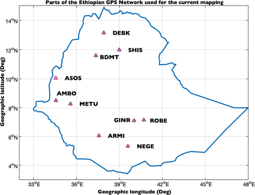
For this paper, GPS-based TEC data acquired on 17 March 2013 by 10 stations scattered over Ethiopia was used. The storm-time analysis was for 17 March 2015 storm. We selected these days for two reasons:

• All the stations under study have collected complete set of data.

• There was severe storm on 17 March 2015, which is appropriate to see the storm effect on TEC. Unfortunately, only seven of the 10 stations have collected complete set of data during 17 March 2015.

The Data was accessed through internet from UNAVCO archive (http://www.unavco.org/). Figure 1 displays geographic locations of the GPS receivers used in this study.

Hourly values of interplanetary parameters such as the y-component of the Interplanetary Electric Field (IEF) of Ey, the Z-component of Interplanetary Magnetic Field (IMF) of Bz, and geomagnetic storm parameters such the longitudinal Symetric Horizontal component disturbance index (Sym-H) for 16–20 March 2015 data and Disturbed time index (Dst) for 16–19 March 2015 data are obtained from https://omniweb.gsfc.nasa.gov/ archive. The Sym-H and Dst index characterize the storm intensity.

Figure 1. Geographical locations of GPS receivers used in the study.

2.2. Methodology

2.2.1. TEC extraction from dual frequency GPS receiver

The receivers at GPS stations record signals transmitted at two L-band frequencies namely, $f_1$ at 1575.42 MHz, and $f_2$ at 1227.60 MHz. The time delay which occurs while these signals are propagating through the ionosphere are converted to pseudo-ranges and recorded as $P_1$ and $P_2$ signals. The carrier phase delay measurements on the $f_1$ and $f_2$ coherent frequencies are also recorded as $L_1$ and $L_2$, respectively. The delayed and phase shifted signals are recorded in a special format called Receiver Independent Exchange Format (RINEX). The time delay of signals are converted to pseudo-range values and the phase shifts are recorded as phase delays in the receivers (Lo Ciraolo et al., 2007; Klobuchar, 1986; Mannucci et al., 1998) . The standard model for pseudo-range recordings for two frequencies $f_1$ and $f_2$ are as follows:

(1) $\begin{array}{cc}{P}_{1,u}^m=& {\rho }_u^m+c(\delta t_u-\delta t^m)+d_{trop,u}^m+d_{ion1,u}^m\\ \hspace{0.17em}& +c({\epsilon }_1^m+{\epsilon }_{1,u})\end{array}$(1)

(2) $\begin{array}{cc}{P}_{2,u}^m=& {\rho }_u^m+c(\delta t_u-\delta t^m)+d_{trop,u}^m+d_{ion2,u}^m\\ \hspace{0.17em}& +c({\epsilon }_2^m+{\epsilon }_{2,u}),\end{array}$(2)

where the subscript $u$ denotes the receiver station index; the subscript $m$ denotes the satellite index. $\rho$ is the actual range between satellite and receiver, $\delta t_u$ and $\delta t^m$ are the clock errors for the receiver and satellite, respectively.

$d_{trop}$ and $d_{ion}$ are the troposphere and ionosphere group delays, respectively. ${\epsilon }^m$ and ${\epsilon }_u$ are the frequency-dependent satellite and receiver biases. The model for GPS recordings also include antenna pattern and noise errors. Since those are assumed to be the same for both frequencies, usually they are not spelled out in the model equation for TEC. $c$ is the speed of light in vacuum.

The difference of Equations (1)(1) $\begin{array}{cc}{P}_{1,u}^m=& {\rho }_u^m+c(\delta t_u-\delta t^m)+d_{trop,u}^m+d_{ion1,u}^m\\ \hspace{0.17em}& +c({\epsilon }_1^m+{\epsilon }_{1,u})\end{array}$(1) and (2(2) $\begin{array}{cc}{P}_{2,u}^m=& {\rho }_u^m+c(\delta t_u-\delta t^m)+d_{trop,u}^m+d_{ion2,u}^m\\ \hspace{0.17em}& +c({\epsilon }_2^m+{\epsilon }_{2,u}),\end{array}$(2) ) is called the geometry free linear combination of pseudo-range because the actual range $\rho$ is eliminated as

(3) $\begin{array}{cc}{P}_{4,u}^m=& P_{2,u}^m-P_{1,u}^m=d_{ion2,u}^m-d_{ion1,u}^m\\ \hspace{0.17em}& +c({\epsilon }_2^m-{\epsilon }_1^m)+c({\epsilon }_{2,u}-{\epsilon }_{1,u}).\end{array}$(3)

The tropospheric contribution $d_{trop,u}^m$ in Equations (1)(1) $\begin{array}{cc}{P}_{1,u}^m=& {\rho }_u^m+c(\delta t_u-\delta t^m)+d_{trop,u}^m+d_{ion1,u}^m\\ \hspace{0.17em}& +c({\epsilon }_1^m+{\epsilon }_{1,u})\end{array}$(1) and (2(2) $\begin{array}{cc}{P}_{2,u}^m=& {\rho }_u^m+c(\delta t_u-\delta t^m)+d_{trop,u}^m+d_{ion2,u}^m\\ \hspace{0.17em}& +c({\epsilon }_2^m+{\epsilon }_{2,u}),\end{array}$(2) ) and any other source of error are also eliminated since they are not a function of frequency. Using satellite and receiver biases for $f_1$ and $f_2$ frequency signals, inter-frequency or differential code biases (DCBs) are defined for the satellite and receiver as follows:

(4) $DC{B}^m={\epsilon }_1^m-{\epsilon }_2^m$(4)

(5) $DC{B}_u={\epsilon }_{1,u}-{\epsilon }_{2,u},$(5)

where $DC{B}^m$ and $DC{B}_u$ are the differential code biases for the satellite and receiver, respectively.

Similar equation can be written for phase delay observations $L_{1,u}^m$ and $L_{2,u}^m$ as:

(6) $\begin{array}{cc}{L}_{1,u}^m=& {\lambda }_1{\mathrm{\Phi }}_{1,u}^m={\rho }_u^m+c(\delta t_u-\delta t^m)\\ \hspace{0.17em}& +{\lambda }_1{\mathrm{\Phi }}_{ion1,u}^m+{\lambda }_1{\mathrm{\Phi }}_{trop,u}^m-c({\epsilon }_1^m+{\epsilon }_{1,u})+{\lambda }_1{N}_1^m\end{array}$(6)

(7) $\begin{array}{cc}{L}_{2,u}^m=& {\lambda }_2{\mathrm{\Phi }}_{2,u}^m={\rho }_u^m+c(\delta t_u-\delta t^m)\\ \hspace{0.17em}& +{\lambda }_2{\mathrm{\Phi }}_{ion2,u}^m+{\lambda }_2{\mathrm{\Phi }}_{trop,u}^m-c({\epsilon }_2^m+{\epsilon }_{2,u})+{\lambda }_2{N}_2^m,\end{array}$(7)

where ${\lambda }_1$ and ${\lambda }_2$ are the wavelengths corresponding to $f_1$ and $f_2$ frequencies, ${\mathrm{\Phi }}_{ion1,u}^m$ and ${\mathrm{\Phi }}_{ion2,u}^m$ are the ionospheric phase delays corresponding to $f_1$ and $f_2$ frequencies, respectively. $N_1^m$ and $N_2^m$ denote the initial phase ambiguity corresponding to $f_1$ and $f_2$ frequencies, respectively, for the $m^{th}$ satellite. Finally, ${\mathrm{\Phi }}_{trop,u}^m$ is the phase delay due to troposphere.

The difference of Equations (6)(6) $\begin{array}{cc}{L}_{1,u}^m=& {\lambda }_1{\mathrm{\Phi }}_{1,u}^m={\rho }_u^m+c(\delta t_u-\delta t^m)\\ \hspace{0.17em}& +{\lambda }_1{\mathrm{\Phi }}_{ion1,u}^m+{\lambda }_1{\mathrm{\Phi }}_{trop,u}^m-c({\epsilon }_1^m+{\epsilon }_{1,u})+{\lambda }_1{N}_1^m\end{array}$(6) and (7(7) $\begin{array}{cc}{L}_{2,u}^m=& {\lambda }_2{\mathrm{\Phi }}_{2,u}^m={\rho }_u^m+c(\delta t_u-\delta t^m)\\ \hspace{0.17em}& +{\lambda }_2{\mathrm{\Phi }}_{ion2,u}^m+{\lambda }_2{\mathrm{\Phi }}_{trop,u}^m-c({\epsilon }_2^m+{\epsilon }_{2,u})+{\lambda }_2{N}_2^m,\end{array}$(7) ) is called the geometry free linear combinations of phase delay and is given by

(8) $\begin{array}{cc}{L}_{4,u}^m=& {\lambda }_1{\mathrm{\Phi }}_{1,u}^m-{\lambda }_2{\mathrm{\Phi }}_{2,u}^m={\lambda }_1{\mathrm{\Phi }}_{ion1,u}^m-{\lambda }_2{\mathrm{\Phi }}_{ion2,u}^m\\ \hspace{0.17em}& -c(DC{B}^m)-c(DC{B}_u)+\mathrm{\Delta }{N}^m,\end{array}$(8)

where $\mathrm{\Delta }{N}^m$ in Equation (8)(8) $\begin{array}{cc}{L}_{4,u}^m=& {\lambda }_1{\mathrm{\Phi }}_{1,u}^m-{\lambda }_2{\mathrm{\Phi }}_{2,u}^m={\lambda }_1{\mathrm{\Phi }}_{ion1,u}^m-{\lambda }_2{\mathrm{\Phi }}_{ion2,u}^m\\ \hspace{0.17em}& -c(DC{B}^m)-c(DC{B}_u)+\mathrm{\Delta }{N}^m,\end{array}$(8) is defined as

(9) $\mathrm{\Delta }{N}^m={\lambda }_1{N}_1^m-{\lambda }_2{N}_2^m.$(9)

Using the approximation given by Lo Ciraolo et al. (2007); Klobuchar (1986); Mannucci et al. (1998)

(10) $d_{ion,u}^m=-{\mathrm{\Phi }}_{1,u}^m\frac{c}{f}\approx A\frac{sTE{C}_u^m}{f^2},$(10)

where $A=40.3m^3/s^2$ and $sTE{C}_u^m$ denotes the total electron content on the slant ray path combining the receiver $u$ and the satellite $m$. Using Eq. (10)(10) $d_{ion,u}^m=-{\mathrm{\Phi }}_{1,u}^m\frac{c}{f}\approx A\frac{sTE{C}_u^m}{f^2},$(10) in Eq. (3)(3) $\begin{array}{cc}{P}_{4,u}^m=& P_{2,u}^m-P_{1,u}^m=d_{ion2,u}^m-d_{ion1,u}^m\\ \hspace{0.17em}& +c({\epsilon }_2^m-{\epsilon }_1^m)+c({\epsilon }_{2,u}-{\epsilon }_{1,u}).\end{array}$(3) and (8(8) $\begin{array}{cc}{L}_{4,u}^m=& {\lambda }_1{\mathrm{\Phi }}_{1,u}^m-{\lambda }_2{\mathrm{\Phi }}_{2,u}^m={\lambda }_1{\mathrm{\Phi }}_{ion1,u}^m-{\lambda }_2{\mathrm{\Phi }}_{ion2,u}^m\\ \hspace{0.17em}& -c(DC{B}^m)-c(DC{B}_u)+\mathrm{\Delta }{N}^m,\end{array}$(8) ), the following expressions for the geometry free combinations are obtained

(11) $P_{4,u}^m=A\left(\frac{f_1^2-f_2^2}{f_1^2{f}_2^2}\right)sTE{C}_u^m-c(DC{B}^m+DC{B}_u)$(11)

(12) $L_{4,u}^m=A\left(\frac{f_1^2-f_2^2}{f_1^2{f}_2^2}\right)sTE{C}_u^m-c(DC{B}^m+DC{B}_u)+\mathrm{\Delta }{N}^m.$(12)

For a selected measurement time, slant Ray Total Electron Content (sTEC) can be calculated using either pseudo-range or carrier phase data from each satellite. sTEC calculated from Eq. (11)(11) $P_{4,u}^m=A\left(\frac{f_1^2-f_2^2}{f_1^2{f}_2^2}\right)sTE{C}_u^m-c(DC{B}^m+DC{B}_u)$(11) is noisy and open to multipath effects:

(13) $sTE{C}_u^m(n)=\frac{1}{A}\left(\frac{f_1^2{f}_2^2}{f_1^2-f_2^2}\right)\left[P_{4,u}^m(n)+c(DC{B}^m+DC{B}_u)\right],$(13)

where $N$ is the number of sTEC observations, the index $n$ denotes the time sample, and $1\le n\le N$.

In order to solve $sTEC$ from equation (12)(12) $L_{4,u}^m=A\left(\frac{f_1^2-f_2^2}{f_1^2{f}_2^2}\right)sTE{C}_u^m-c(DC{B}^m+DC{B}_u)+\mathrm{\Delta }{N}^m.$(12) , the initial ambiguity $\mathrm{\Delta }{N}^m$ needs to be resolved. In the works of (Lo Ciraolo et al., 2007; Klobuchar, 1986; Mannucci et al., 1998), the following baseline method is used: First, a baseline, $B$, for each connected arc is obtained by differentiating pseudorange and phase measurements as

(14) $B=\frac{1}{N_{me}}\sum _{n_{me}=1}^{N_{me}}\left(P_{4,u}^m(n_{me})-L_{4,u}^m(n_{me})\right),$(14)

where $N_{me}$ is the number of measurements in a connected phase arc. Then the slant TEC can be computed by inserting $B$ into the phase equation (12)(12) $L_{4,u}^m=A\left(\frac{f_1^2-f_2^2}{f_1^2{f}_2^2}\right)sTE{C}_u^m-c(DC{B}^m+DC{B}_u)+\mathrm{\Delta }{N}^m.$(12) and sTEC can be extracted as

(15) $\begin{array}{cc}sTE{C}_u^m(n)& =\frac{1}{A}\left(\frac{f_1^2{f}_2^2}{f_1^2-f_2^2}\right)(B+L_{4,u}^m(n)\\ \hspace{0.17em}& +c(DC{B}_u+DC{B}^m)).\end{array}$(15)

In the above equations, $u$ and $m$ denote the receiver and satellite id’s, respectively, $n$ is the measurement time. $L_4$ is the geometry free linear combination of carrier phase data and $B$ is the baseline value that is defined in equation (14)(14) $B=\frac{1}{N_{me}}\sum _{n_{me}=1}^{N_{me}}\left(P_{4,u}^m(n_{me})-L_{4,u}^m(n_{me})\right),$(14) . $DC{B}_u$ and $DC{B}^m$ are the receiver and satellite differential code biases, respectively. Each cycle slip or phase disconnection starts another baseline calculation. Once the slant TEC is computed, the vertical TEC, vTEC, can be obtained using thin shell approximation of Single Layer Ionosphere Model (SLIM) as

(16) $vTE{C}_u^m(n)=\frac{sTE{C}_u^m(n)}{M({\epsilon }_m(n))},$(16)

where $M({\epsilon }_m(n))={\left[1-{\left(\frac{Rcos{\epsilon }_m(n)}{R+h}\right)}^2\right]}^{\frac{-1}{2}}$ is called the mapping function and ${\epsilon }_m$ is the satellite eleva-tion angle. $R$ is the earth radius of 6, 378.137 km and $h$ is the ionospheric shell height of 350 km.

The TEC data used was calibrated at an hour interval by removing the data received below elevation angle ${40}^0$. The station based hourly average data was calculated by taking the mean of TEC measured by satellites tracked over the hour interval with specified elevation. Then, the single valued station data was scatter plotted for each hour. For smooth latitude and longitude boundary interpolation inverse distance weighted (IDW) interpolation technique is used. The IDW interpolation is a method that imposes the condition that the estimated value of a point is influenced more by nearby known points than by those farther away. This makes the IDW method more preferable to TEC mapping over a region.

The generalized equation used for IDW interpolation, as used in (Kindie Mengist et al., 2015), is given as

(17) $F_0=\frac{{\sum }_{i=1}^s\frac{F_i}{d_i}}{{\mathrm{\Sigma }}_{i=1}^s\frac{1}{d_i^k}}$(17)

where, $F_0$ is the estimated value at point $0$, $F_i$ is the $F$ value at known point $i$, $d_i$ is the distance between point i and point $0$, $s$ is the number of known points used in the estimation, and k is the specified power. Using the hourly average vTEC values with their corresponding station locations as $F_i$, we applied the IDW interpolation scheme to calculate the vTEC values within ${0.8}^0$ by ${0.8}^0$ latitude and longitude grid.

3. Result and discussion

3.1. vTEC diurnal variations

Figures 2–4 illustrate how vTEC values vary on a typical day. They show vTEC maps of the Ethiopian ionosphere in hourly intervals from 01:00UT 24:00 UT on 17 March 2013.

Figure 2 depicts that vTEC values were decreasing for 01:00UT and 02:00UT showing the minimum values during 03:00 UT ad 04:00UT and increasing again from 05:00UT onwards. In Figure 3, we can also observe the increase in vTEC values until we reach 15:00 UT where the maximum value of the day was attained and start decreasing for the rest of the hours. The maps in Figure 4 show vTEC values to be fairly constant for three hours and then start decreasing as time goes on.

Figure 2. vTEC maps of Ethiopia from 01:00–09:00 UT on 17 March 2013.

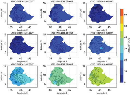
Looking at the maps generated at 07:00 UT of Figure 2 to the maps generated at 18:00 UT of Figure 4, we can understand that the vTEC values are higher in the afternoon than during other times of the day. Though it drops a little bit after 17:00 UT (20:00LT), vTEC is higher in the afternoon hours until just past midnight as displayed by Figure 4.

Figure 3. vTEC maps of Ethiopia from 10:00–18:00 UT on 17 March 2013.

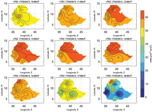
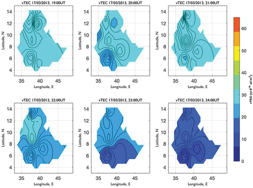
Figure 2 shows that during the morning hours of the day, beginning at 06:00 UT, late after sun rise the vTEC values slowly increase from the night time value. During the evening hours, early after sunset the vTEC values therefore gradually reduce, which can be seen in the maps generated at 18:00 UT the last map of Figure 4 and generated at 19:00 UT the first map of Figure 4. After sunset, vTEC values were expected to rapidly decrease due to the electron recombination process in the absence of ionizing solar UV but still, the vTEC values remain significantly higher than the morning vTEC values as shown in Figure 4. The overall map shows that the ionization of the day was kept high for the whole afternoon.

Figure 4. vTEC maps of Ethiopia from 19:00–24:00 UT on 17 March 2013.

3.2. Equatorial Ionization Anomaly (EIA)

EIA is the the unusual accumulation of plasma $\pm {10}^0$ to $\pm {20}^0$ the geographic equator. It is mainly observed from 09:00UT- 16:00UT (11:00 LT-19:00 LT) hours. It is formed not from the local photo ionization of plasma at the crests but mainly from the removal of plasma from around the equator by the upward ExB drift where the crests are within approximately $\pm {20}^0$ magnetic latitude though the accumulations reduce with increasing latitude and become zero by approximately $\pm {25}^0$ (Balan et al., 2018; Fejer, 1960; Keith Hargreaves, 1979).

Figure 5. Latitudinal variations of vTEC from 01:00–08:00 UT on 17 March 2013 over Ethiopia.

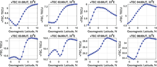
Figures 5–7 depict the latitudinal variations of vTEC in the Ethiopian sector at ${33}^{0}E$ longitude.The latitudinal plots are done at ${33}^{0}E$ longitude which can be considered as the the beginning of longitude of Ethiopia. To clearly see the appearance of equatorial ionization anomaly, we have converted geographic latitudes to geomagnetic coordinates. From these Figs., it can be deduced that the maximum TEC values observed during, before and after the noon hours in the range of $-5^0$ -${10}^0$ latitude is the result of EIA.

Figure 6. Latitudinal variations of vTEC from 09:00–16:00 UT on 17 March 2013 over Ethiopia.

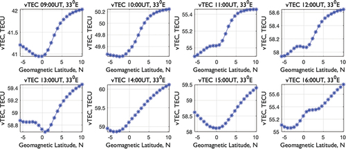
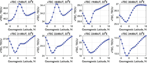
Figure 7. Latitudinal variations of vTEC from 17:00–24:00 UT on 17 March 2013 over Ethiopia.

The Maps for 09:00UT- 16:00UT (11:00 LT-19:00LT) hours of the day show that the vTEC values increase with latitude increase in the region, which may assure the occurrence of EIA distribution within Ethiopian ionosphere for the day considered. This notion is supported by (Kindie Mengist et al., 2015) as the paper points out that in the East African region vTEC varies diurnally, with a peak in the late afternoon $t\le$ 17:00 LT), due to the equatorial ionospheric anomaly.

The variability in TEC has positive dependence on solar activity in spite of the fact that the quiet days and disturb days TEC behave differently in such a way that variation in TEC is maximum for disturbed days and minimum for quiet days (Maski & Vijay, 2016). Figures 2 to 7 display vTEC maps as well as latitudinal variations of vTEC for 17 March 2013. From the figures it is clearly distinguishable that the maximum vTEC for the day happens later than the expected hour (midday, 12:00UT) and stayed longer.

3.3. St. Patrick’s Day storm of 17 March 2015

The St. Patrick’s Day storm of 17 March 2015 is, so far, the strongest geomagnetic storm of the current solar cycle 24. As a result, it has garnered considerable interest in the scientific community. There have been a number of studies which investigated the ionospheric effects of this particular storm. Studies by Astafyeva et al. (2015); Chin-Chun et al. (2016) have reported the global variation of plasma bubble occurrence during the St. Patrick’s Day storm. In the current study, we have investigated the effect of the 17 March 2015 storm in the Ethiopian longitudinal sector and how it enhanced the ionospheric vTEC inferred from vTEC maps.

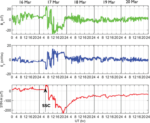
Figure 8. Diurnal variation of: IMF Bz component (top panel), IEF Ey component (middle panel) and $\mathit{S}y{m}_H$ index (bottom panel) from 16 to 20 March 2015.

3.3.1. Event description

As we can see from the bottom panel of Figure 8, the arrival of Shock at the Earth produced a sudden storm commencement (SSC) at 04:45 UT. The value of Dst started decreasing right after the IMF turned south-ward. The storm intensified (Dst dropped to −80 nT at $\sim$ 10:00 UT) during the passage of the sheath (a region between the shock and the driver of the shock). Later, the storm recovered slightly (i.e., Dst dropped to $\sim$ −50 nT), shortly after the IMF turned northward. A few hours later, the IMF turned southward again due to the strongly negative Bz in the magnetic cloud (MC) and caused the second storm intensification, reaching Dst = −222 nT on 17 March. We conclude that the St. Patrick’s day event (17 March) is a two-step storm. The first step was associated with a southward IMF embedded in the sheath region, whereas the second step was associated with a southward MC field.

3.3.2. Storm-time vTEC maps

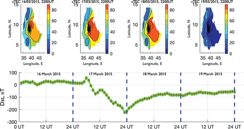
The top panel of Figure 9 depicts the map of vTEC during 16–19 March 2015. The bottom panel of this figure demonstrates the daily variations of Sym-H (16–19 March 2015). The map was done at 22:00 UT at which Sym-H attained its minimum value (−222 nT) on 17 March 2015. During the main phase of 17 March 2015 storm, the vTEC was enhanced to about 85 TECU and starts to decrease on the recovery day, 18 March 2015, and reaches to a minimum value about 40 TECU on 19 March 2015. Surprisingly, the vTEC maps clearly showed the enhancement of vTEC during 17 March 2015 storm compared to the depletion of on 19 March 2015. This report is inline with the analysis given by Astafyeva et al. (2015); Chin-Chun et al. (2016).

Figure 9. Storm-time variations of vTEC on 16–19 March 2015 over Ethiopia.

4. Conclusion

Ionospheric vTEC map for Ethiopia on 17 March 2013 has been constructed to study the diurnal variations in the equatorial ionosphere using ground- based GPS data. Stormy day was selected to see the effect of storms on the distribution and trend of vTEC and EIA distribution. The following conclusions are drawn from our analysis.

1. The vTEC maps show the diurnal variation in Ethiopian for the day.

2. The map also exhibits an equatorial ionospheric anomaly, characterized by low vTEC associated to lower latitudes and high vTEC over the higher latitude in the region.

3. We noted that the equatorial anomaly distribution is pronounced during several of the early afternoon hours (13:00LT, 14:00LT and 15:00LT). We also noted that the maximum values of vTEC are observed during these hours of the day.

4. In the future we anticipate that this type of TEC map will be improved by including data for different seasons and thus can be used to study the Ethiopian ionosphere.

5. Surprisingly, the vTEC maps clearly showed the enhancement of vTEC up to 85TECU during 17 March 2015 storm compared to the depletion up to 40TECU on 19 March 2015.

Data availability

The data used to support the finding of this study was free access from internet via UNAVCO archive (http://www.unavco.org/) and https://omniweb.gsfc.nasa.gov/

Acknowledgments

We are grateful to Bahir Dar and Wello Universities, Ethiopia for partly support the current work. The authors also appreciate all data providers for realizing the current work.

Disclosure statement

No potential conflict of interest was reported by the author(s).

Additional information

Funding

The authors received no direct funding for this research.

References

- Akala, A. O., & Doherty, P. H. (2012). Statistical distribution of GPS amplitude scintillations. Journal of atmospheric and solar-terrestrial. Physics, 74, 199–13. https://doi.org/10.1029/2011RS004678
- Akala, A. O., Doherty, P. H., Valladares, C. E., Carrano, C. S., & Sheehan, R. (2011). Statistics of GPS scintillations over South America at three levels of solar activity. Radio Science, 46(5), 1–16. https://doi.org/10.1029/2011RS004678
- Akala, A. O., Oyeyemi, E. O., Somoye, E. O., Adeloye, A. B., & Adewale, A. O. (2010). Variability of fof2 in the African equatorial ionosphere. Advances in Space Research, 45(11), 1311–1314. https://doi.org/10.1016/j.asr.2010.01.003
- Asmare Tariku, Y. (2015). Patterns of GPS-tec variation over low-latitude regions (African sector) during the deep solar minimum (2008 to 2009) and solar maximum (2012 to 2013) phases. Earth, Planets and Space, 67(1), 1–9.
- Astafyeva, E., Zakharenkova, I., & Förster, M. (2015). Ionospheric response to the 2015 St. Patrick’s Day storm: A global multi-instrumental overview. Journal of Geophysical Research, 120(10), 9023–9037. https://doi.org/10.1002/2015JA021629
- Bagiya, M. S., Joshi, H. P., Iyer, K. N., Malini Aggarwal, S. R., & Pathan, B. M. (2009). Tec variations during low solar activity period (2005–2007) near the equatorial ionospheric anomaly crest region in India. In Annales Geophysicae (Vol. 27, pp. 1047–1057). Copernicus GmbH.
- Balan, N., Liu, L., & HuiJun, L. (2018). A brief review of equatorial ionization anomaly and ionospheric irregularities. Earth and Planetary Physics, 2(4), 257–275. https://doi.org/10.26464/epp2018025
- Bertillas Amabayo, E., Edward, J., Cilliers, P. J., & Bosco Habarulema, J. (2014). Climatology of ionospheric scintillations and tec trend over the Ugandan region. Advances in Space Research, 53(5), 734–743. https://doi.org/10.1016/j.asr.2013.12.015
- Bolaji, O. S., Adeniyi, J. O., Radicella, S. M., & Doherty, P. H. (2012). Variability of total electron content over an equatorial West African station during low solar activity. Radio Science, 47(1), 1–9. https://doi.org/10.1029/2011RS004812
- Bust, G. S., & Mitchell, C. N. (2008). History, current state, and future directions of ionospheric imaging. Reviews of Geophysics, 46(1). https://doi.org/10.1029/2006RG000212
- Chin-Chun, W., Liou, K., Lepping, R. P., Hutting, L., Plunkett, S., Howard, R. A., & Socker, D. (2016). The first super geo magnetic storm of solar cycle 24:“the st. patrick’s day event (17 march 2015)”. Earth, Planets and Space, 68(1), 1–12. https://doi.org/10.1186/s40623-016-0525-y
- Fejer, J. A. (1960). Scattering of radio waves by an ionized gas in thermal equilibrium. Canadian Journal of Physics, 38(8), 1114–1133. https://doi.org/10.1139/p60-119
- Gupta, J. K., & Singh, L. (2000). Long term ionospheric electron content variations over Delhi. In Annales Geophysicae (Vol. 18, pp. 1635–1644). Copernicus GmbH.
- Gustavsson, B., & Eliasson, B. (2008). Hf radio wave acceleration of ionospheric electrons: Analysis of hf-induced optical enhancements. Journal of Geophysical Research, 113(A8). https://doi.org/10.1029/2007JA012913
- Hofmann-Wellenhof, B., Lichtenegger, H., & Collins, J. (2001). Applications of GPS. In Global positioning system (pp. 319–343). Springer.
- Kassa, T., Damtie, B., & Yizengaw, E. (2012). The response of Ethiopian ionosphere to the magnetic storm of 11 October 2008. Latin-American Journal of Physics Education, 6(2), 322.
- Keith Hargreaves, J. (1979). The upper atmosphere and solar-terrestrial relations-an introduction to the aerospace environment. New York, 12(18), 37–41.
- Kersley, L., Daniel Malan, S. E. P., Cander, L. J. I. L. J. A. N. A. R., Bamford, R. U. T. H. A., Belehaki, A. N. N. A., Leitinger, R. E. I. N. H. A. R. T., Radicella, S. A. N. D. R. O. M., Mitchell, C. A. T. H. R. Y. N. N., & Spencer, P. A. U. L. S. J. (2004). Total electron content-a key parameter in propagation: Measurement and use in ionospheric imaging. Annals of Geophysics, 47(2–3). https://doi.org/10.4401/ag-3286
- Kindie Mengist, C. K., Ha Kim, Y. H., Yeshita, B. D., & Workayehu, A. B. (2015). Mapping the east African ionosphere using ground-based GPS tec measurements. Journal of Astronomy and Space Sciences, 33(1), 29–36. https://doi.org/10.5140/JASS.2016.33.1.29
- Klobuchar, J. A. Design and characteristics of the GPS ionospheric time delay algorithm for single frequency users. In PLANS’86-Position Location and Navigation Symposium, 280–286, 1986.
- Kumar, S., & Singh, A. K. (2009). Variation of ionospheric total electron content in Indian low latitude region of the equatorial anomaly during may 2007–April 2008. Advances in Space Research, 43(10), 1555–1562. https://doi.org/10.1016/j.asr.2009.01.037
- Lo Ciraolo, L., Azpilicueta, F., Brunini, C., Meza, A., & Radicella, S. M. (2007). Calibration errors on experimental slant total electron content (tec) determined with GPS. Journal of Geodesy, 81(2), 111–120. https://doi.org/10.1007/s00190-006-0093-1
- Mannucci, A. J., Wilson, B. D., Yuan, D. N., Ho, C. H., Lindqwister, U. J., & Runge, T. F. (1998). A global mapping technique for GPS-derived ionospheric total electron content measurements. Radio Science, 33(3), 565–582. https://doi.org/10.1029/97RS02707
- Maruyama, T., Guanyi, M., & Nakamura, M. (2004). Signature of tec storm on 6 November 2001 derived from dense GPS receiver network and ionosonde chain over Japan. Journal of Geophysical Research, 109(A10). https://doi.org/10.1029/2004JA010451
- Maski, K., & Vijay, S. K. Variation of variability in tec for quiet and disturbed days at low latitude station Bhopal using GPS, 2016
- Mukherjee, S., Shivalika Sarkar, S., Purohit, P. K., & Gwal, A. K. (2010). Seasonal variation of total electron content at crest of equatorial anomaly station during low solar activity conditions. Advances in Space Research, 46(3), 291–295. https://doi.org/10.1016/j.asr.2010.03.024
- Olwendo, O. J., Baki, P., Mito, C., & Doherty, P. (2012). Characterization of ionospheric GPS total electron content (GPS–tec) in low latitude zone over the Kenyan region during a very low solar activity phase. Journal of Atmospheric and Solar, 84-85, 52–61. https://doi.org/10.1016/j.jastp.2012.06.003
- Orús Pérez, R., Hernández Pajares, M., Miguel Juan Zornoza, J., Sanz Subirana, J., Ángeles Aragón Ángel, M., & García Rigo, A. Real time application of tomion model. In Beacon Satellite Symposium 2010, 2010.
- Praveen Galav, P., Dashora, N., Sharma, S., & Pandey, R. (2010). Characterization of low latitude GPS-tec during very low solar activity phase. Journal of Atmospheric and Solar, 72(17), 1309–1317. https://doi.org/10.1016/j.jastp.2010.09.017
- Rovira-Garcia, A., Miguel Juan, J. M., Sanz, J., & Gonzalez-Casado, G. (2015). A worldwide ionospheric model for fast precise point positioning. IEEE Transactions on Geoscience and Remote Sensing, 53(8), 4596–4604. https://doi.org/10.1109/TGRS.2015.2402598
- Vishal Chauhan, O. P. S., & Singh, B. Diurnal and seasonal variation of GPS-tec during a low solar activity period as observed at a low latitude station Agra. 94.20. dv; 96.60. qd, 2011.
- Ya’acob, N., Abdullah, M., & Ismail, M. (2008). Determination of GPS total electron content using single layer model (SLM) ionospheric mapping function. International Journal of Computer Science and Network Security, 8(9), 154–160.