Performance evaluation of sand dams as a rural rainwater conservation and domestic water supply technology in East-African drylands, a case-study from South-Eastern Kenya

Abstract

Sand dams (SDs) are rainwater harvesting methods in East-African drylands for rural water supplies and small-scale irrigation practices. However, little information exists on their ability to maintain the harvested water in the right quantity and quality. Three SDs were selected from south-eastern Kenya’s semi-arid zone as a case study to evaluate their operational performance. Water and sediment samples were collected and analyzed in both the field and laboratory. Six performance indicators, namely stormwater-capture efficiency (SCE), water-saving efficiency (WSE), volume-based and time-based reliabilities, water demand satisfaction rate (WDSR), water loss percentage, physicochemical water pollution index (WPI) and microbial non-compliance rate (NCR), were computed. Results showed that water storage in SDs is quite low and unfit for direct human consumption. In fact, three experimental SDs harvested 7,356 m³ during the long-rains season (March–May 2018) for an estimated water demand of 8,990 m³ (June–September). About 4,505 m³ (61.24%) was lost through evaporation (64.11%) and seepage (35.89%). These SDs exhibited low WDSR (31.72%), inadequate SCE (3.09%), low WSE (30.85%), dismal volume reliability (24.56%), and undependable time reliability (24.91%). Shallow-well water was less polluted than scoop-hole water but both didn’t meet the bacterial water quality standard (0 CFU/100 mL). The former scored a low WPI of 1.86 (reasonably clean) compared to clean water (WPI ≤ 1), while the latter scored a high WPI of 12.91 (considerably polluted). Furthermore, NCRs for total coliforms were 60% in shallow wells and 90.79% in scoop holes. Therefore, this water should be treated and disinfected for domestic use.

Keywords:

• East-African drylands
• sand dams
• rainwater harvesting
• rural domestic water supply
• ephemeral sandy rivers
• sediment hydraulic properties
• operational performance indicators
• water balance components
• water quality parameters

PUBLIC INTEREST STATEMENT

Sand dams offer a cost-effective and sustainable rainwater harvesting solution to mitigating the impacts of climate change and water scarcity in drylands. World’s drylands support 50% of the world’s livestock, account for nearly half of all farmland, and are major wildlife habitats. Kenya, in particular, drylands occupy nearly 89% of the country’s landmass, and support the livelihoods to about 38% of the total population, about 75% of the national livestock with an estimated value of Ksh.70 billion (about 630 million USD), and more than 90% of the wildlife game that supports the tourism industry and contributes 12% of Kenya’s GDP. Sand dams contribute to the daily survival of these aforementioned lives. This technology is practiced in many other countries with similar dry environments such as Iraq, Iran, Yemen, South Sudan, Thailand, Somalia, Tanzania, Malawi, Zimbabwe, Ethiopia, Namibia, etc. Many reports showed that sand dams made a significant contribution to the alleviation of national poverty and water scarcity. Results of this study show that tiny sand dams, which represent about 68 to 80% of constructed sand dams in the study area, are ineffective in water storage for long period. These behave as conventional surface dams as they hold the captured stormwater for the period running from 2 weeks up to 3 months after the rainy season. Thus, they may be considered as subsistence water supply systems. Nevertheless, more studies on sand dams are encouraged to continue looking for best management practices for their stewardship as the little they provide saves lives.

1. Introduction

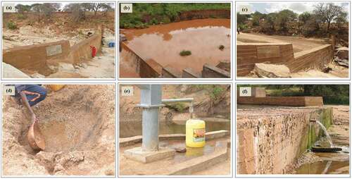
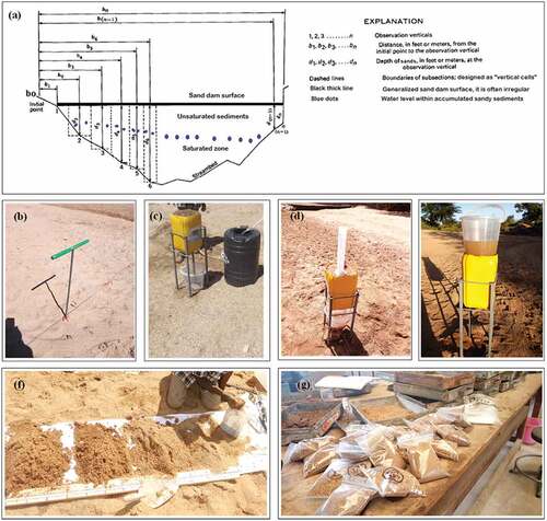
Water supply in drylands is still today’s big challenge that rural dwellers face in water footprints of domestic water supply, agricultural production, and livestock farming (Doreau et al., 2012; Mancosu et al., 2015). Drylands cover 41% of the Earth’s land area and are home to more than 2 billion people, of which 90% live in developing countries (Anton & Shelton, 2011; Prăvălie, 2016). In general, East African drylands occupy about 5,083,000 km² (i.e. 81% of the total surface area) and over half of dwellers live below the poverty line (Flintan et al., 2013; Jama & Zeila, 2005; De Leeuw et al., 2014). Kenya, in particular, drylands occupy nearly 89% of the country’s landmass (GoK, 2012), and support the livelihoods to about 38% of the total population, about 75% of the national livestock, and 90% of the wildlife (Muthini et al., 2014; Njoka et al., 2016). In addition, only 12.8% of the rural population has access to piped water and about 41% still depend on unimproved water sources, such as ponds, shallow wells and rivers (Semanaz, 2018). These statistics indicate a high water demand-supply disparity, translated into chronic water scarcity. The latter is not only limited to the lack of sufficient water resources to meet water demands but also leads to declining water quality. This, in turn, can lead to water-borne diseases and other health problems(Du Plessis, 2019). Many people in rural Kenya experience annually severe food insecurity and water scarcity, exacerbated, from time to time, by climate change. The worst feature of this climate change is the irregularity of the rainfall, resulting in severe droughts which afflict the region by causing the drying-up of water resources, land degradation, and crops destruction (FEWS, 2019). All of these situations mentioned above led local people to find out all possible ways to cope with water scarcity and food insecurity by maximizing the rainfall harvest. After multiple trials, they came up with in-situ rainwater harvesting (RWH) structures. These are built across seasonal riverbeds to retain and store stormwater during the rainy season, with minimal evaporation losses (Mutiso & Thompson, 1987). The first RWH system of this type in Kenya was built in 1958 at Mukongwe on the Muewe River in the former Kitui District, and at that time, it was referred to as a sub-surface dam because it stores water underneath the surface (Muyanga & Mutua, 2000; Thomas, 1999). The actual sand dams began to take shape from 1978 after the completion of the first one by the local NGO, the Utooni Development Organization (UDO) led by the late Joshua Silu Mukusya (1949–2011), a true visionary and one of the original sand dam pioneers (Maddrell & Neal, 2013; Stern & Stern, 2011). In 1985, the UK-based charity NGO (Excellent Development Ltd) sent expeditions to Kenya, Kitui District to support UDO to build more sand dams (Maddrell & Neal, 2013). Since then, this technology gained momentum as it started being supported by local, national, and international non-governmental organizations (NGOs), faith-based organizations (FBOs), and community-based organizations (CBOs). Through initiatives of rural water supply and sanitation, the aforementioned organizations helped local dwellers to construct many dams. They provided the financial funds, technical assistance, and construction material supplies (Ertsen et al., 2005; Maddrell & Neal, 2013; Muyanga & Mutua, 2000). All of these entities contributed to the increasing number and current structure of these RWH systems. After this improvement process, they were referred to as “sand-storage dams” (SSDs) or simply “sand dams” (SDs). These systems are simply reinforced concrete or stone masonry walls built across seasonal sandy rivers (Figure 1 a) in drylands to trap both runoff and sediments during the rainy season (Figure 1 b). Upon drying, mature SDs form shallow aquifers (Figure 1 c) storing water in the pore spaces within sands accumulated behind SD walls (Stern & Stern, 2011). These formed aquifers are then exploited in the dry season for domestic, irrigation, and cattle watering purposes (see Figure 1 d and e). As indicated in Figure 1 c, collected water gets filtered as it infiltrates within sand layers. The thick topmost layer of sand is thought to protect the stored water against evaporation losses and surface contamination (Maddrell, 2016). This layer and subsequent layers are also thought to be able to purify the captured stormwater to the level of making it safer to drink (Hussey, 2007; Maddrell, 2016; Ryan & Elsner, 2016). To access the stored water, people have to dig scoop holes into sediments (see Figure 1 d) or pump it via shallow wells installed deep enough to tap into riverbeds (see Figure 1 e), and/or via riverbed infiltration gallery (see Figure 1 f). Among these methods, shallow wells are often thought to provide more palatable water as the captured stormwater gets filtered as it passes through sand layers. But, all of them provide less potable water as microbial contaminants have been detected in each of them (Abila et al., 2012; Quinn, Parker, et al., 2018; Wandiga, 2015).

Figure 1. Construction and operation principles of sand dams: (a)–(c) field views of sand dam systems before, during and after rainfall events respectively; (d) water abstraction via scoop holes, (e) shallow wells, and (f) riverbed infiltration gallery. Photo credits: A–E, The Water Project, Inc./Kenya, and F: .Maddrell and Neal (2012)

Despite these apparent water quality problems, the number of SDs continues to increase considerably from year to year. Many local, national and international NGOs and FBOs contributed to this increase. They helped local CBOs, locally known as self-help groups (SHGs) to construct more SDs as a result of provided funds, materials and technical assistance (Van der Steen, 2015). Although the current number of SDs constructed so far is not known, about 1,800 are estimated to have been built in Kitui County alone (Van Dalen et al., 2018). Other many more have also been constructed and are still being constructed in other ASAL counties. This has made Kenya renowned for having a large number of SDs and is considered as the home of this technology because more than half of the sand dams and similar systems in the world’s drylands are found in Kenya (Maddrell & Neal, 2013). However, this technology was and is still used in many other countries with similar dry environments such as the U.S.A., Thailand, Zimbabwe, Ethiopia, Namibia, etc. (Hussey, 2007; Neal, 2012) as indicated in the supplemental Figure S1.

Currently, SDs play a big role in the domestic water supply in rural Kenya. By way of example, about 90% of the population in Makueni County use SDs as the main source of domestic water supply (Kalungu et al., 2015). From this perspective, SDs’ capabilities to provide enough water quantity of reasonable quality have become major topics of concern among academic researchers. As a result, numerous empirical and theoretical reproducible studies about SDs were done on various aspects. Specifically, some studies focused on hydrology and hydraulics of SDs (Hoogmoed, 2007; Hut et al., 2008; Quilis et al., 2009; Quinn et al., 2019; Yifru, 2018). Others focused on their cost-effectiveness (De Trincheria et al., 2015a; (Lasage & Verburg, 2015); their water quality (Abila et al., 2012; Avis, ; Kitheka, 2016; Quinn et al., 2018; Wandiga, 2015); their use in agriculture (Leal Filho & De Trincheria, 2018; Villani et al., 2018), their domestic use (Lasage et al., 2015; Maddrell, 2016; Mutiso & Thompson, 1987); their impact on environment (Ryan & Elsner, 2016; Neal, 2012; Aerts et al., 2007; Lasage et al., 2008; Manzi & Kuria, 2011; Lasage & Andela, 2011; Eisma et al., 2021; Eisma et al. (2021) and finally, their socio-economic impact (Lasage et al., 2008; Villani et al., 2018). However, few of these studies have demonstrated how effective SD systems are in fulfilling their intended primary functions, namely stormwater capturing and storing it, improving its quality, protecting it from contamination and evaporation losses, and finally providing sufficient water. For each of these functions, there is an associated performance indicator. All of these indicators form a comprehensive package of measurable metrics that can help gauge the performance levels of SDs and judge their effectiveness. Therefore, we conducted this study to evaluate the effectiveness of sand-dam technologies in fulfilling their primary functions by determining different operational performance indicators (OPIs). Assessed OPIs included stormwater-capture efficiency, water-saving efficiency, volumetric and temporal water supply reliabilities, water loss percentage, impact of evaporation losses and water loss control efficiency, and water quality compliance.

2. Materials and methods

2.1. Study area

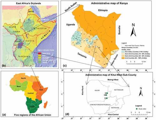
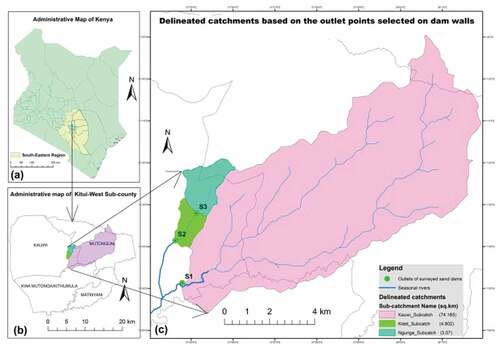
This study was conducted in East Africa (Figure 2 a and b), in a semi-arid region of south-eastern Kenya (Figure 2 c), more precisely in Kitui-West Constituency (Figure 2 d). This constituency covers an area of about 667.2 km2 and the three sites were selected within as indicated with S1, S2 and S3 (see Figure 2 d). These three sites are sand dams located on seasonal sand rivers, namely Kauwi River (1°14ʹ57.82” S and 37°54ʹ47.48” E), Kiteti River (1°13ʹ51.86” S and 37°54ʹ38.00” E) and Ngunga Sya Nthi River (1°13ʹ12.71” S and 37°55ʹ2.80” E). The whole study area and the region in general falls under the semi-arid climate (about 30–84% of aridity) as indicated in (Figure 2 c). This study region lies between the altitudes of 400 m and 1800 m above mean sea level (Njoka et al., 2016), and is characterized by precipitation below the potential evapotranspiration (PET) with two distinct rainy and dry seasons (Gladys, 2017; GoK, 2019; Mutati et al., 2018). The two rainy seasons are “long-rains” season (mid-March to late May), also known as the MAM season, and the “short-rains” season (October to late December), also termed as the OND season. These rainy seasons alternate with two dry seasons, namely the long cool dry season (June–September) and the short hot dry season (late December–mid-March) as shown in Figure 3. The annual precipitation ranges between 250 mm and 1,050 mm with 40% reliability for the long rains season and 66% for the short rains season (Mwamati et al., 2017). The annual potential evaporation rates vary from 1,500 and 1,600 mm and with temperatures ranging from between 14°C and 34°C with mean maxima of 28–34°C and minima of 14–22°C of 28–34°C and minima of 14–22°C all over the year (Kitheka, 2016; Mwamati et al., 2017).

Figure 2. Map showing the study area and locations of study sites (d) in the drylands of Kenya (c), East-Africa (a,b).

According to the living conditions survey in the study area, about 86% of the populations live in rural areas, and 58% of them use unimproved water sources (Kenya Ministry of Health, 2017). Domestic water sources depend on rainfall patterns. The water supply from piped systems covers only 8% and the water consumption rate per person per day varies between 10 and 13 l (GoK, 2019). This rate is below the recommended rate of at least 20 l per person per day by World Health Organization (Reed & Reed, 2013). Local people heavily depend on the harvested rainfall due to lack of modern water production and distribution pipeline systems. The worsening situation is that those rainwater harvesting sources get dry as fast as possible after the rainy season. Therefore, these rural people depend on buying water from private or government-sponsored deep boreholes/kiosks at an average price of 3 Ksh ($0.03) per a 20-litre jerrycan (GoK, 2019). The major RWH systems include earth dams, pans, ponds, sand dams, shallow wells, rock catchments, and rooftop catchments. Among these systems, SDs and their dependent systems, namely (shallow wells (19%), traditional river wells (22%), and rock catchments (2%) constitute roughly 43% of all main water sources in the county (GoK, 2020). Therefore, SD systems play a significant role in the rural water supply in the drylands.

2.2. Data collection and analysis methods

Data used in this paper were collected in three SDs, that were purposively selected from 91 SDs visited during sites reconnaissance. They were selected on the basis of having some water storage, being easily accessible and categorically representative. They were studied from early February to early October (Figure 3), the period during which the MAM rainy season was the target as the major rainwater harvesting period, the JJAS long dry season as the water use period and OND short-rains season as groundwater replenishment period. This kind of investigation setup makes possible the determination of whether the water harvested during the MAM season can used to effectively bridge the long dry season to the next rainy season. To achieve this, different data including SD dimensions, sand volumes, catchment characteristics, water quality parameters, rainfall and temperature records, were collected as detailed in the following sub-sections.

Figure 3. Synopsis of seasonal rainfall and temperature patterns in the study (2018 data of Kitui meteorological station).

2.2.1. Sediment characteristics and analysis methods

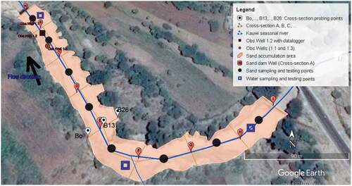
Water volumes that can be harvested by SDs are based on sediment characteristics including sand accumulation coverage areas, volumes of accumulated sands, their porosity and specific yield, and on precipitation patterns. Sediment characteristics collected included three data sets. The first set included depths, sand coverage areas, cross-sectional areas, and volumes of sands. The second set included three types of porosity (total, drainable and residual). The third data set included sediment texture (proportions of sand, silt and clay content) and particle size distribution (PSD) curve parameters (effective particle size, coefficients of uniformly and curvature, and grade category). Each of these data sets were collected from field surveys that consisted of subdividing each of the three investigated SDs into cross-sectional zones (Figure 4).

Figure 4. The plan view of the typical field setup (prepared in Google Earth) at S1 (Kwa Malombe SD, Kauwi River) for measuring sediment properties and water storage capacities.

The first data set was collected by adapting the U.S. Geological Survey mid-section method of streamflow measurement (Rantz, 1982) as indicated in Figure 5 (a) to measure volumes of deposited sands. This method consists of subdividing the three experimental SDs into horizontal transect zones (see Figure 4). On each horizontal transect (A, B, …, Z), sediment depths were estimated with a 2.5 m-long solid steel round rod (Figure 5 b) at one-meter interval horizontal points (see B₀, B₁, B₃, …, B_n in Figure 4.Error! Reference source not found.). Penetration depths of the rod were measured with a tape measure and properly recorded. The recorded depth data points were 413 from 26 transects, including 241 from 9 transects (S1), 105 from 10 transects (S2), and 67 from 7 transects (S3). We used these data to compute sediment volumes (V_SD) and deposition surface areas (A_SD) using the following equations:

(1) $V_{\mathit{SD}}\left(m^3\right)=\sum _{\mathit{i}=1}^n\left(A_i\times L_i\right)\mathit{with}{A}_i=\sum _{\mathit{i}=1}^m{w}_i\times d_i$(1)

(2) $A_{\mathit{SD}}\left(m^2\right)=\sum _{\mathit{i}=1}^n\left[\frac{1}{2}\left(W_i+W_{\mathit{i}+1}\right)\times L_i\right]$(2)

Figure 5. Field setup for measuring main sediment characteristics: (a) measuring procedure of sediment volumes and cross-sectional areas (adapted from Rantz, 1982, P.81); (b) sediment depth probing using the steel rod; (c), (d) and (e) porosity measurement by saturation of sand samples; (g) collection of sand samples, (g) sand samples for sieve analysis in a laboratory.

where n and m are numbers of transects and horizontal interval widths; A_i is the cross-sectional area of the i^th cross-section, L_i is the length between two consecutive cross-sections, w_i and d_i are width and depth of i^th vertical subsection cell; Wi and W_i+1 are the top widths of consecutive cross-sections along with the longitudinal profile.

Sand volumes (V_SD) obtained with Equations (1)(1) $V_{\mathit{SD}}\left(m^3\right)=\sum _{\mathit{i}=1}^n\left(A_i\times L_i\right)\mathit{with}{A}_i=\sum _{\mathit{i}=1}^m{w}_i\times d_i$(1) and (2(2) $A_{\mathit{SD}}\left(m^2\right)=\sum _{\mathit{i}=1}^n\left[\frac{1}{2}\left(W_i+W_{\mathit{i}+1}\right)\times L_i\right]$(2) ) were contrasted with those obtained with the three theoretical estimates of accumulated sands. These theoretical estimation methods included the right triangular pyramid (Equation 3a(3a) $V_{\mathit{SD}}=\left(W_{max}\times D_{max}\times L_{max}\right)/6\times f_{\mathit{sh}}$(3a) ) that significantly distorts the relative size of the bottom width to a line (see the green line in Figure 6 a), the rectangular prism (Equation 3b(3b) $V_{\mathit{SD}}=W_{max}\times D_{max}\times L_{max}\times f_{\mathit{sh}}$(3b) ) that circumscribes accumulated sediments in SD (see the purple line in Figure 6 b), and the trapezoidal prism (Equation 3c(3c) $V_{\mathit{SD}}=\left[1/2\times (W_{max}+W_b)\times D_{max}\right]\times L_{max}\times \mathit{f}{\mathit{\hspace{0.17em}}}_{\mathit{sh}}$(3c) ) that describes the top and bottom bases as flat areas (see dark red lines in Figure 6 b). The hypothetical cross-sections of these solids considered as their bases are shown in Figure 6 (c) via the cutting plane line C-C (see Figure 6 b) and corresponding volumes were calculated as follows:

(3a) $V_{\mathit{SD}}=\left(W_{max}\times D_{max}\times L_{max}\right)/6\times f_{\mathit{sh}}$(3a)

(3b) $V_{\mathit{SD}}=W_{max}\times D_{max}\times L_{max}\times f_{\mathit{sh}}$(3b)

(3c) $V_{\mathit{SD}}=\left[1/2\times (W_{max}+W_b)\times D_{max}\right]\times L_{max}\times \mathit{f}{\mathit{\hspace{0.17em}}}_{\mathit{sh}}$(3c)

Figure 6. Schematic representation of the simplified geometry of SD systems: (a) Longitudinal Section View (Red arrow B), (b) Plan View (Red arrow A), and (c) Possible cross-sectional views via section C-C in the SD wall (Red arrow C).

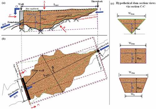
Where V_SD is the volume of sediments (m³), D_max is the max. sediment depth (m), W_max is the max. top width (m), W_b is the max. bottom width (m), L_max is the max. throwback length (m), and f_sh is the shape adjustment factor.

The second data set was about the porosity of deposited sediments in the three experimental SDs. Three porosity variables were measured in the field by the sand sample saturation method (Anovitz & Cole, 2015; Matko, 2003; MoWI, 2015b). This method consists in comparing volumes of water absorbed in dry sands (see Figure 5 c) and drained out the water in the bucket (see Figure 5 d & e) to their respective initial volumes (volume of the container, V_c). The volumes of water that were poured into the dry sand (V_w), water drained out (V_d) and water retained (V_r) were recorded. Porosity results were obtained from the following equations:

(4a) ${\phi }_T=V_w/V_c\times 100$(4a)

(4b) ${\phi }_d=V_d/V_c\times 100$(4b)

(4c) ${\phi }_r=\left(V_w-V_d\right)/V_c$(4c)

where ϕ_T is the total porosity (%), ϕ_d is the drainable porosity (%), and ϕ_r is the residual porosity (%). The ϕ_d is also known as “specific yield” and is equal to (ϕ_T -ϕ_r).

The third data set was derived from sieve analysis tests to assess the particle size distribution (PSD) of accumulated sediments by using the British Standard Sieving Test Procedure. The BS (882:1992) sieve series whose nominal openings (10.00, 5.00, 2.36, 1.18, 0.60, 0.30, and 0.15) were used (BSI, 2002). Sediment samples were collected (see Figure 5 f) for grain size analysis (see Figure 5 g) from the same points as field porosity-measuring points (see the black target points in Figure 4). Sand samples were labeled as “S1AB19” to mean that the sample was taken from site S1 in the intersectional zone AB at 19 m from the SD wall. Sieve analysis results were used to determine the particle size distribution (PSD) curve characteristics (d₁₀, d₃₀, and d₆₀), measures of gradation, namely uniformity coefficient (Cu) and coefficient of curvature (Cc), and content percentages of particle size ranges (fines, sands, and gravels) using the formulas reported in the soil mechanics laboratory manual (Das, 2002). With Cu and Cc values, sediments were classified as well-graded (WG) if Cu ≥ 6 and 1< Cc < 3, poorly graded (PG) for Cu < 6 and 1< Cc < 3, and gap-graded (GG) if 1> Cc > 3.

2.2.2. Estimation of Water storage capacities

With volumes of sediments estimated with Equations (1)(1) $V_{\mathit{SD}}\left(m^3\right)=\sum _{\mathit{i}=1}^n\left(A_i\times L_i\right)\mathit{with}{A}_i=\sum _{\mathit{i}=1}^m{w}_i\times d_i$(1) and (3), the volumes of maximum storable (V_MW), extractable (V_EW), and residual (V_RW) water were determined as follows:

(5a) $V_{\mathit{MW}}=V_{\mathit{SD}}\times {\phi }_T(\mathrm{\%})$(5a)

(5b) $V_{\mathit{EW}}=V_{\mathit{SD}}\times {\phi }_d(\mathrm{\%})$(5b)

(5c) $V_{\mathit{RW}}=V_{\mathit{SD}}\times {\phi }_r(\mathrm{\%})$(5c)

In order to relate water storage capacity with maximum water depth, the water harvested in each month of the study period was estimated using initial and maximum monthly water levels. By applying the right-angled triangle geometry of riverbeds (see the dashed green line in Figure 6 a), the throwback length (L_max) was expressed in terms of fluctuating water levels (h) and bed slope (S_o) as L_max = h × 100/S_o with 0 ≤ h ≤ D_max (MoWI, 2015b). By incorporating this relationship into Equation (2b)(2) $A_{\mathit{SD}}\left(m^2\right)=\sum _{\mathit{i}=1}^n\left[\frac{1}{2}\left(W_i+W_{\mathit{i}+1}\right)\times L_i\right]$(2) and obtained expressions into Equations (5), the latter become expressed as follows:

(6a) $V_{\mathit{MW}}=W_{max}\times \left(h^2\times 100/S_o\right)\times {\phi }_T\times f_{\mathit{sh}}$(6a)

(6b) $V_{\mathit{EW}}=W_{max}\times \left(h^2\times 100/S_o\right)\times {\phi }_d\times f_{\mathit{sh}}$(6b)

(6c) $V_{\mathit{RW}}=W_{max}\times \left(h^2\times 100/S_o\right)\times {\phi }_r\times f_{\mathit{sh}}$(6c)

Where h is the fluctuating water level (m); W_max, ϕ_T, ϕ_d, ϕ_r and f_sh are as previously defined in Equations (3)

2.2.3. Measurement and analysis of water levels

To obtain daily water-level data as input variables in Equations (6), non-vented water-level loggers (HOBO U20L-04, Onset Computer Corporation, Inc., Bourne, MA, USA) were used. Technical specifications and deployment procedures of these data loggers are provided in the HOBO-U20L user manual (Onset Computer Corporation, 2018). To perform this task, these data loggers were deployed into three temporary observation wells (TOWs) located at 39.5 m, 17.5, and 11.5 m from dam walls of investigated SDs (S1, S2, and S3) respectively. The structure of TOWs is schematically illustrated in Figure 7 and their field views are shown in Figure 8.

Figure 7. The field measurement set-up for water levels level in temporary monitoring wells (See annotations in Table 1).

Figure 8. Field setup for water level monitoring in the SD (S1), Kauwi river: (a) Temporary observation well (TOW), (b) Field view of data loggers used, (c, d, e) the TOW wellhead after rainfall events and during the dry season.

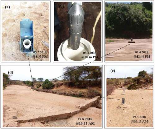
Table 1. Field deployment details of Data loggers in temporary observation wells in the investigated sites

Data logger Deployment details	Site 1	Site 2	Site 3
Position of the observation well with the data logger from the dam wall	390	175	115
Well diameter (2 R), Radius (R)	10	7.6	10
Well casing length (EL) above Ground Level (GL)	50	50	45
Depth to water (DW) with reference to well cap and groundwater level (GW)	138.3	112.5	139.9
Data logger deployment depth (DL)	153	125	145
Well depth (WD)	165	145	155
Sediment depth (SD)	130	110	120
Total depth (TD) from bedrock up to the well cap	180	160	165
Initial water column above the data logger (WCd)	14.7	12.5	5.1
Initial water column in the well (WCw) or the pressure head (ψ)	26.7	32.5	15.1
Free space below the data logger sensor tip (BD)	12	20	10
Elevation head, Z	15	15	10
Initial hydraulic head, h (=WCd+BD+Z)	41.7	47.5	25.1
All measurements are in cm.

After the installation of TOWs (Figure 8 a), data loggers were deployed inside (Figure 8 b) to record the 10-min interval water level fluctuations. These data loggers were then left enclosed inside the lockable well caps (Figure 8 c, e) to protect them from damages, theft, and or being washed away during heavy rains. Deployment and positioning details of data loggers in the TOWs with reference to the top of the well casing (TOC), are shown in Table 1. TOWs with data loggers were periodically visited to read out data loggers to generate data files via the procedure described in Figure 9 (a).

Figure 9. Water level data analysis processes: (a) Pre-processing procedures (a₁: Observation well, a₂: HOBO U20L water level logger, a₃: Base-U-4 Optic USB Base Station for configuration and data offload, a₄: a general-purpose laptop), and (b) Post-processing procedures (b₁: data view in HOBOware Software, b₂: data view in M/S Excel).

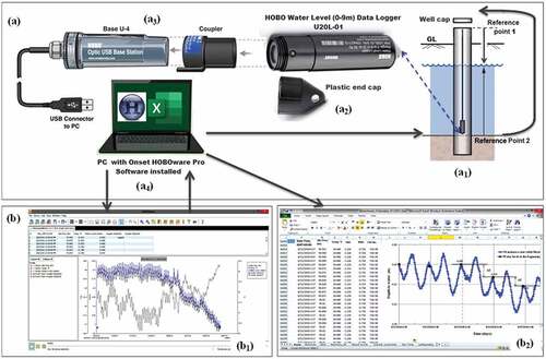
These offloaded (filename.hobo) files were post-processed using the HOBOware’s Barometric Compensation Assistant (BCA) to convert the recorded water pressure data series (kPa) into water level data series (m), and were saved as filename.hproj files (see Figure 9 b₁). The BCA Tool was also used to display, edit, plot, and export data tables (filename.csv files) and graphs. Details of how water depths are obtained from pressure readings are provided in the BCA Technical Guide (Onset Computer Corporation, 2008). The post-processed data files were then manipulated in Excel (see Figure 9 b₂) to generate descriptive statistics of water levels (Min., Max., Mean ± SD) and water-level changes (±Δz) between consecutive days.

2.2.4. Rainfall and temperature data

Daily Rainfall data used in this study were sourced from Kenya Water Resources Management Authority (WARMA) for the Kitui meteorological station. Two temperature datasets were collected for estimating evaporation losses. Borehole water temperature data were collected with the same devices (Hobo Data loggers) as water levels and were used to estimate ground water evaporation. Air temperature data were sourced from the World Weather Online (2019) for Kitui during the period of study. Together with parameters of delineated catchments, rainfall data were used to estimate runoff, rainfall volumes, and evapotranspiration (ET).

2.2.5. Water balance analysis

The water balance analysis consisted of estimating the amount of water that can be captured, abstracted and lost from the experimental SDs. The latter captures a partial portion of the catchment runoff estimated from water budget components illustrated in

Figure 10 (a). At the catchment scale, the equation governing the water balance is as follows:

Figure 10. Schematic representation of major water balance components: (a) at the catchment scale and (b) at the site scale.

(7) $Q_R=\mathit{P}-(\mathit{ET}+\mathit{F}+\mathrm{\Delta S})$(7)

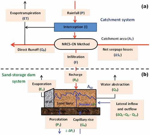
where Q_R, P, ET, F and ΔS are surface runoff, precipitation, evapotranspiration, infiltration and change in storage, respectively

At the site scale, water balance components (WBCs) in SDs are governed by the amount of the recharge as indicated in

Figure 10 (b). The sand-dam water balance equation is expressed as:

(8) $R_E=Q_A+E_V+P_L+\mathrm{\Delta }{S}_D$(8)

Where R_E is the recharge, Q_A is water abstraction (domestic use, irrigation and animals), E_V is evaporation, P_L is the percolation or seepage losses and ΔS is the change in storage within SD sediments.

2.2.5.1. Estimation of direct surface runoff volumes

Volumes of incoming runoff for three selected SDs were estimated using rainfall records of the study area and major catchment characteristics (areas, curve numbers, slopes and stream lengths). Potential runoff-contributing catchment areas (PRCAs) for three SDs were delineated with the Watershed Modeling System Software (WMS v10.1; Aquaveo LLC: Provo, Utah, United States). This software uses online data sources to automatically generate the digital elevation model (DEM) data for the selected areas. Only two external inputs in this automatic delineation process were outlet coordinates taken by a hand-held GPS, and global land use-land cover (LULC) data: A table relating land use IDs and soil cover characteristics to curve numbers for each hydrologic soil group (see the supplemental Table S1). Detailed procedures of this automated watershed delineation are deeply described in the WMS user manual (Aquaveo, 2016). Two major WMS output files were shapefiles (filename.shp) for maps and table text files (report.txt) for watershed data (CN values, catchment areas and land use descriptions). Obtained CN values were contrasted with those describing arid and semiarid climates (see the supplemental Table S2). Shapefiles were later imported into ArcGIS (v10.0) to produce the final catchment maps. With obtained catchment areas (Ac) and CN values, runoff (Q_R) and rainfall (Q_P) volumes for the three SD sites were estimated with the NRCS Runoff Curve Number method (NRCS, 1986):

(9a) $Q_R(\mathit{mm})=\left\{\begin{array}{c}\frac{{\left(\mathit{P}-\mathit{Ia}\right)}^2}{\mathit{P}-\mathit{Ia}+\mathit{S}}\mathit{for}\mathit{P}\ge \mathit{Ia};\mathit{with}\mathit{Ia}=0.2\mathit{S}\\ 0\mathit{for}\mathit{P}<\mathit{Ia}\end{array}\right.$(9a)

(9b) $Q_R(\mathit{mm})=\frac{{\left(P_e\right)}^2}{p_e+\mathit{S}}\mathit{with}{P}_e=\mathit{P}-\mathit{Ia},\mathit{and}\mathit{S}=\frac{25400}{\mathit{CN}}-254$(9b)

(9c) $Q_R(m^3)=Q_R(\mathit{mm})\times f_{\mathit{c}}(10m^3/\mathit{ha})\times A_c(\mathit{ha})$(9c)

(10) $Q_P(m^3)=P_e(\mathit{mm})\times f_{\mathit{c}}(10m^3/\mathit{ha})\times A_c(\mathit{ha})$(10)

Where P_e is the effective precipitation (mm); Ia is initial abstraction (mm) which is all losses before runoff begins, S is the potential maximum watershed retention after runoff begins (mm); CN is the curve number ranging from 0 (no runoff potential, perfectly permeable soil) to 100 (high runoff potential, perfectly impermeable soil), f_c is the unit conversion factor (1 mm = 10 m³/ha).

2.2.5.2. Estimation of daily water abstraction

Volumes of water abstracted from the SDs per day (Q_A) were estimated with the equations derived from analytical procedures detailed in Table 2.

Table 2. Detailed procedure followed to determine the volume of water abstracted from sand dams per day

Water demand Components	Steps	Estimation procedures
Livestock water demand (LWD)	(1)	One Livestock Unit (LU) is assumed to consume 50 l/head/day of water ((MoWI, 2015b). The number of LUs is estimated per hectare based on the annual rainfall pattern of the region under consideration (See the supplemental Error! Reference source not found., Col.1)
	(2)	Once the annual rainfall (mm) is known, the number of LUs per hectare is then estimated. In the study area, the annual rainfall ranges from 500 to 1050 mm (Gladys, 2017; Mutunga et al., 2018; Mutati et al., 2018). Therefore, after range interpolation, the number of LUs per corresponding to this rainfall range rainfall was found to be 0.92 LU/ha.
	(3)	As the catchment areas corresponding to three studied sand-storage dams (SDs) were determined, the number of Livestock units per delineated catchment area (Ac) was obtained from the following expression: $\mathit{LUs}{}_{\mathit{per}\mathit{catchment}}=0.92\frac{\mathit{LUs}}{\mathit{ha}}\times A_c(\mathit{ha})(11\mathit{a})$
	(4)	The obtained numbers of livestock units from Equation (11a)$\mathit{LUs}{}_{\mathit{per}\mathit{catchment}}=0.92\frac{\mathit{LUs}}{\mathit{ha}}\times A_c(\mathit{ha})(11\mathit{a})$ cannot be attributed to one SD as normally SDs are constricted in cascades along seasonal rivers (see the supplemental Figure S2 (c)). Therefore, we made an assumption that the number should be distributed per reach of rivers within each delineated catchment area. Based on field observations, the spacing of SDs in cascade along seasonal river channels may vary from 100 m to 5 km depending on the nature of seasonal river meanders. In this study, we assumed the spacing of 1 km between consecutive SDs along river networks within delineated catchments. River network lengths in each delineated catchment were easily estimated by the measure tool of the (WMS v10.1) software. Measured lengths were obtained as 30,452.90 m in site S1 resulting in 30 reaches; 5,652.45 m in site S2 resulting in 6 reaches and 3,165.27 m in site S3 resulting in 3 reaches using the following Equation: $\mathit{No}.\mathit{of}\mathit{reaches}(N_R)=\frac{\mathit{River}\mathit{Network}\mathit{Length}}{\mathit{Assumed}\mathit{SSD}\mathit{spacing}}(11\mathit{b})$
	(5)	The number of livestock units (LU) per reach (LUR) in each SD considered as number of livestock units per SD (NLU) and was obtained as the ratio of results of Equations (11a)$\mathit{LUs}{}_{\mathit{per}\mathit{catchment}}=0.92\frac{\mathit{LUs}}{\mathit{ha}}\times A_c(\mathit{ha})(11\mathit{a})$ and (11b$\mathit{No}.\mathit{of}\mathit{reaches}(N_R)=\frac{\mathit{River}\mathit{Network}\mathit{Length}}{\mathit{Assumed}\mathit{SSD}\mathit{spacing}}(11\mathit{b})$) as follows: $\mathit{L}{U}_R=\frac{\mathit{LUs}\mathit{per}\mathit{catchment}}{\mathit{No}.\mathit{of}\mathit{reaches}}=\frac{A_c(\mathit{ha})\times \mathit{LU}(\mathit{no}./\mathit{ha})}{N_R(\mathit{no}.)}(11\mathit{c})$
Domestic Water Demand (DWD)	(6)	The minimum basic water access is set to be 20 litres per capita per day (Lpcd) was assumed in estimation of domestic water demand (WHO/UNICEF, 2000; WHO, 2003).
	(7)	Numbers of people (NP) per SD were extracted from the inventory of water projects in Kitui-West Sub-County, provided by the water supply and sanitation office. The domestic water demand (QD) was calculated as follows: $Q_{\mathit{PD}}=N_P\times L_{\mathit{pcd}}(11\mathit{d})$
Irrigation Water Demand (IWD)	(8)	It is also assumed that some water may be abstracted for irrigation purpose; the scheme irrigation water demand(QSID) was estimated with the irrigation command area (NICA) and the daily irrigation water requirement (Ldiw), expressed in l/day/ha or mm/day (see the supplemental Error! Reference source not found.) as follows: $Q_{\mathit{SID}}=A_{\mathit{IC}}(\mathit{ha})\times L_{\mathit{diw}}(\mathit{mm}/\mathit{day})\times f_c,\mathit{with}{f}_c\mathit{as}1\mathit{mm}=10m^3/\mathit{ha}(11\mathit{e})$
Combination (LWD, DWD and IWD)	(9)	Estimated LUR values (step 5) and information described in steps 6, 7 and 8 were used to estimate daily water abstraction (QA) for each SD as follows: $Q_A=\left[\left(N_{\mathit{LU}}\times L_{\mathit{hd}}\right)+\left(N_p\times L_{\mathit{pd}}\right)+\left(A_{\mathit{IC}}\times L_{\mathit{diw}}\right)\right]\times f_c(11\mathit{f})$ If there is no irrigation practices in the surroundings of SD systems, Equation (11f)$Q_A=\left[\left(N_{\mathit{LU}}\times L_{\mathit{hd}}\right)+\left(N_p\times L_{\mathit{pd}}\right)+\left(A_{\mathit{IC}}\times L_{\mathit{diw}}\right)\right]\times f_c(11\mathit{f})$ become as follows: $Q_A=\left[\left(N_{\mathit{LU}}\times L_{\mathit{hd}}\right)+\left(N_p\times L_{\mathit{pd}}\right)\right]\times f_c(11\mathit{g})$ Where: Np. is the number of people assigned to each sand-storage dam (SD) NLU is the number of livestock units per sand dam Lpd is the per capita daily consumption rate (Liters/person/day) fc is the unit conversion factor (equal to 0.001 from liters to cubic meters)

Source: Authors ‘elaboration on based on the sources cited herein

To compare daily abstraction volumes obtained from Equations (11f and 11g) in Table 2 with other water-balance variables expressed in mm/day, (Q_A) values (m³/day) were converted into equivalent depths of removed water (mm/day) by using the following equation (Fitts, 2002):

(12) $h_A=Q_A/S_y\times A_{\mathit{SD}}$(12)

where h_A is the equivalent depth of water-level decline within sand sediments (m/day), S_y is the specific yield (%), and A_SD is the sand surface area (m²)

2.2.5.3. Estimation of water losses in SD systems

Seepage and evaporation losses were estimated from the water table exchange flux. This exchange flux describes both rates of water gain and loss in the sand dam aquifer. Water gains and losses are indicated by the rise and fall of water levels around the interface between saturated and unsaturated zones. This water gain and loss exchange flux (E_GL) was estimated as follows (Balugani et al., 2016):

(13) $E_{\mathit{GL}}(\mathit{mm}/\mathit{day})=\left({\theta }_{\mathit{sat}}-{\theta }_r\right)\times \mathit{d}{Z}_{\mathit{WT}}/\mathit{dt}$(13)

where E_GL is the water gain-loss fluctuation flux in the function of water depth (Z_WT): +ve E_GL values mean recharge or gain and—ve E_GLvalues mean discharge including losses; θ_sat is the water content at saturation (cm³/cm³) considered as the total porosity (ϕ_T), θ_r is the residual water content (cm³/cm³), the term (θ_sat-θ_r) is the specific yield (Sy), ΔZ_WT (> 0, < 0, = 0) is the daily water-level change (see Figure 9 b₂), and t is the time (days).

2.2.5.4. Estimation of Evaporation and seepage losses

Evaporation and percolation losses were estimated from negative E_GL values. Evaporation losses were estimated from recorded temperature data using the empirical Hargreaves-Samani equation (Kra, 2014). Both evaporation and seepage losses were estimated as follows:

(14) $\mathit{E}{T}_p=0.0023\left(T_{\mathit{mean}}+17.8\right){\left({\mathit{T}}_{max}-T_{min}\right)}^{0.5}\mathit{Ra}$(14)

(15) $P_L=E_{\mathit{GL}}(-\mathit{ve})-\mathit{E}{T}_p-h_A$(15)

where T_mean is mean daily temperature (°C), T_max is the maximum daily temperature (°C), T_min is the minimum daily temperature (°C) and Ra is extraterrestrial radiation (MJm⁻²day⁻¹) whose values are readable from Table 2: Daily extraterrestrial radiation (Ra) for different latitudes in Annex 2 of meteorological tables in FAO Irrigation and drainage paper 56 (Allen et al., 1998). Ra values are then converted into mm/day by dividing them with the latent heat of vaporization (λ = 2.45 MJ kg⁻¹).

2.3. Collection and analysis of water samples

2.3.1. Collection of water samples

Water samples were collected at three points in each of the three SD sites as indicated by the blue placemarks in Figure 4. These samples were aseptically collected in triplicates of 500-ml polyethylene bottles from the holes scooped into riverbeds and shallow hand-pump wells. A total of 36 samples were gathered in proportions of 41.7% (S1, n = 15), 38.9% (S2, n = 14) and 19.4% (S3, n = 7) respectively. They were transported to the laboratory in ice boxes for storage and analysis. Five of eighteen tested parameters, namely temperature, pH, turbidity, total dissolved solids (TDS), electrical conductivity (EC), and dissolved oxygen (DO), were measured at the field. The remaining parameters, namely total hardness, sodium, phosphates, nitrates, sulfates, chromium, zinc, copper, manganese, iron, biochemical oxygen demand, Escherichia coli (E.coli), and total coliforms were analyzed in the laboratory. Analyses were performed following the standard operating methods and quality assurance procedures for physicochemical and microbial water quality tests (Hach, 2012). Detailed analytical methods for the tested parameters are provided in the supplemental Table S5.

2.3.2. Analysis of water quality data

Measured concentration values of tested water quality parameters (WQPs) were processed using Excel software to summarize descriptive statistics (min., max., mean, and standard deviation). To achieve this, all concentrations reported as “not detected, ND”, were assigned with zero values as recommended in previous studies (Evans et al., 2020; McGrath et al., 2018). The measured concentrations were also compared to the corresponding maximum allowable concentration limits set in the Kenya Bureau of Standards for natural potable water (KEBS, 2015) and World Health Organization (WHO)’s guidelines for drinking water (WHO, 2017). This helped to determine non-compliance rates of physicochemical and microbiological water quality parameters. These non-compliance rates were calculated as ratios of the number of non-compliant samples for a particular parameter to the total number of analyzed samples (Onyango et al., 2018). Unfortunately, the non-compliance rate does not suffice to disambiguate the impact of one non-compliant parameter on the overall water quality. One parameter may make the whole water objectionable. For instance, the highly turbid or saline water is objectionable to color or salt taste while it may be microbiologically or chemically safe. Therefore, to account for the impact of one detrimental parameter, the water pollution index (WPI) was calculated. This index summarizes and communicates the complex water quality data in a simple, interpretable, and understandable way (Effendi et al., 2015; Suwandana et al., 2011). This index considers the maximum contaminant violation levels and is computed with the equation below, and interpreted as shown in Table 3.

(16) $\mathit{WPI}=\frac{1}{m}\sum _{\mathit{i}=1}^m\sqrt{\frac{{\left(Max\left(C_i/S_i\right)\right)}^2+{\left(1/n{\sum }_{i=1}^n\left(C_i/S_i\right)\right)}^2}{2}}$(16)

Table 3. Water quality classification and its interpretation based on WPI values

Class	WPI Values	Water quality status	Objectionable level	Comments
I	≤ 1	Clean^1	None	Perfectly clean water and disinfection only
II	1–2.5	Fairly clean	Very low	Somewhat clean water and disinfection only
III	2.5–5	Slightly polluted	Low	Minor purification and disinfection
IV	5–10	Moderately polluted	Medium	Moderate purification and disinfection
V	10–15	Polluted	High	Special treatments such as BSFs, CWFs, SODIS, etc.^2
VI	15–20	Very polluted	Very high	Major water treatment processes should be applied
VII	>20	Extremely polluted	Unacceptable	Unsuitable for any use. It may require high-tech treatment methods

¹Water quality is physicochemically fit for drinking purposes as it meets the water quality standards

²BSFs: Biological sand filters; CWFs: Ceramic Water Filters; SODIS: Solar water Disinfection

Source: Compiled from Suwandana et al. (Suwandana et al., 2011) and Effendi & Wardiatno (Effendi et al., 2015)

Where m is the total number of water samples, C_i is the measured concentration value of parameter i, S_i is the standard permissible concentration of parameter i, n is the total number of tested parameters.

2.4. Determination of performance indicators

The selected operational performance indicators (OPIs) include five water quantity-based indicators and two water quality-based indicators (see Table 4). These OPIs helped gauge the effectiveness of SDs in fulfilling their intended functions of capturing stormwater, storing it, improving its quality and protecting it from losses and contamination. All of these OPIs used in this study are defined as they were defined in the cited sources. All of them were expressed in percentage except the WPI presented as numerical aggregation of ratios of actual and permissible concentration values of considered water quality parameters as indicated in Table 3. Performance indicators always require evaluation criteria (Moriasi et al., 2015). For this study, evaluation criteria are described in the last column of Table 5, complemented with those reported in the supplemental Table S6.

Table 4. Summary of computed operational metrics to evaluate the performance of SDs

Criteria	Performance Indicators	Abbrev.(units)	Computational Formula	Adapted /Adopted from	Evaluation criteria^4
Quantity	Catchment runoff efficiency^1	CRE (%)	$\mathrm{CRE}=\frac{\mathrm{Volume}\mathrm{of}\mathrm{estimated}\mathrm{runoff}({\mathrm{V}}_{\mathrm{runoff}})}{\mathrm{Volume}\mathrm{of}\mathrm{rain}({\mathrm{V}}_{\mathrm{rain}})}$	(McCabe & Wolock, 2016)	Good efficiency values should be ≥70%
	Stormwater capture efficiency^2	SCE (%)	$\mathrm{SCE}=\frac{\mathrm{Seasonal}\mathrm{rainwater}\mathrm{storage}(\mathrm{SRS})}{\mathrm{Mean}\mathrm{seasonal}\mathrm{runoff}(\mathrm{MSR})}$	(Lasage & Andela, 2011)
	Water-storage efficiency	WSE (%)	$\mathrm{RSE}=\frac{\mathrm{Seasonal}\mathrm{water}\mathrm{storage}\mathrm{yield}(\mathrm{SWY})}{\mathrm{Total}\mathrm{seasonal}\mathrm{water}\mathrm{storage}(\mathrm{TWS})}$	(Butler & Memon, 2006)
	Runoff event capture ratio	REC (%)	$\mathrm{RSE}=\frac{\mathrm{Seasonal}\mathrm{water}\mathrm{storage}\mathrm{yield}(\mathrm{SWY})}{\mathrm{Total}\mathrm{seasonal}\mathrm{water}\mathrm{storage}(\mathrm{TWS})}$	(Guo & Urbonas, 1996)
	Volume-based reliability^3	RV (%)	${\mathrm{R}}_{\mathrm{V}}=\frac{\mathrm{Seasonal}\mathrm{water}\mathrm{storage}\mathrm{yield}(\mathrm{SWY})}{\mathrm{Total}\mathrm{seasonal}\mathrm{water}\mathrm{demand}(\mathrm{TWD})}$	(Soundharajan et al., 2016)	Good reliability values should be ≥ 70%
	Time-based reliability	RT (%)	${\mathrm{R}}_{\mathrm{T}}=\frac{\mathrm{No}.\mathrm{of}\mathrm{days}\mathrm{the}\mathrm{demand}\mathrm{can}\mathrm{be}\mathrm{met}(\mathrm{NS})}{\mathrm{No}.\mathrm{of}\mathrm{days}\mathrm{in}\mathrm{the}\mathrm{considered}\mathrm{period}(\mathrm{N})}$	(Hanson & Vogel, 2014)
	Evaporative losses index	ELI (%)	$\mathrm{ELI}=\frac{\mathrm{Total}\mathrm{evaporation}\mathrm{losses}(\mathrm{TEL})}{\mathrm{Total}\mathrm{water}\mathrm{losses}(\mathrm{TWL})}$	(Zhao & Gao, 2019)	< 10% little concern, 10–25% Modest concern, 25–35% Interm. concern, 35–50% Signif.concern >50% Critical concern,
	Seepage losses impact	SLI (%)	$\mathrm{SLI}=\frac{\mathrm{Total}\mathrm{seepage}\mathrm{losses}(\mathrm{TSL})}{\mathrm{Total}\mathrm{water}\mathrm{losses}(\mathrm{TWL})}$	(MoWI, 2015b)
	Percentage Water losses index	PLI (%)	$\mathrm{PLI}=\frac{\mathrm{Total}\mathrm{water}\mathrm{losses}(\mathrm{TWL})}{\mathrm{Total}\mathrm{water}\mathrm{storage}(\mathrm{TWS})}$	(Ociepa et al., 2019)
Quality	Microbiological pollution level	MPL (%)	$\mathrm{PLI}=\frac{\mathrm{Number}\mathrm{of}\mathrm{non}-\mathrm{compliant}\mathrm{samples}}{\mathrm{Total}\mathrm{number}\mathrm{of}\mathrm{samples}}$	(Onyango et al., 2018)	Good MPL values ≤ 10%
	Physicochemical pollution index	WPI (-)	See Equation 16(16) $\mathit{WPI}=\frac{1}{m}\sum _{\mathit{i}=1}^m\sqrt{\frac{{\left(Max\left(C_i/S_i\right)\right)}^2+{\left(1/n{\sum }_{i=1}^n\left(C_i/S_i\right)\right)}^2}{2}}$(16)	(Suwandana et al., 2011)	Good WPI values ≤ 1

¹This is the efficiency of the catchment surface in collecting runoff, also known as runoff coefficient.

²This is the property of sand dams, which is the function of sediment volumes and porosity, and the received runoff

³This is also known as the water demand satisfaction rate (WDSR), an indicator of the potential ability of each SD to satisfy the main water demands.

⁴The evaluation criteria for performance indicators established based on literature values compiled in the supplemental Table S6

Table 5. Descriptive rating scales used to gauge the performance of SDs based on calculated PIVs in Table 4

Water quantity-based performance indicators				Water quality-based performance indicators
PIV^1 Range (%)	Reliability^3	Efficiency	Yield/Loss/Impact	Water pollution levels^2	Probable Risk levels^2	Levels of water quality^2
90–100	Extremely reliable	Excellent	Extremely high	Extremely Polluted	Extremely high	Extremely poor
80–90	Highly reliable	Very good	Very high	Very polluted	Very high	Very poor
60–80	Reliable	Good	High	Polluted	High	Poor
40–60	Moderately reliable	Fair	Moderate	Moderately Polluted	Moderate	Fair
20–40	Slightly reliable	Poor	Low	Slightly polluted	Low	Good
10–20	unreliable	Very Poor	Very low	Slightly clean	Very low	Very Good
0–10	Absolutely unreliable	Almost none	Almost none	Clean water	Almost none	Excellent

¹PIV = Performance Indicator’s Value

²Levels of water quality in this context should be understood as levels of non-compliance with considered water quality standards

Source: These threshold range values were summarized from Table 6 to Table 10 in the work of Aboelnga et al. (2019)

Table 6. Synoptic summary of the physical characteristics of the three studied sand dams

Site characteristics	Units	S1	S2	S3	Overall mean (±SD)
Location coordinates
Latitude	DMS	1°14ʹ57.57”S	1°13ʹ51.97”S	1°13ʹ12.77”S	—
Longitude	DMS	37°54ʹ46.96”E	37°54ʹ38.02”E	37°55ʹ2.72”E	—
Physical dimensions
Wall length (m)	m	24.00	11.00	12.00	—
Maximum Wall depth	m	1.75	1.80	1.40	—
Maximum Throwback length (Lmax)	m	354.00	132.00	124	—
Bedslope	m/m	0.0056	0.0056	0.0081
Physical properties of deposited sands
Mean sediment depth (Dmean)	m	0.744	0.455	0.309	0.59(±0.50)
Maximum sediment depth (Dmax)	m	2.1	1.7	0.7	1.52(±0.69)
Sand accumulation plan area (Max.)	m^2	9,336.00	1,274.00	1,024.00	—
Volume (Max.)	m^3	6,964.95	611.78	346.40	—
Mean total porosity	%	34.40	28.06	35.75	32.27(±5.00)
Mean specific yield	%	24.56	19.89	25.92	23.09(±5.12)
Mean percentage content of fines	%	1.26	2.74	1.43	1.89 (±1.71)
Mean percentage content of sands	%	87.18	83.24	85.03	85.08 (±8.86)
Mean percentage content of gravels	%	11.56	14.04	13.54	13.05 (±8.33)
Mean effective particle size (D10)	(mm)	0.30	0.26	0.26	0.27(±0.07)
Mean diameter corresponding to 30% finer (D30)	(mm)	0.57	0.50	0.54	0.53 (±0.19)
Mean diameter corresponding to 60% finer (D60)	(mm)	1.40	1.56	1.27	1.43 (±0.77)
Mean uniformity coefficient (Cu)	—	4.68	6.17	4.79	5.29 (±2.24)
Mean coefficient of curvature (Cc)	—	0.81	0.74	0.94	0.82(±0.28)
Maximum water storage capacity	m^3	2,395.94	171.30	123.84^c	—
Maximum extractable water	m^3	1,710.59	121.68	89.79	—

DMS=Degrees, minutes, seconds; StDev= Standard deviation

Table 7. Computed hydrologic characteristics of catchments corresponding to three experimental SDs

Site ID	Catchment ID	HSG	Land Cover Description	CN (-)	Area (km^2)	Product (CN x A)	Weighted CN (TP/TA)	Watershed Length	Watershed slope (%)	Lag time (hrs)
S1	1B	C	Closed to open (>15) herbaceous vegetation	86	68.658	5904.624
		C	Closed to open (>15) (broadleaved or needlele	70	1.491	104.368
		C	Mosaic vegetation (grassland/shrubland/forest)	73	4.015	293.116
			Total		74.164	6302.108	85	21.293	7.273	2.99
S2	2B	C	Closed to open (>15) herbaceous vegetation	86	3.067	263.762
		C	Closed to open (>15) herbaceous vegetation (g 86)	86	1.603	137.858
		C	Artificial surfaces and associated areas (Urba 91)	91	0.134	12.194
			Total		4.804	413.814	86	3.165	3.412	0.92
S3	3B	C	Closed to open (>15) herbaceous vegetation	86	3.067	263.775	86	2.487	4.374	0.66

Note: HSG = Hydrologic Soil Group, CN = Curve Number, TP = Total Product, TA = Total Area; 1B, 2B and 3B are catchment identifiers in the WMS Model.

Table 8. Summary of major water balance components for three evaluated SDs over the study period

Water balance components				Surveyed sand dams
Water balance components	Abbrev.	Units	Eqn.	Kwa Malombe SD	Kiteti SD	Motomoto SD
				S1	S2	S3
Mean seasonal runoff	MSR	m^3	Eq.9c(9c) $Q_R(m^3)=Q_R(\mathit{mm})\times f_{\mathit{c}}(10m^3/\mathit{ha})\times A_c(\mathit{ha})$(9c)	393,590.59	25,976.75	17,034.42
Mean seasonal precipitation	MSP	m^3	Eq.10(10) $Q_P(m^3)=P_e(\mathit{mm})\times f_{\mathit{c}}(10m^3/\mathit{ha})\times A_c(\mathit{ha})$(10)	675,363.30	44,649.17	28,439.89
Total seasonal water storage	TWS	m^3	Eq.6a(6a) $V_{\mathit{MW}}=W_{max}\times \left(h^2\times 100/S_o\right)\times {\phi }_T\times f_{\mathit{sh}}$(6a)	5,801.50	651.29	903.40
Water evaporation losses	WEL	m^3	Eq.14(14) $\mathit{E}{T}_p=0.0023\left(T_{\mathit{mean}}+17.8\right){\left({\mathit{T}}_{max}-T_{min}\right)}^{0.5}\mathit{Ra}$(14)	2,229.96	300.42	357.66
Water seepage losses	WSL	m^3	Eq.15(15) $P_L=E_{\mathit{GL}}(-\mathit{ve})-\mathit{E}{T}_p-h_A$(15)	1,088.19	141	387.40
Total water losses	TWL	m^3	WEL+WSL	3,318.15	442	745.06
Seasonal water storage yield	SWY	m^3	TWS-TWL	2,483.34	209.78	158.34
Estimated daily water demand	DWD	m^3/day	Eq.11	16.03	6.90	10.00
Seasonal water demand	SWD	m^3	DWD*NT	4,376.19	1,883.70	2,730.00
Equivalent days of water yield	NS	days	SWY/DWD	155.00	30.00	16.00
Total number of days in the considered period	NT	days	–	269.00	269.00	269.00

Table 9. Results summary of major water balance-based performance indicators for the three evaluated sand dams

Operational performance indicators			Surveyed sand dams			Overall performance
Calculated indices^1	Abbrev.	Units	Kwa Malombe SD	Kiteti SD	Motomoto SD	Mean (±SD)	Rating^2
			S1	S2	S3
Catchment runoff efficiency	RCE	%	58.28	58.18	59.90	58.78 ± 0.96	Moderately high
Stormwater capture efficiency	SCE:	%	1.40	2.51	5.30	3.09 ± 1.98	Very low
Runoff event capture ratio	REC	%	8.11	7.89	7.89	7.96 ± 0.13	Very low
Percentage water loss index	WLI	%	57.19	67.79	82.47	69.15 ± 12.70	High
Reservoir evaporative losses index	RELI	%	67.21	68.04	48.00	61.08 ± 11.34	High
Seepage losses impact	SLI:	%	32.79	31.96	52.00	38.92 ± 11.34	Low
Water storage efficiency	WSE:	%	42.81	32.21	17.53	30.85 ± 12.70	Poor
Volume-based reliability	RV	%	56.75	11.14	5.80	24.56 ± 22.86	Slightly less reliable
Time-based reliability	RT	%	57.62	11.15	5.95	24.91 ± 23.23	Slightly less reliable

1See computation formulas in Table 4

2See descriptive rating scale in Table 5

Table 10. Statistical summary of water quality parameters tested in scoop holes and shallow wells in each SD

Tested Quality parameters	Water qualitystandards		S1		S2				S3		Compliance and pollution levels
			Scoop holes (n=15)		Scoop holes (n=9)		Shallow wells (n=5)		Scoop holes (n=7)		Compliance rates (%)		WPI (–)
	KEBS	WHO	Mean ± SD	Range	Mean ± SD	Range	Mean ± SD	Range	Mean ± SD	Range	SCHs (n=31)	SHWs (n=5)	SCHs (n=31)	SHWs (n=5)
Temperature(°C)	NS	NS	23.82 ±1.15	22.2 – 25	24.44 ± 2.3	22.2 – 27.6	27.82 ± 2.13	24.8 – 30.6	23.6 ± 0.57	23 – 24.2	N/A	N/A	N/A^e	N/A
pH (-)	5.5-9.5	6.5-8.5	7.96 ± 0.58	7.16 – 9.2	7.69 ± 0.26	7.13 – 7.95	7.39 ± 0.11	7.21 – 7.52	8 ± 0.3	7.52 – 8.4	100.0	100.0	0.83	0.77
EC (µS/cm)	2500	NS	304.55±311.6	60 – 794	1157.78 ±147.4	956 – 1453	1848.8 ±194.38	1634 – 2054	132.69±27.23	96 – 170	100.0	100.0	0.21	0.76
Turbidity (NTU)	25	5	582.3±703.2	10.2 –1464	215.2± 183.1	39 – 479	1.86 ± 0.45	1.46 – 2.4	218.6±136.32	84 – 462	8.89	100.0	15.72	0.08
TDS (ppm)	1500	1000	132.8 ±132.6	35 – 381	733.67 ± 55.72	687 – 872	1069 ± 63.84	986 – 1132	71.29 ± 15.82	55 – 102	100.0	100.0	0.2	0.73
DO (mg/L)	NS	NS	6.20 ± 0.44	5.46–6.89	3.73± 0.92	2.23 –5.95	2.94 ± 0.22	2.80 – 3.33	6.07 ± 1.22	3.60 – 7.39	N/A	N/A	N/A	0.73
TH (mg/L)	600	500	174.0±135.9	49.55–410	389.7 ± 346.5	64 – 1115	386.6 ± 156.96	256 – 562.5	92 ± 69.5	54 – 246	92.59	100.0	0.36	0.6
Sulfates (mg/L)	400	250	56.69 ± 95.71	0.57–320.57	51.9 ± 41.0	2.29 – 96	54.23 ± 8.77	48 – 68	5.45 ± 8.29	0.03 – 22	100.0	100.0	0.11	0.11
Nitrates (mg/L)	45	50	2.75 ± 1.32	0.8 – 4.95	17.5 ± 11.3	3.74 – 38	1.75 ± 1.42	0.9 – 4.26	1.92 ± 0.84	0.2 – 2.46	100.0	100.0	0.13	0.04
$\mathit{P}{O}_4^{-3}(\mathit{mg}/\mathit{L})$	2.2	NS	1.9 ± 0.66	0.8 – 3.8	3.62 ± 0.27	3.2 – 4	3.32 ± 0.46	2.6 – 3.8	2.47 ± 0.59	2 – 3.6	47.94	0.0	1.11	1.51
Na (mg/L)	200	200	5.04 ± 2.34	2.58 – 8.71	324.3 ± 23.8	272 – 349	118.2 ± 2.05	115 – 120	7.08 ± 3.73	3.28–13.18	66.67	100.0	0.49	1.21
Cu (mg/L)	1	2	0.47 ± 0.86	0.01 – 3.21	1.32 ± 1.01	ND – 3.5	0.74 ± 0.26	0.48 – 1.1	0.14 ± 0.11	ND – 0.33	73.33	80.0	0.63	1.96
Zn (mg/L)	5	3	0.05 ± 0.02	0.02 – 0.08	0.05 ± 0.01	0.02 – 0.06	0.09 ± 0.01	0.08 – 0.11	0.04 ± 0.02	ND – 0.07	100.0	100.0	0.01	0.01
Fe (mg/L)	0.3	0.3	5.2 ± 4.86	0.02 – 16	0.45 ± 0.31	0.02 – 0.87	0.06 ± 0.03	0.03 – 0.09	2.58 ± 1.28	0.02– 3.38	29.52	100.0	9.72	0.55
Mn (mg/L)	0.1	0.1	0.05 ± 0.05	ND – 0.14	0.04 ± 0.03	ND – 0.1	0.05 ± 0.02	0.02 – 0.07	0.02 ± 0.01	ND – 0.03	93.33	100.0	0.43	0.33
Cr (mg/L)	0.05	0.05	0.05 ± 0.01	0.03 – 0.08	0.03 ± 0.01	0.02 – 0.05	0.04 ± 0.01	0.03 – 0.05	0.01 ± 0.01	ND – 0.04	93.33	100.0	0.81	0.70
BOD5 (mg/L)	NS (5)^1	NS	4.93 ± 1.58	0.9 – 6.85	5.05 ± 2.78	0.35 – 8.1	1.9 ± 1.8	0.5 – 4.2	0.83 ± 0.29	0.5 – 1.2	88.89	100.0	0.73	0.97
E.coli (cfu/100 ml)	Nil	Nil	0.73 ± 1.53	ND – 4	104.4 ± 88.6	ND – 300	ND ± ND^h	ND – ND	14.29 ± 37.8	ND – 100	64.87	100.0	N/A	N/A
TCs (cfu/100 ml)	Nil	Nil	432.7±433.8	ND – 1500	1300 ± 550	600 – 2500	1566.6 ±945.16	500 – 2300	1214±1174	ND–3500	9.21	40.0	N/A	N/A
Physicochemical compliance (%)			83.56		69.63		91.43		85.71		79.63	92.0	–	–
Microbial compliance (E.coli, %)			86.67		22.22		100.00		85.71		64.87	100.0	–	–
Microbial compliance (TCs, %)			13.33		0.00		40.00		14.29		9.21	40.0
Water pollution index			20.00		6.46		1.86		6.93		–	–	12.90	1.86
Water quality rating based on WPI values			Very polluted		Moderately polluted		Fairly clean		Moderately polluted		–	–	Polluted	Fairly clean

NS = Not set standard/ Not specified; N/A: Not applicable; ND: Not detected; TCs = Total coliforms; E.coli = Escherichia coli; WPI = water pollution index

1 There is no set standard for BOD5 but the literature value of 5 mg/L was used (See explanations in supplemental Table S6).

3. Results and discussion

3.1. Physical properties of SD sediments

The physical properties of sediments sampled from the three experimental SDs, namely, Kwa Malombe (S1) on Kauwi River, Kiteti (S2) on Kiteti River and Motomoto (S3) on Ngunga Sya Nthi River principally include porosity, sediment texture and sediment accumulation dimensions. Sediments in these three SDs were found to be deposited at distances of 354 m, 96 m and 132 m long from walls respectively. Their walls were measured to be 24 m, 11 m, and 12 m wide and 1.25 m, 1.65 m, and 1.40 m deep, respectively. Surface accumulation areas of sediments in S1, S2 and S3 were calculated to be 9,336 m², 1,273.5 m² and 1,024 m² and volumes were 6964.95 m³, 611.78 m³ and 346.40 m³ respectively. In the same order, the mean sediment porosity values were found to be 34.4%, 28.06% and 35.75%, respectively. These porosity values in conjunction with volumes of accumulated sediments made the explored SDs (S1, S2 and S3) capable of storing about 2.40 million liters, 0.17 million liters and 0.12 million liters, respectively, when they are fully saturated. With drainable porosity values of 24.56%, 19.89% and 25.92%, these SDs were found to provide extractable water volumes of 1.71 million liters, 0.12 million liters and 0.09 million liters respectively. In short, the summary of the physical characteristics of the surveyed SDs is presented in Table 6. Detailed measurement results of total, drainable and residual porosities are presented in supplemental Table S7. In addition, other properties of sediments including the relative percentage content of sediment particles (such sand, silt and clay), particle-size distribution (PSD) curve parameters (d₁₀, d₃₀ and d₆₀), and measures of gradation (Cu and Cc) are presented in supplemental Table S8 and Figure S3. The probed sediment depths, surface areas and volumes are presented in the supplemental Table S9 while the interpreted cross-sectional profiles of sediment depths in S1, S2 and S3 are presented in supplemental Figure S4 (b), Figure S5 (b), and Figure S6(b), respectively. Regarding the estimation of sand volumes, the rectangular prism formula (Equation 3b(3b) $V_{\mathit{SD}}=W_{max}\times D_{max}\times L_{max}\times f_{\mathit{sh}}$(3b) ) was found to give the best estimates with minimum shape adjustment factors (See supplemental Figure S7 and Table S10) compared to the commonly used throwback rule (Equation 3a(3a) $V_{\mathit{SD}}=\left(W_{max}\times D_{max}\times L_{max}\right)/6\times f_{\mathit{sh}}$(3a) ) and the less used trapezoidal rule (Equation 3c(3c) $V_{\mathit{SD}}=\left[1/2\times (W_{max}+W_b)\times D_{max}\right]\times L_{max}\times \mathit{f}{\mathit{\hspace{0.17em}}}_{\mathit{sh}}$(3c) )

The determined gradation measures (Cu and Cc) showed that sediments accumulated in SDs are poorly graded (see supplemental Table S8, Col.14). This poor gradedness may be explained by the fact that sand samples were taken from the uppermost layer (between 0–40 cm deep) where fine particles are washed away in suspension over dam walls during the runoff (Hut et al., 2008; Maddrell, 2016). It is also explained by the fact that the mean content percentage for fine particles was very low (1.89 ± 1.71%) compared to that of sands (85.08 ± 8.86%) and gravels (13.05 ± 8.33%), respectively. The sediment texture is the crucial variable in the design and operation of SD systems as it has an impact on their storage capacity. The grain sizes play a significant role in the management of evaporation losses. Hellwig (Hellwig, 1973) demonstrated that a fine sand layer of 30 cm above the water table in sediments can reduce evaporation loss to about 50% compared to an open water storage system, while a medium sand layer of 60 cm can reduce it to about 10%. The coarse sand layer was found to be ineffective in minimizing evaporation losses regardless of the water table position below the SD surface. Although fine sands play the role in minimizing evaporation losses in SD systems, they also have an impact on their storage capacity as they may cause clogging of pore spaces in sediments, thus reducing the available space for water storage (Ngugi et al., 2020; De Trincheria et al., 2015a). Fine-grained particles are also reported to be more effective in removing pollutants than coarse ones (Jenkins et al., 2011; Maddrell & Neal, 2013). However, the latter make sediments yield much more water than the former (Harter, 2005; Song & Chen, 2010). Thus, optimizing fine-grained and medium-grained sediment proportions may be a solution to both water yield and water filtration efficiency. Unfortunately, this may not artificially be possible as sediments in SDs are naturally occurring and self-packing.

3.2. Water level behaviour in observation wells

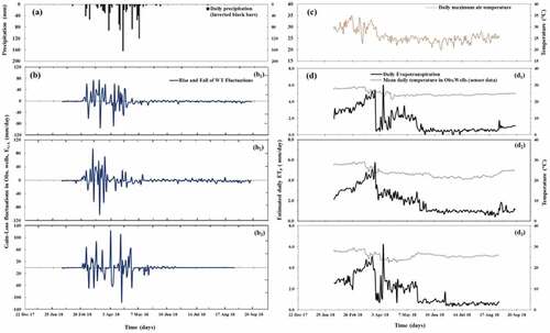
The periodic behavior of groundwater level fluctuations in TOWs in three SDs was primarily found to be a response to local ET, precipitation and water abstraction. Seasonal variations of water levels and temperatures in TOWs are presented in the supplemental Figure S8 and summarized in Figure 11 (b). These variations were found to follow the seasonality of rainfall pattern of the region (Figure 11 a). In general, water-level elevations in the alluvial sand-dam aquifers were found to decrease with increasing ET and Q_A till they become completely dry towards the end of September (see Figure 12 c).

Figure 11. Seasonal variation of (a) rainfall and (b) water table fluctuations in observation wells: S1 (b₁), S2 (b₂) and S3 (b₃) during the study period.

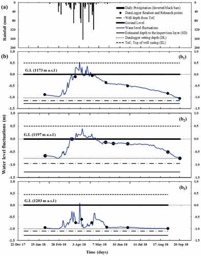
Figure 12. Field views of the temporary observation well at the site S1 during: (a) flood events), (b) the flood recession phase, and (c) the long dry season.

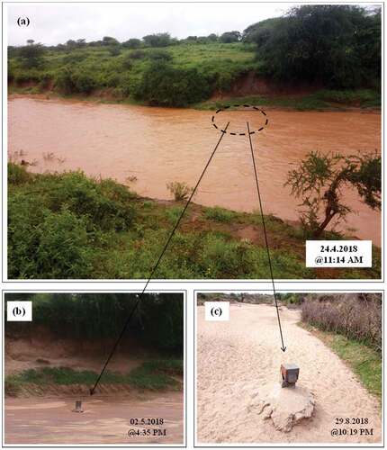
The Figure 11 b shows that water levels rose to the maximum during the rainy season (March-May 2018). Water level rose at 0.531 m (S1), 0.396 m (S2) and 0.073 m (S3) above the ground level. This was a result of heavy rainfall in April 2018 that produced heavy seasonal river floods, which, in turn, induced excess pressure heads above data loggers in the TOWs. Figure 12 (a) shows that the TOW was fully flooded and this means that water column thicknesses above the sensor tips of data loggers were very high. These artesian conditions of TOWs made data loggers inside the wells to record high water pressure values that produced high water levels. After floods recede (see Figure 12 (b), the artesian conditions stopped and water levels started becoming normal till sand-dam aquifers became completely dry (see Figure 12 (c)). The comparison of the three groundwater level patterns (see Figure 11. b) revealed that the SD (S3) does not retain harvested rainwater for a long period after the rainfall period (Figure 11 b₃). It was the first to become completely dry earlier in June 2018. This was because it is shallower (depth of 0.31 ± 0.19 m, 0–0.7 m) than the two remaining with mean depths of 0.74 ± 0.53 m (0–2.1 m) in SD (S1) and 0.46 ± 0.44 m (0–1.7 m) in SD(S2), respectively. Its mean sediment depth of 0.31 m was below 0.6 m which is considered as an effective depth below which SD systems can resist evaporative losses (Hellwig, 1973; Quinn, Parker, Rushton 2018). The SD (S1) with mean sediment depth of 0.74 m (> 0.6 m) was found to be likely able to alleviate the impact of evaporation losses. Finally, as it can be noticed from Figure 11 (c), there is a noticeable effect of lateral flow of external water intrusion into wellfield area on the normal water-level decline pattern. The field observation showed that there was an entry of wastewater from the the nearest residential area.

3.3. Water balance analysis results

3.3.1. Rainfall and runoff volumes

The three experimental SDs, respectively, received total seasonal rainfall/runoff volumes of about 62.13/36.21) million m³ in SD (S1), 4.11/2.39 million m³ in SD (S2), and 2.62/1.57 million m³ in SD (S3), resulting from the corresponding catchment areas of 7,416.47 ha, 480.34 ha and 306.41 ha respectively (see Table 7, Figure 13 and supplemental Figure S2). Both rainfall and runoff volumes correlated with polynomial regression coefficients higher than 0.98 (see supplemental Figure S9). The resulted runoff coefficient was in the order of arid and semiarid rangelands (0.59 ± 0.01) as described in the supplemental Table S2).

Figure 13. Potential runoff-contributing catchment areas (PRCAs) for the three experimental SDs (S1, S2 and S3).

Curve numbers for three delineated PRCAs were found to be, on average, 85.67 ± 0.47. This means that that these catchments (Figure 13) are of group C soils with a moderately high runoff potential. The major catchment characteristics are summarized in Table 7.

3.3.2. Recharge, discharge, and water loss fluxes

SD systems form unconfined aquifers after rainy seasons, and hydraulic heads within sediments fluctuate freely in response to changes in recharge and discharge (Figure 14 b). This Figure 14. b shows the seasonal variation of the water table exchange flux (E_GL) around the water table with respect to the rainfall pattern (Figure 14 a). Range and mean values of recharge and discharge fluxes in three SDs were, respectively, found to be 0.12–77.55 (12.09 ± 20.1) mm/day and 0.25–93.57 (5.82 ± 12.66) mm/day. In SD (S2), they were 0.00–92.16 (9.16 ± 16.34) mm/day and 0.24–102.24 (5.35 ± 11.94) mm/day. In SD (S3), they were 0.00–123.12 (13.21 ± 25.40) and 0.24–116.16 (6.79 ± 17.15) mm/day. In addition, as deducible from Figure 14 d, the range and mean values of evaporation rates were found to be 0.00–5.3 (1.54 ± 1.3) mm/day, 0.42–5.34 (1.88 ± 1.11 mm/day and 0.31–5.77 (1.69 ± 1.25) mm/day, respectively. These evaporation estimates were found to be in agreement with those estimated in the study of Quinn, Parker, et al. (2018).

Figure 14. Seasonal variations of water-table exchange fluxes in SD aquifers: (a) rainfall pattern, (b) water gain and loss fluxes; (c) maximum daily air temperature; (d) mean temperature and evaporation losses in observation wells S1, S2 and S3.

3.3.3. Synthesis of water balance components

In semi-arid and arid regions, the riverbeds carry the flood water only when erratic rainfall occurs. Therefore, the WBCs were estimated using Equation (8)(8) $R_E=Q_A+E_V+P_L+\mathrm{\Delta }{S}_D$(8) built on the presumption that no water is transported out of the SD system as subsurface flow beneath dry riverbeds. Rather, the lateral inflow and outflow as seepage exchanges would be expected to occur in the system. On this background knowledge, the monthly estimates of WBCs were carried out on a seasonal basis for the period of study from February to September 2018. Mean, minimum and maximum vertical hydraulic heads in TOWs indicated the seasonal variation of WBC estimates in both decline and depletion trends (Figure 15 b) with respect to the seasonal rainfall (Figure 15 a). Water balance analysis results are summarized in Table 8 and detailed WBC computations are presented in the supplemental Table S11.

Figure 15. Seasonal cycle of (a) long-rains season, (b) water balance estimates and hydraulic heads for three sites S1 (b1), S2 (b2) and S3 (b3) during the study period.

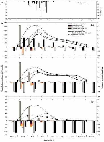
Figure 15 (b) shows the general overview of seasonal and monthly patterns of water balance estimates and water levels during the study period. These results showed that the three experimental SDs managed to harvest rainwater of about 5,801.50 m³ (S1) for an estimated water demand of 4,376.19 m³, 651.29 m³ (S2) for 1,883.70 m³, and 903.40 m³ (S3) for 2,730 m³ as indicated in Table 8 and Figure 16. Looking at these numbers, only the SD at the site S1 was likely to meet water demand as the harvested amount was higher than the demanded one. This was not the case because of water losses. The total water loss at SD (S1) was 3,318.15 m³ including evaporation and seepage losses of 2,229.96 m³ and 1,088.19 m^3, respectively. At the two other sites, evaporation (seepage) losses were estimated to be 441.52 (300.43) m³ in SD (S2) and 357.66 (387.40) m³ in SD (S3) as indicated in Table 8. Figure 16 shows that the SD (S3) exhibited the highest water loss (82.5%) compared to SD (S1) with 57.2% and SD (S2) with 67.8%. of its seasonal water storage.

Figure 16. Comparison of water savings and losses with water demand for the three sand-dam systems (S1, S2 and S3) in terms of (a) volumes and (b) percentages.

3.4. Performance analysis results

The performance analysis showed that if no water loss, the overall water demand satisfaction would have been rated as 81.83% (see Figure 17). On the contrary, after all losses, water demand satisfaction was rated as 31.72%. Overall performance indicators are summarized in Table 9. The studied SDs achieved very low stormwater capture efficiencies (SCE) of about 3.09 ± 1.98% due to their limited storage capacities. This value is in agreement with SCE values (1–3%) often reported in the literature (Hut et al., 2008; Maddrell & Neal, 2012; Neal, 2012; Quinn et al., 2019). In addition, they also achieved a low water-storage efficiency (WSE) of 30.85 ± 12.70% compared to other RWH systems that can achieve WSE levels of about 50 to 80% (Hofman & Paalman, 2014; Karim et al., 2014; Vargas et al., 2019). The temporal and volumetric reliabilities (R_T ad R_V) were found to be very undependable (see the last two rows of Table 9

Figure 17. Mass curves of cumulative harvested rainwater and water demand in three sand dams (S1, S2 & S3) during the study period.

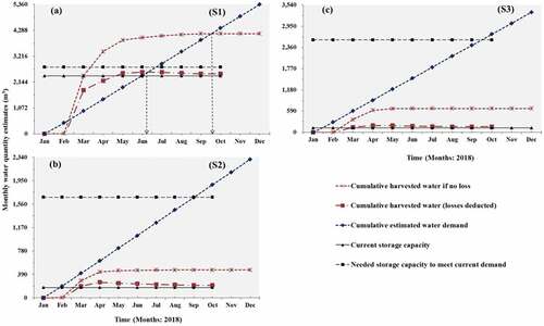
Table 8). Only SD (S1) exhibited good R_V (R_T) values of 56.75 (57.62) % compared to 11.14 (11.15) % for SD (S2) and 5.80 (5.95)%, respectively. This is because sediments accumulated in SD (S1) were moderately deep (0.74 ± 0.53 m: 0–2.05 m), wide (21–30 m: 26.22 ± 2.86 m) and reasonably porous (24.56 ± 4.88%) compared to the two remaining SDs (S2 and S3), with depths of 0.46 ± 0.44 (0–1.7 m) and 0.31 ± 0.19 m (0–0.75 m), respectively. As regards the water losses, evaporation was found to be the greatest threat to the performance of SD systems in dryland areas as it accounts for about 61.1% (±11.3) of total water losses. This finding is in agreement with the previous findings of Ngugi et al. (2020), De Trincheria et al. (2015a), Viducich (2015), and Eisma and Merwade (2020), who, respectively, reported that up to 58%, 80%, 50–67% and 51–85% of water storages in SDs are lost due to local ET. Water yield and demand curves (see Figure 17) showed that SD systems behave as conventional surface dams as they hold water for the period running from 2 weeks up to 3 months after the rainy season. Thus, SDs may be considered as subsistence water supply systems. Nevertheless, they are very important as the little they provide saves lives.

3.5. Water quality analysis results

The physicochemical and microbiological parameters obtained from analysis of water samples taken from scoop holes (SCHs, n = 31) and shallow wells (SHWs, n = 5) are presented in Table 10. These results showed that water from SD systems, either via scoop holes or shallow wells, should not be directly consumed before being treated by either chlorination or boiling. This is because the overall microbiological non-compliance rates with the KEBS limit of 0 CFU/100 ml were 90.79% (total coliforms, TCs) and 35.13% (Escherichia coli, E.coli) in scoop holes, and 60% (TCs) in shallow wells. The presence of TCs at these rates is an indication that water abstracted from SD systems is vulnerable to microbial contamination. This finding is, to some extent, in agreement with previous findings (Abila et al., 2012; Onyango et al., 2018; Quinn et al., 2018), (Graber Neufeld et al., 2020; Onyango-Ouma & Gerba, 2011). It was observed that scoop holes are more vulnerable to contamination than shallow wells because they are easily accessible to the public and animals (see See the supplemental Figure S10 a). Pathogens from animal wastes and other dissolved contaminants can diffuse into SD sands through scoop holes left open to air (see Figure S10 a) or through the natural porosity of sandy sediments. As regards the physicochemical quality, the computed water pollution indices (see the last row and column of Table 10) showed that the sand-dam water is unsuitable for drinking purposes. Water abstracted via scoop holes was, on average, rated as “Polluted” as it scored a WPI of 12.90 > 1 (Best water, clean water). Water from shallow wells was found to be fairly clean (WPI = 1.86 > 1) as they are protected from direct contact with contaminants (See Figure S10 (e,f)).. The WPI results are in agreement with field observations because water from scoop holes looked muddy during some weeks after rainfall and became slightly clear in the later period. On average, scoop-hole water has a higher turbidity level of 393.6 NTU (> 25 NTU (KEBS limit) and > 5 NTU (WHO limit) compared to the shallow-water with a low turbidity level of about 1.4 NTU < 25 NTU and <5 NTU.

In addition, by having a glance at Table 10, one can see that the turbidity and iron in scoop holes have high WPI values of about 15.72 and 9.72, respectively. This indicates that muds and iron have a great influence on the sand-dam water color and can make it objectionable for esthetic reasons. Although the turbidity may not cause harm and threat to the life of sand-dam water users, some microbial germs may cling to sediment particles and these germs may lead to devastating waterborne diseases. The problem of water turbidity can be solved by treating the fetched water at households using local methods such as sand-charcoal filters, settling and decanting containers, biosand filters, bucket filters, ceramic filters, and porous pot filters, etc. Some studies proved that these methods are more effective in reducing turbidity and other chemical pollutants (Mwabi et al., 2011). This turbidity removal process can be supplemented by water chlorination with disinfection byproducts (DBPs) available in the local market to kill potential pathogens. Knowing that the continuous use of DBPs can lead to potential health risks of developing certain cancers like bladder, colon, and rectal cancers ((Ashbolt, 2004; Evans et al., 2020; Hamidin et al., 2008; Singer, 1994), the use of DBPs may be balanced with other methods that kill microbes like water boiling, and solar water disinfection (SODIS).

4. Conclusions

The results from the present study showed that the three investigated sand dams (SDs) poorly performed their primary functions, namely, providing adequate water of good quality, and protecting stored water from contamination and evaporation losses. They exhibited low operational efficiencies due to their limited water-storage capacities, high evaporation losses, and high inter-seasonal climate variability. Their water-storage capacity was found to be a function of volumes and depths of accumulated sands, hydraulic geometry, gradation and specific yield of these sands. Evaporation water losses were found to be of significant concern and a great threat to the effectiveness of SD systems as they constituted more than half of the total water losses. As regards to water quality, some major physicochemical and microbiological properties (mainly turbidity, iron, Escherichia coli and total coliforms) do not meet both WHO and KEBS water quality guidelines. Water extracted via scoop holes was found to be of poor quality and high vulnerability to contamination compared to that of shallow wells. The study suggests that there is a potential risk of contracting waterborne diseases and other health ailments. Therefore, this calls for the necessity to disinfect all water fetched from SD systems regardless of the method used to fetch it. As a result of the present study limitations, future studies should assess: (a) long-term effects of human and livestock traffics over sand aquifers on water quality and associate the latter with the local and regional morbidity from waterborne diseases; and (b) long-term effects of sand harvesting on storage capacities of sand dams and their overall performance.

Acknowledgements

This work was supported by the African Union Commission (AUC) research grant as part of the Pan-African University Scholarship. We owe a big thanks to Aqualytic Laboratories Limited (Kenya), for providing water quality testing kits and water analysis services. We would like to express our gratitude to Fredrick K. Mbiti and Bosco M. Lonzi for their support in data collection and transport. We owe special thanks to Lusia M. Mwanzia for having kept an eye on research materials during the whole period of study, and to anonymous reviewers for their constructive comments to improve this article.

Disclosure statement

No potential conflict of interest was reported by the authors.

Supplementary material

Supplemental data for this article can be accessed online at https://doi.org/10.1080/23311916.2022.2163572

Additional information

Notes on contributors

Moïse Ndekezi

Moïse Ndekezi is currently a PhD Candidate in Civil Engineering (Environmental and Arid and Semi-arid Lands Engineering) at Pan-African University Institute for Basic Sciences, Technology and Innovation (PAUSTI), Kenya. He has 10 years of experience in civil engineering, particularly in water resources engineering, both in teaching career and professional practice. He earned his Bachelor’s degree in civil engineering and environmental technology in 2011 from the former Kigali Institute of Science and Technology (KIST), currently the College of Science and Technology, University of Rwanda (UR-CST). He is currently an assistant lecturer at the same college in the Department of Civil, Environmental and Geomatics Engineering. He earned a joint Master’s degree in water resources engineering in 2014 from Katolieke Universiteit Leuven (KU Leuven) and Vrije Universiteit Brussel (VUB), Belgium. Since 2021, he is a fully-fledged member of Institution of Engineers Rwanda (IER) and member of the National Technical Advisory Committee (NTAC) on Construction and Use of Dams. His research interests focus on sustainability of water storage systems, reservoir sedimentation and sediment management strategies, advanced irrigation and drainage systems, groundwater hydraulics and pollutant transport, watershed and flood modeling, urban hydraulics and stormwater management, water quality monitoring, climate change mitigation and adaptation strategies.

References

- Abila, R., Muthangya, M., Mutuku, E., Mutati, K., Munguti, M., & Musyoka, C. M. (2012). Physico-chemical and bacteriological quality assessment of shallow wells in Kitui town, Kenya. Journal of Environmental Science and Water Resources, 1(2), 27–41. https://ir-library.mmarau.ac.ke:8080/bitstream/handle/123456789/2564/Prof%20Abila%201.pdf
- Aboelnga, H. T., Ribbe, L., Frechen, F.-B., & Saghir, J. (2019). Urban water security: Definition and assessment framework. Resources, 8(4), 1–19. https://doi.org/10.3390/resources8040178
- Aerts, J., Lasage, R., Beets, W., de Moel, H., Mutiso, G., Mutiso, S., & de Vries, A. (2007). Robustness of sand storage dams under climate change. Vadose Zone Journal, 6(3), 572–580. https://doi.org/10.2136/vzj2006.0097
- Allen, R. G., Pereira, L. S., Raes, D., & Smith, M. (1998). Annex 2. Meteorological tables. In Crop evapotranspiration - Guidelines for computing crop water requirements. Rome, Italy: Food and Agriculture Organization of the United Nations (FAO Irrigation and drainage paper 56). http://www.fao.org/3/X0490E/x0490e0j.htm.
- Anovitz, L. M., & Cole, D. R. (2015). Characterization and analysis of porosity and pore structures. Reviews in Mineralogy and Geochemistry, 80(1), 61–164. http://dx.doi.org/10.2138/rmg.2015.80.04
- Anton, D. K., & Shelton, D. L. (2011). Environmental protection and human rights. Cambridge University Press.
- Aquaveo. (2016). WMS 10.1 Tutorials: Watershed Modeling – DEM Delineation. Aquaveo, LLC (environmental and water resources modeling software company) (WMS 10.1) http://wmstutorials-10.1.aquaveo.com/7%20WatershedModeling-DEMDelineation.pdf [Accessed 20 January 2018]
- Ashbolt, N. J. (2004). Risk analysis of drinking water microbial contamination versus disinfection by-products (DBPs). Toxicology, 198(1–3), 255–262. https://doi.org/10.1016/j.tox.2004.01.034
- Balugani, E., Lubczynski, M. W., & Metselaar, K. (2016). A framework for sourcing of evaporation between saturated and unsaturated zone in bare soil condition. Hydrological Sciences Journal, 61(11), 1981–1995. https://doi.org/10.1080/02626667.2014.966718
- BSI. (2002). Specification for aggregates from natural sources for concrete. Concrete Aggregates guideline (BS 882:1992). British Standards Institution (BSI) British Standards Institution. Accessed 20 March, 2018: http://www.c-s-h.ir/wp-content/uploads/2015/10/BS-882.pdf
- Butler, D., & Memon, F. A. (eds.). (2006). Water demand management. IWA Publishing. https://doi.org/10.2166/9781780402550
- Das, B. M. (2002). Soil Mechanics Laboratory Manual. 6th ed. Oxford University Press. http://site.iugaza.edu.ps/dsafi/files/2015/02/Soil-Laboratory-Manual-Das.pdf [Accessed 12 May 2018]
- De Leeuw, J., Njenga, M., Wagner, B., & Liyama, M., eds. (2014). Treesilience: an assessment of the resilience provided by trees in the drylands of Eastern Africa. World Agroforestry Centre (ICRAF). http://www.worldagroforestry.org/downloads/publications/PDFs/B17611.PDF [Accessed 12 May 2020]
- De Trincheria, J., Nissen-Petersen, E., Filho, L. W., & Otterphol, R. (2015a). Factors affecting the performance and cost-efficiency of sand storage dams in South-Eastern Kenya. In Proceedings of the 36th IAHR World Congress, 28 June – 3 July, 2015. The Hague, the Netherlands. IAHR Document Library. https://www.iahr.org/library/info?pid=7777.
- Doreau, M., Corson, M. S., & Wiedemann, S. G. (2012). Water use by livestock: A global perspective for a regional issue? Animal Frontiers, 2(2), 9–16. https://doi.org/10.2527/af.2012-0036
- Du Plessis, A. (2019). Current and future water scarcity and stress. In water as an inescapable risk: Current global water availability, quality and risks with a specific focus on South Africa;Springer. Ch: 1. pp.13-25. https://doi.org/10.1007/978-3-030-03186-2_2
- Effendi, H., Wardiatno, Y., & Wardiatno, Y. (2015). Water quality status of ciambulawung river, banten province, based on pollution index and NSF-WQI. Procedia Environmental Sciences, 24, 228–237. https://doi.org/10.1016/j.proenv.2015.03.030
- Eisma, J. A., & Merwade, V. M. (2020). Investigating the environmental response to water harvesting structures: A field study in Tanzania. Hydrology and Earth System Sciences Discussions, 24(4), 1891–1906. https://doi.org/10.5194/hess-24-1891-2020
- Eisma, J. A., Saksena, S., & Merwade, V. (2021). Assessing the impact of land cover, soil, and climate on the storage potential of dryland sand dams. Frontiers in Water, 3(671455). https://doi.org/10.3389/frwa.2021.671455
- Ertsen, M. W., Biesbrouck, B., Postma, L., & van Westerop, M. (2005). Community organisation and participatory design of sand-storage dams in Kenya. In T. Goessling, R. J. G. Jansen, & L. A. G. Oerleman (Eds.), Coalitions and collisions (pp. 175–185). Wolf Publishers.
- Evans, S., Campbell, C., & Naidenko, O. V. (2020). Analysis of cumulative cancer risk associated with disinfection byproducts in united states drinking water. International Journal of Environmental Research and Public Health, 17(6), 2149. https://doi.org/10.3390/ijerph17062149
- FEWS, N. E. T. (2019). Kenya food security outlook update. Situation report (August 2019). USAID Famine Early Warning Systems Network. https://reliefweb.int/sites/reliefweb.int/files/resources/KENYA_Food_Security_Outlook_Update_August2019_Final.pdf [Accessed 12 November 2019].
- Fitts, C. R. (2002). Deformation, storage, and general flow equations. In Groundwater Science 1st. Elsevier Science Ltd. Ch; 125–65. https://booksite.elsevier.com/9780122578557/PDFs/Ch_5.pdf Accessed 20 March 2018
- Flintan, F., Behnke, R., & Neely, C. (2013). Natural resource management in the drylands in the Horn of Africa. Technical Consortium Brief. Nairobi: International Livestock Research Institute Technical Consortium partnership between CGIAR and the FAO Investment Centre. https://dlci-hoa.org/assets/upload/key-resilience-and-climate-change/20200803113921946.pdf [Accessed 12 May 2020]
- Gladys, K. V. (2017). Rainfall and temperature variability and its effect on food security in Kitui county, Kenya. International Journal of Development and Sustainability, 6(8), 924–939. https://isdsnet.com/ijds-v6n8-29.pdf
- GoK. (2012). Vision 2030 Development Strategy for Northern Kenya and Other Arid Lands. A policy report. Nairobi: Government of the Republic of Kenya. http://extwprlegs1.fao.org/docs/pdf/ken179242.pdf [Accessed 12 March 2018]
- GoK. (2019). Drought situation & early warning phase classification in Kitui County. Situation Report, Drought Early Warning Bulletin for November 2019. National Drought Management Authority (NDMA). https://www.ndma.go.ke/index.php/resource-center/send/26-kitui/5449-kitui-november-2019.pdf [Accessed 20 January 2020].
- GoK. (2020). Drought Situation & Early Warning Phase Classification in Kitui County. Situation report, Early Warning Bulletin for September 2020. National Drought Management Authority (NDMA). https://www.ndma.go.ke/index.php/resource-center/send/26-kitui/5788-kitui-september-2020 [Accessed 12 November 2020]
- Graber Neufeld, D., Muendo, B., Muli, J., & Kanyari, J. (2020). Coliform bacteria and salt content as drinking water challenges at sand dams in Kenya. Journal of Water and Health, 18(4), 602–612. https://doi.org/10.2166/wh.2020.192
- Guo, J. C., & Urbonas, B. (1996). Maximized detention volume determined by runoff capture ratio. Journal of Water Resources Planning and Management, 122(1), 33–39. https://doi.org/10.1061/(ASCE)0733-9496(1996)122:1(33)
- Hach. (2012). Water Analysis Handbook. 7th ed.: Hach Company. http://www.prosess-styring.no/nedlasting/prosman/dr6000/WAH_2012/DOC086.52.01000.pdf [accessed 16 August 2018]
- Hamidin, N., Yu, Q. J., & Connell, D. W. (2008). Human health risk assessment of chlorinated disinfection by-products in drinking water using a probabilistic approach. Water Research, 421, 3263–3274. Water research. https://doi.org/10.1016/j.watres.2008.02.029
- Hanson, L. S., & Vogel, R. M. (2014). Generalized storage–reliability–yield relationships for rainwater harvesting systems. Environmental Research Letters, 9(7), 1–10. https://doi.org/10.1088/1748-9326/9/7/075007
- Harter, T. (2005). Specific yield storage equation. In Water encyclopedia J. H. Lehr & J. Keeley Eds. John Wiley & Sons, Inc. Ch 576–78. https://doi.org/10.1002/047147844X.gw1086
- Hellwig, D. H. R. (1973). Evaporation of water from sand, 4: The influence of the depth of the water-table and the particle size distribution of the sand. Journal of Hydrology, 18(3–4), 317–327. https://doi.org/10.1016/0022-1694(73)90055-3
- Hofman, J. A. M. H., & Paalman, M. (2014). Rainwater harvesting, a sustainable solution for. KfC report No.KfC 142/2014. National Research Programme Knowledge for Climate. https://edepot.wur.nl/345625 [ Accessed 12 May 19].
- Hoogmoed, M. (2007). Analyses of impacts of a sand storage dam on groundwater flow and storage: Groundwater flow modelling in Kitui District, Kenya. [ Msc Thesis]. Vrije Universiteit Amsterdam. http://www.samsamwater.com/projects/46/data/Hoogmoed_-_2007_-_Analyses_of_impacts_of_a_sand_storage_dam_on_gw_flow_and_storage_0.pdf [Accessed 17 January 2017].
- Hussey, W. S. (2007). Water From Sand Rivers: Guidelines for abstraction. Water, Engineering and Development Centre (WEDC), Loughborough University, UK. https://wedc-knowledge.lboro.ac.uk/resources/books/Water_From_Sand_Rivers_-_Complete.pdf [Accessed 19 April 2018]
- Hut, R., Ertsen, M., Joeman, N., Vergeer, N., Winsemius, H., & van de Giesen, N. (2008). Effects of sand storage dams on groundwater levels with examples from Kenya. Physics and Chemistry of the Earth, Parts A/B/C, 33(1), 56–66. https://doi.org/10.1016/j.pce.2007.04.006
- Jama, B., & Zeila, A., 2005. Agroforestry in the drylands of Eastern Africa: A call to action. ICRAF Working Paper – No.1. Nairobi: World Agroforestry Centre. http://www.worldagroforestry.org/downloads/publications/PDFs/wp05043.pdf [12 May 2020].
- Jenkins, M. W., Tiwari, S. K., & Darby, J. (2011). Bacterial, viral and turbidity removal by intermittent slow sand filtration for household use in developing countries: Experimental investigation and modeling. Water Research, 45(18), 6227–6239. https://doi.org/10.1016/j.watres.2011.09.022
- Kalungu, J. W., Walter, L. F., Mbuge, D. O., & Cheruiyot, H. K. (2015). Assessing the impact of rainwater harvesting technology as adaptation strategy for rural communities in Makueni County, Kenya. In L. F. Walter (Ed.), Handbook of Climate Change Adaptation (pp. 1615–1634). Springer.
- Karim, M. R., Rimi, R. A., & Billah, M. S. 2014. Analysis of storage volume and reliability of the rainwater harvesting tanks in the coastal area of Bangladesh. Desalination and Water Treatment, 54(13), 3544–3550. https://doi.org/10.1080/19443994.2014.923201.
- KEBS. (2015). Kenya Standard (KS EAS 12: 2014, First Edition)_Specifications for potable water. Reference No.G/TBT/N/KEN/470. Kenya Bureau of Standards Kenya Bureau of Standards. http://www.puntofocal.gov.ar/notific_otros_miembros/ken470_t.pdf [Accessed 18 April 2018]
- Kenya Ministry of Health. (2017. Sanitation Profile for Kitui County. Information fact sheet. Nairobi, Kenya: Ministry of Health, Republic of Kenya, in partnership with the World Bank Group and the United Nations Children’s Fund. http://sanitationandwaterforall.org/wp-content/uploads/download-manager-files/Kitui.pdf [Accessed 28 February 2018]
- Kitheka, J. U. (2016). Seasonal river channel water exchange and implications on salinity levels in sand dams: Case of semi-arid Kitui Region,Kenya. Journal of Environment and Earth Science, 6(12), 66–85. https://www.iiste.org/Journals/index.php/JEES/article/view/34568/35571
- Kra, E. (2014). FAO-56 penman-monteith daily E T o from linear regression calibrated hargreaves equation with wind terms in tropics with limited data. International Journal of Agronomy, 2014, 1–9. https://doi.org/10.1155/2014/402809
- Lasage, R., Aerts, J., Mutiso, G.-C. M., & De Vries, A. (2008). Potential for community based adaptation to droughts: Sand dams in Kitui, Kenya. Physics and Chemistry of the Earth, 33(1), 67–73. https://doi.org/10.1016/j.pce.2007.04.009
- Lasage, R., Aerts, J. C., Verburg, P. H., & Sileshi, A. S. (2015). The role of small scale sand dams in securing water supply under climate change in Ethiopia. Mitigation and Adaptation Strategies for Global Change, 20(2), 317–339. https://doi.org/10.1007/s11027-013-9493-8
- Lasage, R., & Andela, N. (2011). Impact of sand dams and climate change on modelled discharge. Dawa river basin, Ethiopia. IVM report (R-11/01a). Institute for Environmental Studies (IVM) VU University. https://research.vu.nl/ws/portalfiles/portal/3052400/R11-01.pdf [Accessed 20 April 2018].
- Lasage, R., Pauw, W. P., Aerts, J. C., Mutiso, S., Mutiso, G., De Vries, A., & Manzi, H. K. (2008). An assessment of the social and economic effects of the kitui sand dams. Research report No. R-08/08. Sahel Solutions (SASOL) & Institute for Environmental Studies (IVM) Vrije Universiteit. https://research.vu.nl/ws/portalfiles/portal/2415504/R-08-08.pdf [Accessed 18 February 2018].
- Lasage, R., & Verburg, P. H. (2015). Evaluation of small scale water harvesting techniques for semi-arid environments. Journal of Arid Environments, 118, 48–57. https://doi.org/10.1016/j.jaridenv.2015.02.019
- Leal Filho, W., & De Trincheria, G. J. (eds.). (2018). Rainwater-smart agriculture in arid and semi-arid areas: Fostering the use of rainwater for food security, poverty alleviation, landscape restoration and climate resilience. Springer. https://doi.org/10.1007/978-3-319-66239-8
- Maddrell, S. (2013). Sand dams: A sustainable solution for rural drylands. In USAID workshops on sand dams & climate change. Excellent Development Ltd. https://doi.org/10.13140/RG.2.2.25054.13123
- Maddrell, S. (2016). Securing water supplies with sand dams. Ingenia, 66, 26–32. https://www.ingenia.org.uk/getattachment/d46e994c-daa6-4cf1-ab39-cc6ca742d313/maddrell.pdf
- Maddrell, S., & Neal, I. (2012). Sand dams: a Practical Guide. Excellent Development Ltd. https://www.samsamwater.com/library/Maddrell_and_Neal_2012_Sand_Dams_a_Practical_Guide_LR.pdf [Accessed 11 March 2018]
- Maddrell, S., & Neal, I. (2013). Building sand dams: a practical guide. Practical Guide. Excellent Development Ltd. http://www.rainfoundation.org/wp-content/uploads/2017/10/Sand-Dam-Manual-Version-2-review-copy-1.pdf [Accessed 16 May 2018]
- Mancosu, N., Snyder, R. L., Kyriakakis, G., & Spano, D. (2015). Water scarcity and future challenges for food production. Water, 7(3), 975–992. https://doi.org/10.3390/w7030975
- Manzi, H. K., & Kuria, D. N. (2011). The use of satellite images to monitor the effect of sand dams on stream bank land cover changes in Kitui District. Journal of Agriculture, Science and Technology, 13(2). https://journals.jkuat.ac.ke/index.php/jagst/article/download/606/557
- Matko, V. (2003). Porosity determination by using stochastics method. Automatika: Journal for Control, Measurement, Electronics, Computing and Communications, 44(3–4), 155–162. https://hrcak.srce.hr/file/10210
- McCabe, G. J., & Wolock, D. M. (2016). Variability and trends in runoff efficiency in the conterminous United States. Journal of the American Water Resources Association (JAWRA), 52(5), 1046–1055. https://doi.org/10.1111/1752-1688.12431
- McGrath, T. J., Morrison, P. D., Ball, A. S., & Clarke, B. O. (2018). Detection of novel brominated flame retardants (NBFRs) in the urban soils of Melbourne, Australia. Emerging Contaminants, 3(1), 23–31. https://doi.org/10.1016/j.emcon.2017.01.002
- Moriasi, D. N., Gitau, M. W., Pai, N., & Daggupati, P. (2015). Hydrologic and water quality models: Performance measures and evaluation criteria. Transactions of the ASABE, 58(6), 1763–1785. https://doi.org/10.13031/trans.58.10715
- MoWI. (2015a). Practice Manual For Small Dams, Pans and Other Water Conservation Structures in Kenya. 2nd ed. State Department for Water, Ministry of Water and Irrigation, Government of Kenya. http://smalldamsguidelines.water.go.ke/useful_downloads/pdf/PRACTICE_MANUAL_FOR_SMALL_DAMS_PANS_AND_OTHER_WATER_CONSERVATION_STRUCTURES_IN_KENYA.pdf [Accessed 10 May 2018]
- MoWI. (2015b). Practice manual for small dams, pans and other water conservation structures in Kenya. Manual. State Department for Water, Ministry of Water and Irrigation Ministry of Water and Irrigation, Government of Kenya. http://smalldamsguidelines.water.go.ke/useful_downloads/pdf/PRACTICE_MANUAL_FOR_SMALL_DAMS_PANS_AND_OTHER_WATER_CONSERVATION_STRUCTURES_IN_KENYA.pdf Accessed 12 January 2018
- Mutati, K., Kitheka, J. U., & Otieno, E. (2018). Sand gradation in seasonal rivers and their suitability for construction of sand dams in Kitui South, Kenya. Hydrology: Current Research, 9(1), 295. https://doi.org/10.4172/2157-7587.1000295
- Muthini, A. D., Munguti, K. K., Appleford, G., Odero, V., Wendy, E., Swai,& Annmarie. (2014). Tapping water resources and their potential in the arid and semi arid lands: The case of marsabit county, Kenya. A casestudy report. Concern Worldwide. https://reliefweb.int/sites/reliefweb.int/files/resources/concern_water_study_final.pdf [Accessed 10 January 2019].
- Mutiso, S. K., & Thompson, R. D. (1987). Future water supply in the Machakos District of Kenya. Ambio, 16(6), 322–325. https://www.jstor.org/stable/4313394
- Mutunga, E. J., Ndungu, C. K., & Muendo, P. (2018). Factors influencing smallholder farmers’ adaptation to climate variability in Kitui County, Kenya. International Journal of Environmental Sciences & Natural Resources, 8(5). https://doi.org/10.19080/IJESNR.2018.08.555746
- Muyanga, M., & Mutua, I. (2000). From rhetoric to practice, gender participation in the fight for survival: The story of sand dams in Kitui (Kenya). Case study report No. 202.1-17294. International Water and Sanitation Centre (IRC). https://www.ircwash.org/sites/default/files/202.1-17294.pdf [Accessed 12 April 2019].
- Mwabi, J. K., Adeyemo, F. E., Mahlangu, T. O., Mamba, B. B., Brouckaert, B. M., Swartz, C. D., Offringa, G., Mpenyana-Monyatsi, L., & Momba, M. N. B. (2011). Household water treatment systems: A solution to the production of safe drinking water by the low-income communities of Southern Africa. Physics and Chemistry of the Earth, Parts A/B/C, 36(14–15), 1120–1128. https://doi.org/10.1016/j.pce.2011.07.078
- Mwamati, F. T., Kitheka, J. U., & Njuru, G. P. (2017). An assessment of the spatial and temporal variations of groundwater quality in Yatta Plateau in Kitui County, Kenya. Journal of Environment and Earth Science, 7(1), 90–104. https://www.iiste.org/Journals/index.php/JEES/article/view/34995/35995
- Neal, I. (2012). The potential of sand dam road crossings. Dams and Reservoirs, 22(3–4), 129–143. https://dx.doi.org/10.1680/dare.13.00004
- Ngugi, K. N. K., Gichaba, M. C. M., Kathumo, V. V. M., & Ertsen, M. M. W. (2020). Back to the drawing board: Assessing siting guidelines for sand dams in Kenya. Sustainable Water Resources Management, 6(4), 1–28. https://doi.org/10.1007/s40899-020-00417-4
- Njoka, J. T., Yanda, P., Maganga, F., Liwenga, E., Henku, A., Kateka, A., Mabhuye, E., Malik, N., & Bavo, C. (2016). Kenya: Country situation assessment. Working paper. Nairobi: Pathways to Resilience in Semi-arid Economies (PRISE). Center for Sustainable Dryland Ecosystems and Societies (CSDES). http://prise.odi.org/wp-content/uploads/2016/01/Low-Res_Kenya-CSA.pdf [Accessed 14 February 2018].
- NRCS. (1986). Urban Hydrology for Small Watersheds. Technical Release 55 (TR-55). United States Department of Agriculture Natural Resources Conservation Service. https://www.nrcs.usda.gov/Internet/FSE_DOCUMENTS/stelprdb1044171.pdf [Accessed 17 March 2019]
- Ociepa, E., Mrowiec, M., & Deska, I. (2019). Analysis of water losses and assessment of initiatives aimed at their reduction in selected water supply systems. Water, 11(5), 1037. https://doi.org/10.3390/w11051037
- Onset Computer Corporation, 2008. Barometric Compensation Assistant (BCA), a post-processor designed for use with HOBOware Pro on the PC or Mac [White paper]. Bourne, United States: Onset Computer Corporation http://www.onsetcomp.com/files/support/tech-notes/onsetBCAguide.pdf [Accessed 20 March 2018].
- Onset Computer Corporation. (2018). HOBO U20L Water Level Logger (U20L-0x) Manual. Onset Computer Corporation: https://www.onsetcomp.com/files/manual_pdfs/17153-G%20U20L%20Manual.pdf [Accessed 2018 June 2018]
- Onyango, A. E., Okoth, M. W., Kunyanga, C. N., & Aliwa, B. O. (2018). Microbiological quality and contamination level of water sources in Isiolo County in Kenya. Journal of Environmental and Public Health, 2018, 1–10. https://doi.org/10.1155/2018/2139867
- Onyango-Ouma, W., & Gerba, C. P. (2011). Away-from-home drinking water consumption practices and the microbiological quality of water consumed in rural western Kenya. Journal of Water and Health, 9(4), 628–636. https://doi.org/10.2166/wh.2011.115
- Prăvălie, R. (2016). Drylands extent and environmental issues. A global approach. Earth-Science Reviews, 162, 259–278. https://doi.org/10.1016/j.earscirev.2016.08.003
- Quilis, R. O., Hoogmoed, M., Ertsen, M., Foppen, J. W., Hut, R., & Vries, A. D. (2009). Measuring and modeling hydrological processes of sand-storage dams on different spatial scales. Physics and Chemistry of the Earth, 4(Parts A/B/C 34), 289–298. https://doi.org/10.1016/j.pce.2008.06.057
- Quinn, R., Avis, O., Decker, M., Parker, A., & Cairncross, S. (2018). An assessment of the microbiological water quality of sand dams in Southeastern Kenya. Water, 10(6), 708. https://doi.org/10.3390/w10060708
- Quinn, R., Parker, A., & Rushton, K. (2018). Evaporation from bare soil: Lysimeter experiments in sand dams interpreted using conceptual and numerical models. Journal of Hydrology, 564, 909–915. https://doi.org/10.1016/j.jhydrol.2018.07.011
- Quinn, R., Rushton, K., & Parker, A. (2019). An examination of the hydrological system of a sand dam during the dry season leading to water balances. Journal of Hydrology X, 4, 100035. https://doi.org/10.1016/j.hydroa.2019.100035
- Rantz, S. E., 1982. Measurement and computation of streamflow, volume 1: Measurement of stage and discharge. US geological survey water supply paper 2175. Washington: United States Government Printing Office. https://pubs.usgs.gov/wsp/wsp2175/pdf/WSP2175_vol1a.pdf [Accessed 19 January 2018].
- Reed, B., & Reed, B. (2013). How much water is needed in emergencies? Technical Note No. WHO_TN_09. World Health Organization Loughborough University. https://www.who.int/water_sanitation_health/publications/2011/WHO_TN_09_How_much_water_is_needed.pdf [Accessed 12 June 2018]
- Ryan, C., & Elsner, P. (2016). The potential for sand dams to increase the adaptive capacity of East African drylands to climate change. Regional Environmental Change, 16(7), 2087–2096. https://doi.org/10.1007/s10113-016-0938-y
- Semanaz, S. P. (2018). The water crisis in Ethiopia and kenya: Being locked out of water and sanitation. Global Majority E-Journal, 9(2), 84–98. https://www.american.edu/cas/economics/ejournal/upload/perez_accessible.pdf
- Singer, P. C. (1994). Control of disinfection by‐products in drinking water. Journal of Environmental Engineering, 120(4), 727–744. https://doi.org/10.1061/(ASCE)0733-9372(1994)120:4(727)
- Smet, J., & van Wijk, C., eds. (2002). Small Community Water Supplies: Technology, People and Partnership. IRC International Water and Sanitation Centre. https://www.ircwash.org/sites/default/files/Smet-2002-Small_TP40.pdf [Accessed 14 May 2018]
- Song, J., & Chen, X. (2010). Variation of specific yield with depth in an alluvial aquifer of the Platte River valley, USA. International Journal of Sediment Research, 25(2), 185–193. https://doi.org/10.1016/S1001-6279(10)60037-6
- Soundharajan, B.-S., Adebayo, A. J., & Remesan, R. (2016). Evaluating the variability in surface water reservoir planning characteristics during climate change impacts assessment. Journal of Hydrology, 538(2016), 625–639. https://dx.doi.org/10.1016/j.jhydrol.2016.04.051
- Stern, J. H., & Stern, A. 2011. Water Harvesting through Sand Dams. ECHO Technical Notes, TN #70. ECHO, Inc. http://edn.link/nddxad [Accessed 12 May 2018]
- Studer, R. M., & Lininger, H. (2013). Water Harvesting: Guidelines to Good Practice. Geographica Bernensia. https://wocatpedia.net/images/4/4a/Water_Harvesting_Guidelines_to_Good_Practice.pdf [Accessed 22 April 2018]
- Suwandana, E., Kawamura, K., Sakuno, Y., & Raharjo, P. (2011). Evaluation of spatial distribution patterns of rivers and groundwater at different times in Jakarta, Indonesia using the water pollution index. Journal of the Japanese Agricultural Systems Society, 27(3), 91–102. https://doi.org/10.14962/jass.27.3_91
- Thomas, D. B. (1999). Where there is no water: A story of community water development and sand dams in Kitui District Kenya. Water development progress report No.824-KE-15676. Sahelian Solutions Foundation (SASOL). https://www.ircwash.org/sites/default/files/824-KE-15676.pdf [Accessed 15 April 2018].
- Van Dalen, D. B., de Wildt, S., & Muendo, B. (2018). Ensuring resilience through community sand dams in Kenya. https://gripp.iwmi.org/wp-content/uploads/sites/2/2018/08/WaterStorage_Kenya_SWWW2018.pdf [Accessed 22 August 2018]
- Van der Steen, C. (2015). Keeping on Keeping on: A realist perspective on the scale of sand storage dams in Kenya from 2005-2015. [ Msc Thesis] Wageningen University. http://edepot.wur.nl/364965 [Accessed: 28 February 2019].
- Vargas, D., Dominguez, I., Ward, S., & Oviedo-Ocañaa, E. R. (2019). Assisting global rainwater harvesting practitioners: A decision support tool for tank sizing method selection under uncertainty. Environmental Science: Water Research & Technology, 5(3), 506–520. https://doi.org/10.1039/c8ew00707a
- Viducich, J. M. G. (2015). Spillway Staging and Selective Sediment Deposition in Sand Storage Dams. [ Master’s thesis]. Oregon State University Graduate School. https://ir.library.oregonstate.edu/concern/parent/1z40kx51c/file_sets/vm40xw34c [Accessed 22 May 2018].
- Villani, L., Castelli, G., Hagos, E. Y., & Bresci, E. (2018). Water productivity analysis of sand dams irrigation farming in northern Ethiopia. Journal of Agriculture and Environment for International Development (JAEID), 112(1), 139–160. https://doi.org/10.12895/jaeid.20181.726
- Wandiga, S. O. (2015). Critical water issues in Africa. In S. Ahuja, J. B., De Andrade, D. D., Dionysiou, K. D., Hristovski, & B. G., Loganathan (Eds.), Water challenges and solutions on a global scale (pp. 95–113). American Chemical Society. Ch. https://doi.org/10.1021/bk-2015-1206.ch006
- WHO. (2003). General comment on the right to water. In The right to water. World Health Organization. pp.12–21. https://www.who.int/water_sanitation_health/en/righttowater.pdf [Accessed 20 May 2018]
- WHO. (2017). Guidelines for drinking-water quality: Fourth edition incorporating the first addendum. World Health Organization. https://apps.who.int/iris/bitstream/handle/10665/254637/9789241549950-eng.pdf?sequence=1 [accessed 19 March 2018]
- WHO/UNICEF. (2000). Global water supply and sanitation assessment 2000 report. World Health Organization. http://www.who.int/water_sanitation_health/monitoring/jmp2000.pdf [Accessed March 20, 2018]
- World Weather Online. (2019). Kitui Historical Weather. https://www.worldweatheronline.com/kitui-weather-history/eastern/ke.aspx [Accessed 9 January 2019]
- Yifru, B. (2018). Numerical modeling of the effect of sand dam on groundwater flow. 28(4), 529–540. https://doi.org/10.9720/kseg.2018.4.529
- Zhao, G., & Gao, H. (2019). Estimating reservoir evaporation losses for the United States: Fusing remote sensing and modeling approaches. Remote Sensing of Environment, 226(2019), 109–124. https://doi.org/10.1016/j.rse.2019.03.015