A robust framework for removing G⁰ distributed noise from Synthetic Aperture Radar images

Abstract

Synthetic Aperture Radar (SAR) imagery finds widespread applications across engineering disciplines, encompassing vegetation surveys, biomass estimation, and weather-related investigations. However, two significant challenges hinder SAR image analysis: the inherent difficulty in visually interpreting SAR images and the adverse impact of multiplicative speckle noise. The proposed study introduces a robust framework for removing G ⁰ distributed noise from Synthetic Aperture Radar (SAR) images. This framework utilizes Bitonic preprocessing filters and SailFish optimization within the wavelet domain to address challenges in SAR image analysis, particularly the difficulty in visually interpreting SAR images and the impact of multiplicative speckle noise. By assessing noise distribution and applying denoising algorithms tailored to estimated noise distribution, the study overcomes limitations of linear filters by adopting Bitonic filters for effective preprocessing. Through parameter optimization using SailFish Optimization (SFO) and objective functions like Structural Similarity Index Measure (SSIM) and Edge Preservation Index (EPI), the proposed method outperforms conventional algorithms on both synthetic and real SAR data. Furthermore, for synthetic SAR data with noise modeled as G⁰ distributed, our approach provides a more realistic benchmark for comparison than existing methods.

Keywords:

• Synthetic aperture radar
• G⁰ distribution
• bitonic filter
• wavelet transform
• non local means filter
• No-Reference quality evaluation
• SailFish optimization

Reviewing Editor:

• Jenhui Chen, Chang Gung University, Taiwan

Subjects:

• Geology – Earth Sciences
• Algorithms & Complexity
• Civil, Environmental and Geotechnical Engineering
• Remote Sensing
• Radar & Navigation
• Image Processing

1. Introduction

Synthetic Aperture Radar technology is a fast growing coherent satellite imaging system with strong seasonal stability. Since it provides the information about the target’s physiochemical nature it is widely being used for many engineering applications and research studies. The significance of this research lies in its practical application potential for enhancing weather monitoring, land surveys, vegetation monitoring and other engineering disciplines reliant on accurate SAR image analysis (Moreira et al., 2013).

The traditional emphasis in the field of Synthetic Aperture Radar (SAR) research has been well documented in the literature throughout history, with regard to SAR operation and data processing. SAR images exhibit a complex micro-textural nature, resulting in coherent reflections that manifest as dark and bright spots, thus rendering direct interpretation challenging compared to conventional optical images. Still, a crucial issue that needs further focus is the efficient reduction of the noise in SAR images. Noise affects the quality and interpretability of acquired data, which is a major difficulty in SAR imaging. In order to denoise an actual SAR data the knowledge about the distribution of noise is necessary, for different noise distributions the filters perform differently. To get an optimal result of SAR image analysis, a study on the statistical characterisation of the noise is really necessary (Gao, 2010). To solve this important problem, this study examines novel approaches for SAR noise removal and emphasise how important it is to improving the usefulness of SAR imaging applications (Lopez-Martinez, 2013).

The need for sophisticated noise reduction techniques to improve the overall quality and dependability of SAR images has been underlined by recent studies. Notably, new techniques have been developed that show promise in reducing speckle noise while maintaining crucial image characteristics. These techniques include local adaptive median filters (Wang et al., 2023), multi-objective PSO-based approaches (Parhad et al., 2023; Rafati et al., 2023), and wavelet-based strategies (Halidou et al., 2023; Jebur et al., 2023). Through the integration of ideas from these recent references, this work aims to make a contribution to the dynamic field of SAR research by elucidating the role of speckle noise removal and its consequences for enhancing SAR imaging results.

Although a plethora of literature is available on SAR image denoising, the domain lacks extensive studies in many areas. Firstly, there is a lack of detailed theoretical and experimental analysis of the noise profile of real and synthetic SAR images in previous works. This gap emphasises the need for a more thorough comprehension of the noise characteristics in SAR imaging, which may have served as inspiration for the in-depth analysis that was provided in the suggested study. Second, the lack of an automated SAR denoising framework in previous research that is intended to remove G0 distributed noise from actual or synthetic SAR images suggests a need for more focused and useful denoising techniques. Furthermore, it is necessary to address the sparse use of optimisation techniques and nonlocal filters for SAR picture denoising.

This paper is organised as follows, the $2^{\mathit{\text{nd}}}$ section describes about the existing denoising algorithms. The $3^{\mathit{\text{rd}}}$ section explains in detail about the background information required for this work, where the information about the technologies used in the proposed method are detailed. The $4^{\mathit{\text{th}}}$ section explains the proposed method, which includes the noise statistics evaluation and the denoising algorithm with a neat block diagram. The $5^{\mathit{\text{th}}}$ section briefs the experimental set up, and that includes the details about the dataset, algorithms used for performance comparison, system specifications and the performance evaluation metrics. The $6^{\mathit{\text{th}}}$ section is results and discussion, in this section the noise in real SAR data is determined, the result of the proposed method on synthetic and real SAR data are analysed and then the performance comparison between the proposed method and the conventional denoising algorithms are provided both for real and synthetic datasets. This paper is concluded in 7^th section by summarising the results of this work and by mentioning the scope for future research.

The major contributions of this paper include

• Detailed theoretical and experimental analysis of the noise profile of real and synthetic SAR images.

• Proposed automated SAR denoising framework for removing G0 distributed noise from real or synthetic SAR images.

• Implementation of Bitonic filter for SAR image denoising.

• Image dependent paramter optimization for automating the proposed framework using Sailfish optimization algorithm (Shadravan et al., 2019).

• Quantitative and qualitative comparison of the proposed method with state-of-the-art algorithms.

2. Recent works

The denoising of SAR images is always a live area of research. The works on improving the quality of SAR images by interpreting the noise started during the 80’s itself, still further improved updates are coming in this field. Lee and Jong-Sen., tried to suppress the noise in SAR images by making use of the local statistical parameters in an image (Lee, 1981). Frost et al. put forward a new idea about the multiplicative noise (product model) as a convolution with the point spread function of radar system. Such a model gave a better result with adaptive digital filters (Frost et al., 1982). Delignon et al. worked on ocean SAR images and a comparison was done between β, Lognormal and Weibull models. The estimation results were favoring the Weibull noise models (Delignon et al., 1997). Frery et al. used the Markovian model instead of maximum likelihood estimation. The estimation results indicated that the noise models followed the distributions such as K, G, β and Inverse Gamma. Their studies also explained about the advantages of multi-looking (process of averaging single look images) as a prior step before any kind of SAR image processing applications (Frery et al., 1999a, 1999b).

Chitroub et al. explained about the SAR imaging technology in detail and the scattering effects followed by the common SAR noise distributions such as K, Gamma, Weibull and Lognormal and their occurrences (Chitroub et al., 2002). Xie et al. put forward the ideas about various SAR data formats and the common distributions such as amplitude (Rayleigh), intensity (Exponential), phase (Uniform) and also explained about the different noise distributions and log transformed distributions (Xie et al., 2002). Oliver et al. detailed about the SAR technology, data formats and the radar cross section concepts as well (Oliver & Quegan, 2004). Zaart and Ziou put forward an idea about the GGBL system, which is a detailed comparison of the Gaussian, Gamma, β and Lognormal distributions. Among which the experimental results were favouring Gamma distributed noise model with minimum histogram deviation error (Zaart & Ziou, 2007). Henri and Maitre, explained about SAR imaging and remote sensing in detail. They also explained about the different noise characteristics as well (Henri, 2008). Amirmazlaghani et al. used a two dimensional generalised autoregressive conditional heteroscedasticity model for predicting the wavelet coefficients after transformation and ’Maximum A Posteriori’ estimation technique was introduced to predict the clear wavelet coefficients (Amirmazlaghani & Amindavar, 2009). Martinez-Espla et al. came with an idea of particle filtering for inphase filtering and phase unwrapping, the advantages of artificial intelligence and kalman filter were also used in their approach (Martinez-Espla et al., 2009). Huang et al. proposed the modified total variation method for multiplicative noise removal and a regularisation parameter worked as an objective function to determine the edges (Huang et al., 2009).

Gao, and Gui., published a review paper on statistical noise modeling of SAR images which covered all the empirical, product and hybrid models with detailed analysis on each type of models along with their nature of occurrences. They also concluded that the G⁰ distribution nature is mostly applicable in the case of heterogeneous SAR data (Gao, 2010). Gayathri, R., and R. S. Sabeenian, published a survey on image denoising algorithms in which advantages of different shrinkage techniques were also discussed (Gayathri & Sabeenian, 2012). Raju. et al. Proposed a denoising technique where the noisy image was transformed in wavelet domain and the wavelet coefficients were thresholded to suppress the noise in desired level (Raju et al., 2013). Moreira et al. published a study on SAR imaging technology, SAR data formats, speckle formation in SAR and polarimetric and interferometric details about SAR (Moreira et al., 2013). Chen et al. in their method denoised the image with the help of median filter and wavelet transformation thresholding. They also used logarithmic transformation as a prior step before filtering (Chen et al., 2014). Hao et al. proposed an effective dual method for noise removal where the total regularisation parameter used were adjusted by means of two algorithms. The methods calculated the projection on the images whose total variation parameter is constant (Hao & Xu, 2014). Rathore, and Manvender Singh., published a study on the classification of the noise models such as empirical models, scattering models and compound models (Rathore, 2014). Ray et al. published a survey on the denoising techniques for satellite images in which the pros and cons of linear filtering methods and transform domain based filtering methods are explained in detail (Ray & Kartikeyan, 2015). Roy et al. proposed a denoising technique in which the histogram estimation was done as a prior step and the gradient histogram preservation was used to determine the quality of denoising technique (Roy & Jain, 2015). Yommy et al. used Lee filter for denoising the SAR images and the k- nearest neighbour algorithm to optimise the performance of Lee filter (Yommy et al., 2015). Goyal et al. proposed the new Bitonic filter for better edge preservation in SAR images (Goyal et al., 2022). Singh et al. put forward the idea of log transformation as a preceding step for any kind of SAR imaging applications. The influence of the multiplicative noise in speckle turns to be additive in nature after log transformation. The noise distribution of a log transformed SAR data will be different from that of a normal SAR image (Singh et al., 2021; Singh & Shree, 2016).

Later Choi et al. estimated SAR noise characteristics using hidden markov models and the resulted observations favoured the two sided generalised gamma distributions (Choi & Jeong, 2019). They continued their studies and put forward two different denoising techniques for SAR images. One method was using a preprocessing speckle reducing anisotropic diffusion filter and a wavelet transform based thresholding for fine edge preservation. Kumar et al. and Choi et al. proposed methods making use of speckle reducing anisotropic diffusion filter and a weighted least square filter along with the wavelet transform based edge preservation (Choi et al., 2019; Kumar et al., 2021). Mu et al. also accepted the G⁰ model for determining the noise in SAR images and he later proposed an efficient denoising algorithm which could remove G⁰ noise (Mu et al., 2019). Zhou et al. used maximum a posteriori estimation techniques and modeled the noise in SAR by Rayleigh and Gamma distributions (Zhou et al., 2019).

Recent studies have demonstrated very promising results with Noise2noise despeckling, which can train a deep neural network using only speckled SAR pictures. The Wang et al. approach provides a similarity estimation to account for the slight time volatility in the data if the dataset is well-registered (Wang et al., 2022). Perera et al. provide a transformer-based network for despeckling SAR pictures (Du et al., 2022). The suggested despeckling network performs better since it can learn global relationships between picture areas thanks to an encoder built on a transformer. We employ end-to-end synthetic speckled pictures for system training. An integrated SAR image despeckling model based on dictionary learning and multiweighted sparse coding was presented by Liu et al. (2022) (Du et al., 2022). A nonlinear hyperbolic-parabolic coupled partial differential equation (PDE) is the basis of Majee et al.’s SAR image despeckling model (Liu et al., 2022), while Ma et al. examined some of the most popular markers for assessing edge preservation (Majee et al., 2022). Painam et al. have presented a bidimensional empirical mode decomposition (BEMD)-based adaptive filtering solution for despeckling SAR images (Ma et al., 2022). Using BEMD, high-frequency noise-containing SAR pictures are first split into bidimensional intrinsic mode function (BIMF) levels. The high-frequency noise is then filtered out of the first BIMF level.

Tucker et al. have published CNN-based PolSAR despeckling, which uses a matrix logarithm invertible transformation to facilitate CNN analysis of the polarimetric SAR (PolSAR) data (Painam & Suchetha, 2023). According to Passah et al., deeper CNNs have never been utilised before to lessen speckle in noisy SAR images (Tao et al., 2023). The authors’ proposed design also makes use of the numerous skip links found in the ResNet model. To guarantee uniformity, a technique for applying skip connections has also been developed. In order to improve consistency in network training, a hybrid loss function was developed. The benefits and drawbacks of various training approaches (synthetic, multitemporal, and hybrid) are contrasted by Vitale et al. (2022). A deep encoder–decoder CNN architecture is introduced to simultaneously enhance speckle filtering and texture preservation in SAR images (Mullissa et al., 2022).

Singh et al., in their study, evaluates a Discrete Fourier Transform (DFT) based framework for reducing speckle noise in Synthetic Aperture Radar (SAR) images across various frequencies and image regions (Singh et al., 2022). Zhiqing Wen et al. introduces a self-attention multi-scale convolutional neural network (SAMSCNN) method for Synthetic Aperture Radar (SAR) image despeckling, aiming to enhance the quality of SAR imagery through advanced deep learning techniques (Wen et al., 2023). Lattari et al. explores the application of deep learning techniques for Synthetic Aperture Radar (SAR) image despeckling, showcasing the effectiveness of deep learning models in enhancing the quality of SAR images by removing speckle noise without relying on ground truth data (Lattari et al., 2019).

3. Background

The proposed denoising method is a hybrid technique with the implementation of optimized linear filters in transform domain. Hence the basic information regarding the filters and technologies used in this method is necessary. The following subsections explain these technologies in detail.

3.1. Bitonic filter

The SAR images can be preprocessed with Bitonic filter, which possess remarkable edge and detail preserving properties than a median filter and a good noise reduction capability similar to a Gaussian filter. It works well with many types of noises. It considers the signal as Bitonic, i.e. signal is defined by data ranking procedure, containing only one local maxima or minima within the filter range. Hence the Bitonic filter consists of a combination of linear operators and non-linear morphological operators. Since there is no data-level-sensitive parameters the algorithm gets locally adapted to the noise levels and signal in an image, by preserving the minute details in an image without creating much artefactual noise (Goyal et al., 2022).

The Bitonic filter is data ordering, order statistics filter where the mean calculation is replaced by the median calculation. This method preserves the edge and structural elements. The two morphological operations involved are robust opening(dilation) and closing(erosion). The rank filter $r_{w,c}(I)$ is expressed as (1), where I is the input to the rank filter and c is the chosen centile value (which is maximum for dilation and minimum for erosion) (Goyal et al., 2022). The robust opening $O_{w,c}(I)$ and closing $C_{w,c}(I)$ are given by the expressions (2) and (3), respectively (Goyal et al., 2022). The value of w represents the filter window. (1) $$r_{w,c}(I)=c^{\mathit{\text{th}}}\underset{iϵw}{\mathit{\text{centile}}}\left\{I_i\right\}$$(1) (2) $$O_{w,c}(I)=r_{w,100-c}(r_{w,c}(I))$$(2) (3) $$C_{w,c}(I)=r_{w,c}(r_{w,100-c}(I))$$(3)

This alone would never result in an edge preserving filter the output of opening and closing are compared with the original input and that yields in the opening error and closing error. They are smoothed with a linear Gaussian filter and that results in smoothed opening error ${\epsilon }_o(I)$ and smoothed closing error ${\epsilon }_c(I)$ as shown in expressions (4) and (5) (Goyal et al., 2022). The value $G_{\sigma }(I)$ represents the Gaussian filter. Finally the Bitonic filter output is given by the expression $b_{w,c}(I)$ in (6), this has the capability to preserve the edge details by removing the noise in all directions (Goyal et al., 2022). (4) $${\epsilon }_o(I)=|G_{\sigma }(I-O_{w,c}(I))|$$(4) (5) $${\epsilon }_c(I)=|G_{\sigma }(C_{w,c}(I)-I)|$$(5) (6) $$b_{w,c}(I)=\frac{{\epsilon }_o(I)C_{w,c}(I)+{\epsilon }_c(I)O_{w,c}(I)}{{\epsilon }_o(I)+{\epsilon }_c(I)}$$(6)

3.2. SailFish optimization (SFO)

This optimization technique is based on the competitive-cooperative behavior of intelligent organisms resolving a common problem. This idea is taken from the ecosystem itself. A group of hunting sailfish when searching for food/prey does a similar practice. All the members in the group search for the food/prey who ever is finding an easy way that path is finalised until or otherwise another short path is found. Similarly in optimization problems an objective function stands for the food/prey and until or other wise a better objective function is found the obtained value of objective function is maintained (Shadravan et al., 2019). This optimization makes use of sailfish population for intensification of the best match and sardine population for diversification of the search space. The block diagram which explains the four main steps involved in sail fish optimization is shown in Figure 1 and a detailed explanation is also given on each step.

Figure 1. SailFish optimization algorithm.

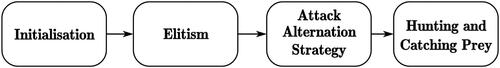
• Initialisation: During this step four matrices are initialised. The first one is SF_position matrix in which each element $S{F}_{i,j}$ denotes the j^th position of the i^th sailfish (predator). The second matrix is a coloumn matrix SF_fitness in which each element represents the best position of each sailfish obtained so far. The third matrix denotes the position each sardine(prey) and is represented as S_position. The fourth matrix represents a column matrix which holds the best position of each sardine obtained so far, and is represented as S_fitness.

• Elitism: The army of sail fish starts moving towards the target group and the best position of sail fish remains unchanged and this position is called elite. The elite sailfish position is stored in $X_{\mathit{\text{Elite}}\_\mathit{\text{SF}}}^i.$ The sardines gets injured by the unexpected tail movements of the sail fish and the position of the injured sardines are stored as $x_{\mathit{\text{Injured}}\_S}^i.$

• Attack alternation strategy: Sailfish never attack continuously or they never attack in group. They attack in a shrinking circle scenario. The attacking sailfish will now have a value given by 7 (Shadravan et al., 2019), where λ_i refers to a random number which varies according to the prey density. (7) $$x_{\mathit{\text{New}}\_\mathit{\text{SF}}}^i= x_{\mathit{\text{Elite}}\_\mathit{\text{SF}}}^i-{\lambda }_i\times (\mathit{\text{rand}}(0,1)\times \left[\frac{x_{\mathit{\text{Elite}}\_\mathit{\text{SF}}}^i+x_{\mathit{\text{Injured}}\_S}^i}{2}\right]-x_{\mathit{\text{old}}\_\mathit{\text{SF}}}^i)$$(7)

• Hunting and catching prey: The position of the injured sardines which are easy to capture are noted as 8, where the r refers to a random number between 0 and 1, AP refers to the attack power of the sailfish which keeps on decreasing as the iteration increases. (8) $$x_{\mathit{\text{new}}\_S}^i=r\times \left(x_{\mathit{\text{Elite}}\_\mathit{\text{SF}}}^i-x_{\mathit{\text{old}}\_S}^i+\mathit{\text{AP}}\right)$$(8)

3.3. Noise in SAR images

The noise in SAR is seen as a dark and white spots, similar to speckle, on the SAR data. This is created due to the multiple coherent reflections from the heterogeneous resolution cell (Le Toan, n.d.; Bhattacharya, n.d.). Hence the impact of noise and its characteristics vary according to the imaging platform’s technical specifications. It is impossible to find the characteristics of the noise influence in the images if the auxiliary data (technical specifications) is not available. Since the SAR image is obtained by sending the microwave range frequency signals through an antenna which keeps on moving (hence it provides a wide synthetic aperture) (Moreira et al., 2013), the scattered signals from the ground will have the fine details about the frequency, wavelength, incident angle and polarisation. These details may help in interpreting the scene under observation. But in real scenarios these auxiliary data may not be available with the SAR image. Under such conditions, it is necessary to analyse and interpret the image with its spatial components itself. Since Histogram is a pure representation of the frequency of the spatial coordinate values, in order to analyse the noise influence in the image separately, the histogram based estimation techniques can be adopted (Mu et al., 2019; Zhou et al., 2019).

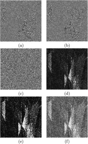
Since the noise in SAR is a deformation of the information, conventional linear filters fails to preserve the edge information. In most of the cases, an over smoothing occurs, and this degrades the performance of the algorithm. The log transformation is found to be useful in removing the multiplicative nature of the noise (Singh & Shree, 2016). SAR denoising is also found to be more accurate when the information is filtered in transform domain rather than spatial domain (Choi & Jeong, 2019). The proposed method adopts the advantages of optimized linear filters in transform domain. The SAR data taken in amplitude, intensity, phase and log intensity formats as shown in Figure 2 (Oliver & Quegan, 2004; Bhattacharya, n.d.).

Figure 2. Sample SAR image in different data formats- (a) Real in-phase, (b) Quadrature imaginary, (c) phase, (d) Amplitude, (e) Intensity, (f) Log intensity (Oliver & Quegan, 2004).

4. Proposed methodology

In the proposed method, denoising is preceded with a step which evaluates the noise distribution in real SAR images, and this ensures a better performance. In order to analyse the performance of the proposed method, the synthetic SAR images are corrupted with the noise whose model is determined in the previous step. For finding the performance of the system for practical conditions, full–reference and no–reference quality parameters are calculated, and the manual parameter optimization is performed.

4.1. Determining the noise model

The results of histogram-based studies state that the amplitude in the raw data is always found to be Rayleigh distributed and phase is always uniform distributed. In some applications, instead of the amplitude value, the intensity value is taken in to consideration and the intensity which is the squared amplitude is always found to be following a negative exponential distribution (Bhattacharya, n.d.). The SAR data intensity and amplitude are very much affected by the technical environment specifications under which the images are captured.

The survey on noise modelling by Gao and Gui in 2010 (Gao, 2010) states that the noise distribution in SAR images is very much depending on the nature of scene and those distributions can be tabulated as in Table 1. It is very clear from these observations that, since a real SAR is always heterogeneous in nature the noise would be either Rayleigh distributed or Gamma distributed. Hence most of the recent experiments on SAR data consider the noise to be G⁰ distributed, which is a special case of Gamma itself.

Table 1. Product distribution noise models (Gao, 2010).

Noise distributions	Category	Characteristics	Areas of applications
GC	Product Model	Model estimation and further interpretation is really complex	Used for images with extreme high resolution characteristics
RiIG		SAR noise model interpretation requires further investigation	Accurate for ultrasound images
U,W.		Not used	Used when the data is, Moderately Heterogeneous Multi look/Single look Intensity/Amplitude
G		Not used due to the difficulty in implementation	Used when the data is, Homogeneous/Heterogeneous/Extremely Heterogeneous Multi look/Single look Intensity/Amplitude
Gh		Special case of G distribution	Used when the data is extremely heterogeneous
Gamma		Amplitude data follows square root gamma distribution	Used when the data is, Homogeneous Multi look Intensity
Exponential		Used Widely	”
K		”	Used when the data is, Moderately Heterogeneous Multi look/Single look Intensity/Amplitude
G^0		”	Used when the data is, Homogeneous/Heterogeneous/Extremely Heterogeneous Multi look/Single look Intensity/Amplitude
β		Special case of G^0 distribution	Used when the data is, Homogeneous/Heterogeneous/Extremely Heterogeneous Single look Intensity

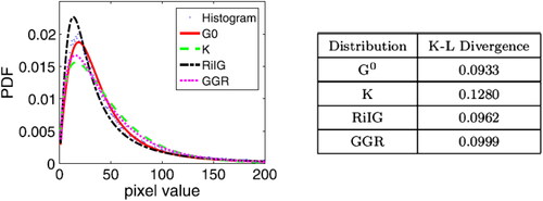
In a comparative experiment involving four different distributions (K, G₀, RiIG, and GGR models) on a real SAR image of an urban area, the study utilized the Kullback–Leibler divergence (KLD) to assess the fitting precision of normalized histograms and estimated density functions (Podest, 2017). The results demonstrated the superiority of the G₀ distribution, showcasing higher fitting precision compared to other models. Recent studies on statistical model comparisons have also confirmed the effectiveness of the G₀ distribution over other models across various resolutions, emphasizing its superior performance in SAR image analysis. The noise profile estimation plots and divergence values are given Figure 3 (Podest, 2017).

Figure 3. Noise profile estimation of SAR images (Podest, 2017).

According to G⁰ distribution the intensity of the back scattered signals follows inverse of the square root of Gamma distribution and the multiplicative speckle would follow square root of Gamma distribution, as shown in (9) (Mu et al., 2019). (9) $$P(f)=\frac{2L^L\Gamma (L-\alpha ){\gamma }^{-\alpha }{f}^{2L-1}}{\Gamma (L)\Gamma (-\alpha ){(\gamma +L{f}^2)}^{L-\alpha }},-\alpha ,\gamma ,L,f>0$$(9) where the term α represents the roughness of the area which backscatters the signals, γ represents the intensity of backscattered signals, L represents the equivalent number of looks and $\Gamma (.)$ denotes the Gamma function (Mu et al., 2019). The SAR images with G⁰ distribution shows an improvement in the image quality when the number of looks (L) parameter increases. Hence in this work we confine the noise to be G⁰ distributed.

4.2. Proposed SAR denoising algorithm

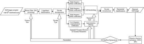
In this work a robust framework is designed and developed by using the advantages of Bitonic preprocessing filter and SailFish optimization in wavelet domain. After analysing the histogram of the input image, the noise model is determined, and then the output image is created with a series of processes which involves the following steps. First it is preprocessed with a Bitonic filter. As explained in Section 3.1, Bitonic filter consists of a combination of linear operators and non-linear morphological operators. Since there is no data-level-sensitive parameters the algorithm gets locally adapted to the noise levels and signal in an image, by preserving the minute details in an image without creating much artefactual noise (Goyal et al., 2022). Then the multiplicative impact of noise is reduced by logarithmic transformation. This log transformed data is wavelet decomposed to approximation and detail coefficients. Later, soft thresholding is done on the detail coefficients and the approximation coefficients are filtered using an optimized linear filter. Later, wavelet reconstruction is performed. Exponential transform on the reconstructed data retrieves the denoised image. All these processes and parameters are controlled and determined by the SailFish optimization technique (Shadravan et al., 2019). The selection of Sailfish optimization for this work was based on the previous literature and empirical study conducted. Sailfish optimization is suitable for real-time optimization applications due to its speed, adaptability to dynamic conditions, and efficient parallel processing capabilities. It can quickly find optimal or near-optimal solutions in rapidly changing environments, making it ideal for decision support systems that require quick adjustments. Its versatility in handling various types of optimization problems and its balance between exploration and exploitation ensure it continues to search for better solutions in real-time scenarios, enhancing its suitability for dynamic applications. The paramters optimized using this algorithm are provided in Table 2 and 3 for synthetic and real SAR data respectively.

Table 2. Optimal Parameters obtained for Sandia1 image using the proposed method.

Bitonic filter window size	Type of wavelet	Approximation filter	Threshold selection	Optimized SSIM
5	Daubechies 6	Imguided filter	Visushrink	.3426

Table 3. Optimal Parameters obtained for Quicklook1 image using the proposed method.

Bitonic filter window size	Type of wavelet	Approximation filter	NL means search window	NL Means similarity window	Threshold selection	Optimized EPI
3	Symlets 8	Non Local Means Filter	3	3	Visushrink	.97

For synthetic SAR data, the SailFish optimization takes SSIM (Wang et al., 2004) of the denoised image as the objective function. The capacity of EPI to simulate the statistical characteristics of SAR images is a primary factor in the selection of the software for genuine SAR data. Speckle noise in SAR images is well recognised for making them complicated and multiplicative. EPI is made to deal with this complexity well. It is ideally suited to capture the subtleties of actual SAR data since it takes into account the probability of witnessing a certain patch of data under a statistical model. Moreover, A broad variety of land cover types, objects, and topography are frequently included in real SAR data. EPI can take into consideration this heterogeneity because of its capacity to record the expected likelihood of patches. In the case of real SAR data the EPI is chosen (Sattar et al., 1997) as the objective function. Less than five iterations using SFO itself would yield the optimised parameters for the algorithm. There are six parameters determined by the optimization. The first parameter decides the Bitonic filter window size (Goyal et al., 2022), second one determines the wavelet type used for decomposition and reconstruction (Choi & Jeong, 2019). The third parameter is for threshold value selection for wavelet decomposed detail coefficients (if the value is one, visushrink is used and if it is two wthresh matlab tool is used, and if it is three then bayes shrink is used) (Rai et al., 2012). The fourth one selects the approximation filter (ie; if the parameter is one, then guided filter (He et al., 2012) is used and if it is two then Non local means filter (NL means) is used), the fifth and sixth parameters determines the search and similarity window of non local means filter, respectively (Buades et al., 2005). The block diagram of the proposed method is shown in Figure 4.

Figure 4. Block Diagram of the Proposed SAR Denoising Algorithm.

5. Experimental setup

SAR images are corrupted in nature (corrupted by origin) ie; their purest form is not available. In order to analyse the performance of the denoising algorithms the purest form of the image is necessary, hence the experiments must be carried on some synthetic SAR images which possess the characteristics of the real SAR images. These synthetic SAR images when corrupted with the G⁰ distributed noise will be exact look alike of real SAR data, but their pure and corrupted versions will be available. In this work the performance of the proposed algorithm is tested on nine synthetic SAR images such as [Sandia1, Sandia2, Sandia3] from Sandia National Laboratories of U.S. Government (Sandia National Laboratories of U.S. Government, n.d.), [JPL1, JPL2, JPL3] from NASAPHOTOJOURNAL – jet population Laboratories (NASA PHOTOJOURNAL – jet population Laboratories, n.d.), and [Airbus1, Airbus2, Airbus3] from Satellite Imagery – Airbus Defense and Space (Satellite Imagery – Airbus Defense and Space, n.d.). The proposed filter’s performance is measured with three real SAR images [quicklook1, quicklook2, quicklook3] from Sentinel Copernicus data hub (The Copernicus Open Access Hub, n.d.).

The performance of the proposed method is compared with the performance of 4 state-of-the-art denoising methods. Method 1 (FOTV) represents the speckle reducing anisotropic diffusion filter from despeckle filtering software toolbox designed for ultrasound imaging of the common carotid artery (Wang et al., 2022). Method 2 (BMDL) inlcudes an image despeckling method based on block matching and CNN architecture (Wang et al., 2022). Method 3 (EFO-DTCWT), includes despeckling SAR images using DTCWT based local adaptive thresholding enhanced by fruit fly optimization (Kumar et al., 2021). Finally, Method 4 (NLJSM), represents guided patchwise nonlocal SAR despeckling (Liang et al., 2022). All experiments are conducted in MATLAB version R2017b on Intel(R), Core(TM), i3-7020U, CPU 2.30 GHz, 4 GB RAM and 64-bit operating system. The same system configuration is used to opinion the execution time of the proposed algorithm and the existing techniques.

The algorithm proposed here is tested in two steps. As the first step the G⁰ distributed noise is added to the synthetic SAR images and after denoising the quality parameters are calculated by taking the pure image as reference. In the second step the noisy real SAR data is taken and the de-noised version undergoes the no-reference quality evaluation (Anandhi & Valli, 2018). Full reference quality evaluation metrics requires two images, an image which needs to be analysed and a reference image. In this work the de-noised synthetic SAR images are compared with the pure versions of those images. This analysis is done by calculating the following parameters (Anandhi & Valli, 2018).

• Root Mean Square Error – RMSE: The RMSE value provides an indication about the change happened per pixel due to the processing. The lower the value this parameter the higher will be the quality of the image (Huynh-Thu & Ghanbari, 2008).

• Peak Signal to Noise Ratio – PSNR: The PSNR measures the peak signal to noise ratio between 2 images in decibels (Huynh-Thu & Ghanbari, 2008).

• Structural Similarity Index Measures – SSIM: Unlike RMSE and PSNR which calculates the mean errors, the SSIM value provides more detailed comparison based on the visual structures and perception in the reference image and the original image. Higher the value of SSIM better would be the noise quality and the value ranges from –1 to 1 (Wang et al., 2004).

• Universal Image Quality Index – UIQI: This provides an indication about the linear correlation, contrast and luminance. This value ranges from 0 to 1 and the higher value denotes a better image (Anandhi & Valli, 2018).

Full reference based quality evaluation is only possible when the pure reference image is available. When real SAR data is taken in to consideration the image which is obtained from the SAR imaging process itself is corrupted. Hence more sophisticated evaluation metrics which could analyse the image under test without the reference image needs to be used (Anandhi & Valli, 2018). Such evaluation metrics used in our study are mentioned below;

• Noise Mean Variance – NMV: The noise content in the de-noised image can be calculated by the parameter called as Noise Mean Variance (NMV). The lower value of this parameter indicates a better image quality (Anandhi & Valli, 2018).

• Noise Variance – NV: Similarly the noise content in the de-noised image can also be calculated by the parameter called as Noise variance (NV). The image quality increases for a lower noise variance value (Anandhi & Valli, 2018).

• Mean Square Difference – MSD: The mean difference of pixel intensities between the real SAR image and the de-noised image is indicated by the Mean Square Difference value. The increment in the value of MSD indicates a better denoising process (Anandhi & Valli, 2018).

• Equivalent Number of Looks – ENL: The smoothing effect of the denoising algorithm is well represented by the parameter called as Equivalent Number of Looks (ENL). A higher value indicates a better performance (Anandhi & Valli, 2018).

• Noise Level Estimate – NLE: NLE computes the noise level in an image by a patch based noise level estimation algorithm (Liu et al., 2013). The noise level in patches are computed with the help of principle component analysis (PCA). If the patches are weak due to the noise content then selection of patches is done based on the gradients of the patches and their statistics. Then the noise level is estimated using PCA.

6. Results and discussion

The experiments are executed in four phases. During the first phase the noise distribution in real SAR data which is taken for experiment is analysed by performing a histogram based analysis. The second phase implements the proposed algorithm on the synthetic and real SAR dataset. The third phase compares the performance of the proposed algorithm on synthetic SAR data from different databases with the existing denoising methods. Then during the fourth phase the real SAR data images are taken and the performance of the proposed algorithm on this data is verified by taking the no-reference quality parameters in to consideration. Figures 5–15 and Tables 4–7 depicts the qualitative and quantitative comparison of synthetic and SAR images.

Figure 5. Sandia2 image corrupted with G⁰ noise, after denoising with the proposed algorithm and other conventional algorithms.

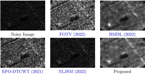
Figure 6. Sandia3 image corrupted with G⁰ noise, after denoising with the proposed algorithm and other conventional algorithms.

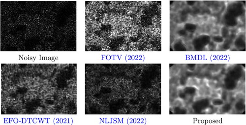
Figure 7. Airbus1 image corrupted with G⁰ noise, after denoising with the proposed algorithm and other conventional algorithms.

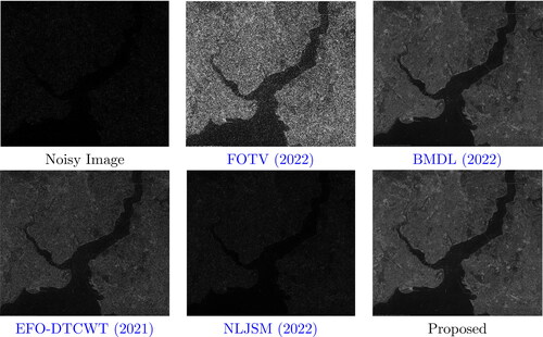
Figure 8. Airbus2 image corrupted with G⁰ noise, after denoising with the proposed algorithm and other conventional algorithms.

Figure 9. Airbus3 image corrupted with G⁰ noise, after denoising with the proposed algorithm and other conventional algorithms.

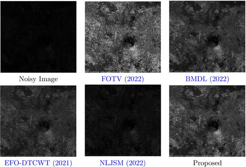
Figure 10. JPL1 image corrupted with G⁰ noise, after denoising with the proposed algorithm and other conventional algorithms.

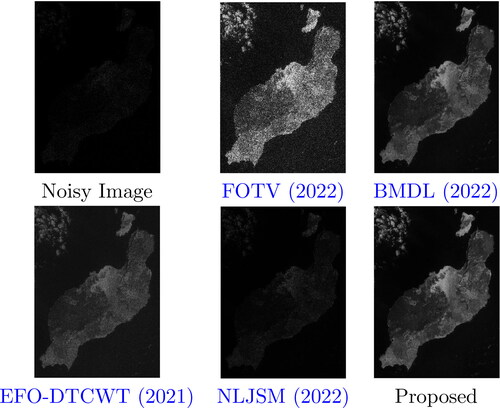
Figure 11. JPL2 image corrupted with G⁰ noise, after denoising with the proposed algorithm and other conventional algorithms.

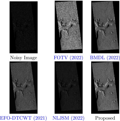
Figure 12. JPL3 image corrupted with G⁰ noise, after denoising with the proposed algorithm and other conventional algorithms.

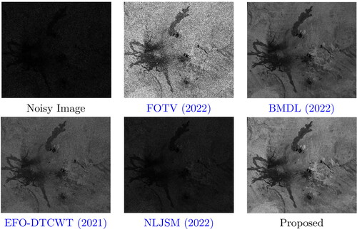
Figure 13. Real SAR image quicklook1, after denoising with the proposed algorithm and other conventional algorithms.

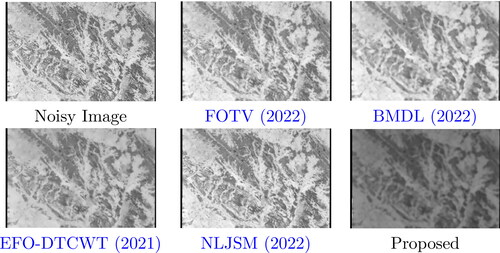
Figure 14. Real SAR image quicklook2, after denoising with the proposed algorithm and other conventional algorithms.

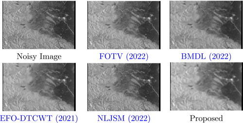
Figure 15. Real SAR image quicklook3, after denoising with the proposed algorithm and other conventional algorithms.

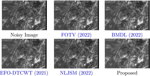
Table 4. Performance of different denoising algorithms on Sandia1, Sandia2 and Sandia3 images.

Method Parameters	RMSE			PSNR			SSIM			UIQI
	Sandia1	Sandia2	Sandia3	Sandia1	Sandia2	Sandia3	Sandia1	Sandia2	Sandia3	Sandia1	Sandia2	Sandia3
Noisy	111.03076	94.02	101.9	7.25	8.68	7.99	0.0563	0.1073	0.1144	0.0594	0.1165	0.1301
FOTV (2022)	64.3937	59.3554	59.4422	11.9539	12.6616	12.6489	0.097	0.1561	0.1743	0.1032	0.17	0.2003
BMDL (2022)	23.2791	24.0534	23.2606	20.7915	20.5073	20.7984	0.3171	0.3773	0.5013	0.2214	0.285	0.4562
EFO-DTCWT (2021)	39.5608	34.7471	36.5611	16.1855	17.3124	14.8267	0.2079	0.317	0.3793	0.1797	0.3061	0.3819
NLJSM (2022)	47.0291	42.0492	46.2599	14.6835	15.6557	16.8704	0.1719	0.2784	0.333	0.1628	0.2759	0.3378
Proposed	22.195	24.0225	22.6103	21.2057	20.5184	21.0447	0.3426	0.3674	0.5174	0.2361	0.264	0.4665

Table 5. Performance of different denoising algorithms on Airbus1, Airbus2 and Airbus3 images.

Method Parameters	RMSE			PSNR			SSIM			UIQI
	Airbus1	Airbus2	Airbus3	Airbus1	Airbus2	Airbus3	Airbus1	Airbus2	Airbus3	Airbus1	Airbus2	Airbus3
Noisy	105.36	99.81	93.71	7.715	8.17	8.71	0.8036	0.8318	0.8532	0.18592	0.1742	0.0843
FOTV (2022)	60.3193	59.5505	55.6819	12.5217	12.6331	13.2165	0.828	0.8492	0.867	0.259	0.2402	0.1228
BMDL (2022)	38.4785	31.7811	21.1527	16.4264	18.0874	21.6235	0.8379	0.8666	0.8898	0.1826	0.2311	0.2527
EFO-DTCWT (2021)	44.9121	40.699	34.0251	15.0835	15.9391	17.4948	0.7972	0.8161	0.8388	0.3168	0.3102	0.2156
NLJSM (2022)	50.9215	46.7274	42.8417	13.9928	14.7394	15.4935	0.8318	0.8568	0.874	0.3267	0.3338	0.2124
Proposed	38.4301	32.0819	20.7244	16.4374	18.0056	21.8012	0.8467	0.8715	0.8987	0.1657	0.1708	0.2131

Table 6. Performance of different denoising algorithms on JPL1, JPL2 and JPL3 images.

Method Parameters	RMSE			PSNR			SSIM			UIQI
	JPL1	JPL2	JPL3	JPL1	JPL2	JPL3	JPL1	JPL2	JPL3	JPL1	JPL2	JPL3
Noisy	71.87	104.606	161.23	11.03	7.78	4.05	0.897	0.53192	0.6541	0.034	0.3159	0.01646
FOTV (2022)	40.2696	56.1001	73.5393	16.0313	13.1515	10.8004	0.9043	0.5934	0.7124	0.053	0.325	0.0332
BMDL (2022)	15.0239	16.3848	24.6506	24.5952	23.842	20.2942	0.9217	0.6389	0.7064	0.1505	0.405	0.1792
EFO-DTCWT (2021)	25.631	35.1726	55.8566	19.9555	17.2067	13.1893	0.8942	0.5728	0.6824	0.1064	0.0611	0.0858
NLJSM (2022)	37.2389	45.6061	69.2693	16.7109	14.9503	11.32	0.91	0.5686	0.6834	0.0952	0.3405	0.0698
Proposed	14.6333	14.8241	21.2322	24.824	24.7114	21.5909	0.9315	0.6526	0.739	0.1309	0.1178	0.1884

Table 7. Performance of different denoising algorithms on real SAR images.

Method Parameters	ENL			MSD			NV			NMV			NLE
	QL1	QL2	QL3	QL1	QL2	QL3	QL1	QL2	QL3	QL1	QL2	QL3	QL1	QL2	QL3
Noisy	14.5705	6.2732	6.8899	Not Applicable			810.3639	1006.5	1471.7	108.6618	79.4619	100.6971	1.61	2.3047	2.0036
FOTV (2022)	17.7197	7.6607	7.647	42.2046	56.6594	50.4748	666.3332	823.9769	1325.9	108.661	79.4497	100.6945	1.0223	1.4831	1.2937
BMDL (2022)	18.4665	8.1187	7.8329	109.7061	159.9889	132.0282	639.1496	772.9927	1292.8	108.6409	79.2195	100.6307	0.6002	0.659	0.4839
EFO-DTCWT (2021)	19.1598	8.3663	7.9993	99.1277	111.3995	131.656	569.2902	704.2643	1168.7	104.439	76.7599	96.6875	0.0074	0.0126	0.0068
NLJSM (2022)	16.3844	7.143	7.4459	32.9471	43.5938	46.1321	721.0162	881.1011	1360.3	108.6897	79.3328	100.6421	0.1351	1.11	0.2103
Proposed	19.5851	8.9936	8.0435	173.8001	225	193.4679	556.0789	650.1034	1160.5	104.3592	76.4642	96.614	0.0013	0.0013	0.00074759

6.1. Phase 1: Noise estimation in real SAR data

Since the histogram plots of an image is the graphical representation of the distribution of pixel intensities in an image, the noise distribution in SAR data can be understood from their histogram plots. The real SAR data used in this paper are quicklook1, quicklook2, quicklook3 from Sentinel Copernicus data hub. The quicklook1 image is homogeneous in nature, quicklook2 is moderately heterogeneous and quicklook3 is extremely heterogeneous. The real SAR images with different levels of heterogeneity and their respective histogram plots are shown in Figure 16.

Figure 16. Real SAR images obtained from sentinel data hub and their corresponding histogram plots.

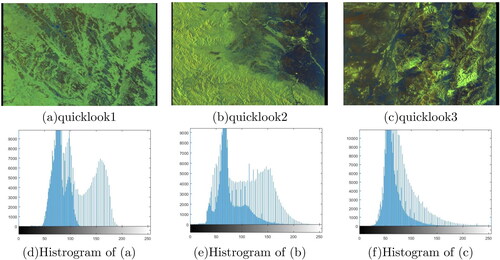
The histogram plots shows that the observations made by Gao and Gui (Gao, 2010), are satisfying with the results obtained. For homogeneous image the noise distribution will be similar to that of Rayleigh distribution and as the heterogeneity increases the noise starts getting distributed in Gamma and special Gamma formats i.e.; G⁰ distribution.

6.2. Phase 2: Proposed denoising

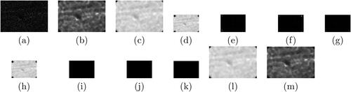
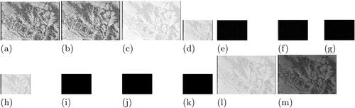
The proposed method is first tested on synthetic SAR data for a better performance analysis. Since the synthetic SAR is not noisy, the estimated G⁰ distributed noise is multiplied with the original pixels in the image to get the noisy version Figure 17(a). During the $1^{\mathit{\text{st}}}$ iteration in SFO it is preprocessed with a Bitonic filter to remove the impulsive noises. The log transformation is applied and then the DWT decomposes the image to approximation and detail coefficients. Filtering and thresholding are done on approximation and detail coefficients respectively. Then wavelet reconstruction followed with an exponential transform yields an intermediate output image. This image is processed and the objective function SSIM is calculated. SFO iterates, finds the best parameters (Bitonic filter window size, wavelet type, approximation filter, approximation filter parameters and the type of detail coefficient thresholding) and then perform denoising on the noisy image with the proposed method and its optimized parameters. The intermediate outputs of the proposed denoising method on Sandia1 image after finding the optimised parameters are given in Figure 17. The optimised parameters obtained for Sandia1 image are noted in Table 2.

Figure 17. The intermediate outputs after denoising Sandia1 image (synthetic SAR) corrupted with G⁰ noise using the proposed method (a) Noisy image, (b) Preprocessed image, (c) Log transformed image, (d) Approximation coefficients after DWT, (e)–(g) Detail horizontal, vertical, and diagonal components after DWT, (h) Filtered approximation component, (i)–(k) Thresholded detail components, (l) DWT reconstructed image, (m) Exponential transformed image.

The real SAR image itself is noisy hence for the performance analysis the no reference quality parameters explained in $5^{\mathit{\text{th}}}$ section are used. The procedure for denoising a real SAR image is similar to that of the synthetic SAR images. The difference only comes in the calculation of the objective function for the SailFish optimization. Real SAR images are optimized by considering a better value for the EPI. The intermediate outputs of the proposed denoising method on Sandia1 image after finding the optimised parameters are given in Figure 18. The optimised parameters obtained for Quicklook1 image are noted in Table 3.

Figure 18. The intermediate outputs after denoising Quicklook1 image (real SAR) corrupted with G⁰ noise using the proposed method [(a) Noisy image, (b) Preprocessed image, (c) Log transformed image, (d) Approximation coefficients after DWT, (e)–(g) Detail horizontal, vertical, and diagonal components after DWT, (h) Filtered approximation component, (i)–(k) Thresholded detail components, (l) DWT reconstructed image, (m) Exponential transformed image.

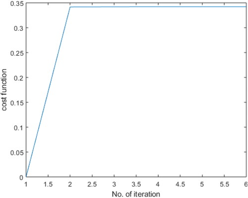
All the parameters used in this method are optimized using the SailFish optimization. The objective function attains the best value even after the first two iterations. The graph showing the value of the objective function during optimization is the same for both real and synthetic SAR data, graph plots are shown in Figure 19.

Figure 19. Parameter optimization graph of proposed method.

6.3. Phase 3: Performance Comparison – Synthetic SAR images

Nine sample images from three different datasets are presented for the performance analysis. The corrupted images are passed through five different filters including the proposed filter and the values obtained for different full reference quality parameters are noted in tabular format.

Sandia1 and Sandia3 images are showing a better performance for the proposed filter design for all the parameters when compared with all other filters. The de-noised images after different methods are shown Figure 6 and Figure 20 respectively. Whereas Sandia2 shows a better RMSE and PSNR values for the proposed method but the SSIM and UIQI are little less when compared with method 1. But this performance can not be generalised because sandia image are of low resolution whereas the real SAR data is always high resolution. The results of Sandia2 is shown in Figure 5. The corresponding quality parameters for each of those images are noted in Table 4.

Figure 20. Sandia1 image corrupted with G⁰ noise, after denoising with the proposed algorithm and other conventional algorithms.

Since Sandia images are of poor resolution, for a better understanding regarding the performance images from other datasets are also taken in to consideration. Airbus1 and Airbus3 are showing better RMSE, PSNR and SSIM values for the proposed method. Whereas for Airbus2 the RMSE and PSNR are better for method 1 and SSIM is better for proposed method. Since SSIM is a better indication regarding the edge preservation, we can say that the proposed method is better for all the three images. The de-noised outputs of airbus1, airbus2 and airbus3 are shown in Figure 7, Figure 8 and Figure 9 respectively. The quality parameters are noted in Table 5.

The JPL1, JPL2 and JPL3 images are used for the performance analysis. These images with a good resolution are showing a better performance for the proposed filter design. The RMSE, PSNR and SSIM values are better when compared with all other filters. Sandia images are web images which were compressed to a lower resolution (size in the order of kilobytes) and a real SAR image could never be of this much poor resolution. This indicates that a SAR image which is of proper resolution is expected to perform better for the proposed filter design. The experimental results for JPL1, JPL2, and JPL3 are shown in Figure 10, Figure 11 and Figure 12 respectively and the quality parameters are noted in Table 6.

The sandia image, Airbus image and JPL image are all synthetic SAR images but they differ from each other in their size. The resolution of Airbus image and JPL image are far better than that of Sandia images. The Sandia images are web images which are already compressed but possess the features of SAR images. A real SAR image is always of higher resolution. The Airbus and JPL are showing better performance for the proposed filter hence a real SAR image of better resolution should work well the proposed filter design.

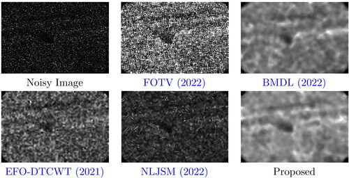
6.4. Phase 4: Performance comparison – Real SAR images

The performance of the proposed system is better with the synthetic SAR images which have good resolution. Now during this phase the filter is tested on, the real SAR images obtained from Copernicus sentinel data hub. SAR images are captured through the techniques of coherent imaging. They are corrupted with the similar kind of multiplicative speckle as well. Three real SAR images are considered here. Since their purest form is not available the quality of the de-noised image is calculated with the help of no-reference quality metrics. The experiment shows that for all the four images, the proposed filter is showing better quality parameter values. The output images of quicklook1, quicklook2 and quicklook3 after different denoising techniques are shown in Figure 13, Figure 14 and Figure 15 respectively. The respective no-reference quality parameters are also tabulated in Table 7. The performance of the proposed filter on real SAR data indicates that the no reference quality parameters are far better for an image denoised with the proposed filter when compared with the noisy one and the existing algorithms. All the four real images are showing better parameters for the proposed filter, but when all the three real SAR images are compared, the extremely heterogeneous image quicklook3 is showing a remarkable increment in all the parameters when compared with all other four existing algorithms.

7. Conclusion

In conclusion, the developed framework for removing G0 distributed noise from Synthetic Aperture Radar (SAR) images represents a significant advancement in enhancing image quality and preserving valuable information in SAR data analysis. The proposed algorithm involves pre-processing with an optimized Bitonic filter, log transformation to convert multiplicative noise to additive, wavelet decomposition, optimized linear filtering of approximation coefficients, and soft thresholding of detail coefficients. This method outperforms conventional denoising techniques, showing improved quality parameters for both synthetic and real SAR images. Quantitative and qualitative comparison of the proposed method is done with the state-of-the-art algorithms. The proposed design is showing better full reference quality parameters for synthetic SAR images from three different datasets and better no-reference quality parameters for real SAR images. The algorithm ensures better edge preservation and enhances image quality through quantitative metrics like structural similarity index and noise level estimation.

The time requirement and complexity in the optimisation used in this proposed algorithm is a scope for future research. Quantum-inspired algorithms like QAB algorithm and DeQuIP algorithm have demonstrated their potential in some applications. Nevertheless, there is insufficient empirical data to support their superiority over classical denoising techniques for SAR images. The future scope of this study includes exploring them for inclusion for SAR image analysis studies as well.

Author contributions

Formal analysis, Ragesh M and Vinayababu M; Investigation, Ragesh M and Vinayababu M; Methodology, Ragesh M; Resources, Vinayababu M; Software, Vinayababu M; Supervision, Shilpa Suresh; Validation, Shilpa Suresh; Writing – original draft, Vinayababu M; Writing – review and editing, Ragesh M and Shilpa Suresh.

Acknowledgements

The authors wish to express their appreciation to the anonymous reviewers for their thorough review and helpful suggestions.

Disclosure statement

No potential conflict of interest was reported by the author(s).

Data availability statement

The data used in this study will be made available from the corresponding author on a reasonable request.

Additional information

Notes on contributors

Rajan M. Ragesh

Ragesh Rajan M. holds a bachelor’s degree in Electronics and Communication Engineering and master’s degree in Communication Engineering and Signal Processing from Govt. Engineering College Thrissur, affiliated to University of Calicut, Kerala. He completed his Ph.D. in Signal Processing and Machine Learning from the National Institute of Technology Karnataka, Surathkal. Since 2022, he is serving as an Assistant Professor in the Department of Electronics and Communication Engineering at Amrita Vishwa Vidyapeetham, Amritapuri, Kerala. He has served as an Assistant Professor in the Department of Electronics and Communication Engineering at MES College of Engineering, Kuttippuram, Kerala. He has been a teacher for more than 12 years and has published papers in prestigious journals by IEEE, Elsevier and Taylor and Francis and has authored and co-authored papers in prestigious conferences such as ICASSP and INTERSPEECH. His research interests include Machine Learning, Speech Signal Processing, Music Signal Processing and Image Processing.

M. Vinayababu

Vinayababu M. completed her bachelor’s degree in Electronics and Communication Engineering and a master’s in Communication Systems and Signal Processing from Kerala Technological University, India. Her research interests are in the fields of Image Processing, Optimization Algorithms and Artificial Intelligence, and Machine Learning.

Suresh Shilpa

Shilpa Suresh holds a bachelor’s degree in Electronics and Communication Engineering from Calicut University, a master’s in Communication Systems from Hindustan University, and a Ph.D. in Satellite Image Processing from the National Institute of Technology Karnataka. Since 2012, she has been dedicated to teaching and research, contributing to numerous publications in esteemed journals such as IEEE, Elsevier, Springer, Taylor and Francis etc. Her academic prowess is complemented by certifications from various international universities through online courses and contributes as a reviewer for prestigious journals and conferences. As a Senior member of IEEE, she currently serves as Joint Secretary for the IEEE Geoscience and Remote Sensing Society, Bangalore Section. Additionally, she is engaged in professional societies like ISTE and IAENG. Her research interests span Image Processing, Optimization Algorithms, Artificial Intelligence, Machine Learning and Robotics. Notably, she secured the university first rank for her master’s degree and received the Best Ph.D. Thesis Award at the MIND 2019 Ph.D. Symposium hosted by the National Institute of Technology Kurukshethra.

References

- Amirmazlaghani, M., & Amindavar, H. (2009). A novel statistical approach for speckle filtering of SAR images. In 2009 IEEE 13th Digital Signal Processing Workshop and 5th IEEE Signal Processing Education Workshop. IEEE. https://doi.org/10.1109/DSP.2009.4785967
- Anandhi, D., & Valli, S. (2018). An enhanced approach to Despeckle SAR images. Radioengineering, 27(3), 864–875. https://doi.org/10.13164/re.2018.0864
- Bhattacharya, A. (n.d.). Speckle filtering or speckle statistics, Retrieved from http://www.csre.iitb.ac.in/avikb/GNR647/Lec11Speckle.pdf.
- Buades, Antoni, Bartomeu, Coll, & Morel, J.-M. (2005). A non-local algorithm for image denoising Computer Vision and Pattern Recognition. In 2005 IEEE computer society conference on computer vision and pattern recognition (CVPR'05), vol. 2, pp. 60–65.
- Chen, W. F., Liu, A. L., Xia, J. J., Duan, C. L., Yang, S. S., & Hu, W. C. (2014). Study on synthetic aperture radar image denoising algorithm. Applied Mechanics and Materials, 599–601, 1734–1737. https://doi.org/10.4028/www.scientific.net/AMM.599-601.1734
- Chitroub, S., Houacine, A., & Sansal, B. (2002). Statistical characterisation and modeling of SAR images. Signal Processing, 82(1), 69–92. https://doi.org/10.1016/S0165-1684(01)00158-X
- Choi, H., & Jeong, J. (2019). Speckle noise reduction technique for SAR images using statistical characteristics of speckle noise and discrete wavelet transform. Remote Sensing, 11(10), 1184. https://doi.org/10.3390/rs11101184
- Choi, H., Yu, S., & Jeong, J. (2019). Speckle noise removal technique in SAR images using SRAD and weighted least squares filter. In 2019 IEEE 28th International Symposium on Industrial Electronics (ISIE). IEEE. https://doi.org/10.1109/ISIE.2019.8781457
- Delignon, Y., Garello, R., & Hillion, A. (1997). Statistical modeling of ocean SAR images. IEE Proceedings-Radar, Sonar and Navigation, 144(6), 348–354.
- Du, Y., Zhong, R., Li, Q., & Zhang, F. (2022). TransUNet++SAR: Change detection with deep learning about architectural ensemble in SAR images. Remote Sensing, 15(1), 6. https://doi.org/10.3390/rs15010006
- Frery, A. C., Correa, A., Renno, C. D., Corina da da, C. F., Jacobo-Berlles, J., Vasconcellos, K. L., Mejail, M., & Sant'anna, S. J. (1999a). Models for synthetic aperture radar image analysis. Resenhas Do Instituto de Matemática e Estatística da Universidade de São Paulo, 4(1), 45–77.
- Frery, A. C., Freitas, C., Sant'anna, S. J., & Rennó, C. D. (1999b). Statistical properties of SAR data and their consequences. United Nations Programme on Space Applications, 10, 53.
- Frost, V. S., Stiles, J. A., Shanmugan, K. S., & Holtzman, J. C. (1982). A model for radar images and its application to adaptive digital filtering of multiplicative noise. IEEE Transactions on Pattern Analysis and Machine Intelligence, 4(2), 157–166. https://doi.org/10.1109/tpami.1982.4767223
- Gao, G. (2010). Statistical modeling of SAR images: A survey. Sensors, 10(1), 775–795. https://doi.org/10.3390/s100100775
- Gayathri, R., & Sabeenian, R. S. (2012). A Survey on Image Denoising Algorithms (IDA). International Journal of Advanced Research in Electrical, Electronics and Instrumentation Engineering, 1(5), 456–462.
- Goyal, B., Gupta, A., Dogra, A., & Koundal, D. (2022). An adaptive bitonic filtering based edge fusion algorithm for Gaussian denoising. International Journal of Cognitive Computing in Engineering, 3, 90–97. https://doi.org/10.1016/j.ijcce.2022.03.001
- Halidou, A., Mohamadou, Y., Ari, A. A. A., & Zacko, E. J. G. (2023). Review of wavelet denoising algorithms. Multimedia Tools and Applications, 82(27), 41539–41569. https://doi.org/10.1007/s11042-023-15127-0
- Hao, Y., & Xu, J. (2014). An effective dual method for multiplicative noise removal. Journal of Visual Communication and Image Representation, 25(2), 306–312. https://doi.org/10.1016/j.jvcir.2013.11.004
- He, K., Sun, J., & Tang, X. (2012). Guided image filtering. IEEE Transactions on Pattern Analysis and Machine Intelligence, 35(6), 1397–1409. https://doi.org/10.1109/TPAMI.2012.213
- Henri, M. (2008). Processing of synthetic aperture radar images. Willey.
- Huang, Y.-M., Ng, M. K., & Wen, Y.-W. (2009). A new total variation method for multiplicative noise removal. SIAM Journal on Imaging Sciences, 2(1), 20–40. https://doi.org/10.1137/080712593
- Huynh-Thu, Q., & Ghanbari, M. (2008). Scope of validity of PSNR in image/video quality assessment. Electronics Letters, 44(13), 800–801. https://doi.org/10.1049/el:20080522
- Jebur, R., Sabah., & C. S., Der. (2023). Dalal Adulmohsin Hammood, and Leong Yeng Weng. Image denoising techniques: An overview. In AIP Conference Proceedings, vol. 2804, no. 1. AIP Publishing.
- Kumar, B., Kumar Ranjan, R., & Husain, A. (2021). A multi-objective enhanced fruit fly optimization (MO-EFOA) framework for despeckling SAR images using DTCWT based local adaptive thresholding. International Journal of Remote Sensing, 42(14), 5493–5514. https://doi.org/10.1080/01431161.2021.1921875
- Lattari, F., Gonzalez Leon, B., Asaro, F., Rucci, A., Prati, C., & Matteucci, M. (2019). Deep learning for SAR image despeckling. Remote Sensing, 11(13), 1532. https://doi.org/10.3390/rs11131532
- Le Toan, T. (n.d.). Advanced training course on land remote sensing, Retrieved from https://earth.esa.int/landtraining07/D1LA1-LeToan.pdf.
- Lee, J.-S. (1981). Speckle analysis and smoothing of synthetic aperture radar images. Computer Graphics and Image Processing, 17(1), 24–32. https://doi.org/10.1016/S0146-664X(81)80005-6
- Liang, D., Jiang, M., & Ding, J. (2022). Fast patchwise nonlocal SAR image despeckling using joint intensity and structure measures. IEEE Journal of Selected Topics in Applied Earth Observations and Remote Sensing, 15, 6283–6293. https://doi.org/10.1109/JSTARS.2022.3195093
- Liu, S., Pu, N., Cao, J., & Zhang, K. (2022). Synthetic Aperture radar image despeckling based on multi-weighted sparse coding. Entropy, 24(1), 96. https://doi.org/10.3390/e24010096
- Liu, X., Tanaka, M., & Okutomi, M. (2013). Single-image noise level estimation for blind denoising. IEEE Transactions on Image Processing, 22(12), 5226–5237. https://doi.org/10.1109/TIP.2013.2283400
- Lopez-Martinez, C. (2013). Speckle noise characterization and filtering in polarimetric SAR data, Eur. Space Agency, Paris, France. Retrieved fom https://earth.esa.int/documents/10174/669756/Speckle_Noise_Characterisation.pdf.
- Ma, X., Hu, H., & Wu, P. (2022). A no-reference edge-preservation assessment index for SAR image filters under a bayesian framework based on the ratio gradient. Remote Sensing, 14(4), 856. https://doi.org/10.3390/rs14040856
- Majee, S., Ray, R. K., & Majee, A. K. (2022). A new non-linear hyperbolic-parabolic coupled PDE model for image despeckling. In IEEE Transactions on Image Processing, 31, 1963–1977. https://doi.org/10.1109/TIP.2022.3149230
- Martinez-Espla, J. J., Martinez-Marin, T., & Lopez-Sanchez, J. M. (2009). A particle filter approach for InSAR phase filtering and unwrapping. IEEE Transactions on Geoscience and Remote Sensing, 47(4), 1197–1211. https://doi.org/10.1109/TGRS.2008.2008095
- Moreira, A., Prats-Iraola, P., Younis, M., Krieger, G., Hajnsek, I., & Papathanassiou, K. P. (2013). A tutorial on synthetic aperture radar. IEEE Geoscience and Remote Sensing Magazine, 1(1), 6–43. https://doi.org/10.1109/MGRS.2013.2248301
- Mu, Y., Huang, B., Pan, Z., Yang, H., Hou, G., & Duan, J. (2019). An enhanced high-order variational model based on speckle noise removal with G0 distribution. IEEE Access, 7, 104365–104379. https://doi.org/10.1109/ACCESS.2019.2931581
- Mullissa, A. G., Marcos, D., Tuia, D., Herold, M., & Reiche, J. (2022). deSpeckNet: Generalizing deep learning-based SAR image despeckling. In IEEE Transactions on Geoscience and Remote Sensing, 60, 1–15. https://doi.org/10.1109/TGRS.2020.3042694
- NASA PHOTOJOURNAL – jet population Laboratories. (n.d.). Retrieved from https://photojournal.jpl.nasa.gov/.
- Oliver, C., & Quegan, S. (2004). Understanding synthetic aperture radar images. SciTech Publishing.
- Painam, R. K., & Suchetha, M. (2023). Despeckling of SAR images using BEMD-based adaptive frost filter. Journal of the Indian Society of Remote Sensing, 51(9), 1879–1890. https://doi.org/10.1007/s12524-022-01495-x
- Parhad, S. V., Warhade, K. K., & Shitole, S. S. (2023). Speckle noise reduction in sar images using improved filtering and supervised classification. Multimedia Tools and Applications, 83(18), 54615–54636. https://doi.org/10.1007/s11042-023-17648-0
- Podest, E. (2017). Basics of synthetic aperture radar.
- Rafati, M., Kalantari, N., Azadbakht, J., Nickfarjam, A. M., & Hosseini, F. (2023). Performance evaluation of fuzzy genetic, fuzzy particle swarm and similar insects’ optimization algorithms on denoising problem based on novel combined filter for digital X-ray and CT images in Pelvic Region. Multimedia Tools and Applications, 2023, 1–49. https://doi.org/10.1007/s11042-023-15341-w
- Rai, R. K., Asnani, J., & Sontakke, T. R. (2012). Review of shrinkage techniques for image denoising. International Journal of Computer Applications, 42(19), 13–16. https://doi.org/10.5120/5799-8009
- Raju, K. M. S., Nasir, M. S., & Meera Devi, T. (2013). Filtering techniques to reduce speckle noise and image quality enhancement methods on satellite images. IOSR Journal of Computer Engineering, 15(4), 10–15. https://doi.org/10.9790/0661-1541015
- Rathore, M. S. (2014). Statistical analysis of Synthetic Aperture Radar (SAR) image speckle Diss.
- Ray, A., & Kartikeyan, B. (2015). Denoising techniques for synthetic aperture radar data – A review. International Journal of Computer Engineering and Technology, 6(9), 1–11.
- Roy, N., & Jain, V. (2015). Additive and multiplicative noise removal by using gradient histogram preservations approach. International Journal of Computer Applications, 130(2), 11–16. https://doi.org/10.5120/ijca2015906876
- Sandia National Laboratories of U.S Government. (n.d.). Retrieved from https://www.sandia.gov/.
- Satellite Imagery – Airbus Defense and Space. (n.d.). Retrieved from https://www.airbus.com/space/earth-observation.html.
- Sattar, F., Floreby, L., Salomonsson, G., & Lovstrom, B. (1997). Image enhancement based on a nonlinear multiscale method. IEEE Transactions on Image Processing, 6(6), 888–895. https://doi.org/10.1109/83.585239
- Shadravan, S., Naji, H. R., & Bardsiri, V. K. (2019). The Sailfish Optimizer: A novel nature-inspired metaheuristic algorithm for solving constrained engineering optimization problems. Engineering Applications of Artificial Intelligence, 80, 20–34. https://doi.org/10.1016/j.engappai.2019.01.001
- Singh, P., & Shree, R. (2016). Statistical modeling of log transformed speckled image. International Journal of Computer Science and Information Security, 14(8), 426.
- Singh, P., Diwakar, M., Shankar, A., Shree, R., & Kumar, M. (2021). A review on SAR Image and its despeckling. Archives of Computational Methods in Engineering, 28(7), 4633–4653. https://doi.org/10.1007/s11831-021-09548-z
- Singh, P., Shankar, A., & Diwakar, M. (2022). Review on nontraditional perspectives of synthetic aperture radar image despeckling. Journal of Electronic Imaging, 32(02), 021609–021609. https://doi.org/10.1117/1.JEI.32.2.021609
- Tao, S., Li, X., Ye, X., Wang, H., & Li, X. (2023). SAR image despeckling using a CNN guided by high-frequency information. Journal of Electromagnetic Waves and Applications, 37(3), 441–451. https://doi.org/10.1080/09205071.2022.2145506
- The Copernicus Open Access Hub (previously known as Sentinels Scientific Data Hub). (n.d.). Retrieved from https://scihub.copernicus.eu/.
- Vitale, S., Ferraioli, G., & Pascazio, V. (2022). Analysis on the building of training dataset for deep learning SAR despeckling. In IEEE Geoscience and Remote Sensing Letters, 19, 1–5. https://doi.org/10.1109/LGRS.2021.3091287
- Wang, C., Guo, B., & He, F. (2023). A Novel SAR Image Despeckling Method Based on Local Filter With Nonlocal Preprocessing. IEEE Journal of Selected Topics in Applied Earth Observations and Remote Sensing, 16, 2915–2930. https://doi.org/10.1109/JSTARS.2023.3258424
- Wang, C., Yin, Z., Ma, X., & Yang, Z. (2022). SAR image despeckling based on block-matching and noise-referenced deep learning method. Remote Sensing, 14(4), 931. https://doi.org/10.3390/rs14040931
- Wang, K., Li, Z., & Zhang, Y. (2022). Reduction in ultrasound images of the common carotid artery based on integer and fractional-order total variation. Ultrasonic Imaging, 44(4), 123–141. https://doi.org/10.1177/01617346221096840
- Wang, Z., Bovik, A. C., Sheikh, H. R., & Simoncelli, E. P. (2004). Image quality assessment: From error visibility to structural similarity. IEEE Transactions on Image Processing, 13(4), 600–612. https://doi.org/10.1109/TIP.2003.819861
- Wen, Z., He, Y., Yao, S., Yang, W., & Zhang, L. (2023). A self-attention multi-scale convolutional neural network method for SAR image despeckling. International Journal of Remote Sensing, 44(3), 902–923. https://doi.org/10.1080/01431161.2023.2173029
- Xie, H., Pierce, L. E., & Ulaby, F. T. (2002). Statistical properties of logarithmically transformed speckle, IEEE Transactions on Geoscience and Remote Sensing 40(3): 721–727. https://doi.org/10.1109/TGRS.2002.1000333
- Yommy, A. S., Liu, R., Onuh, S. O., & Ikechukwu, A. C. (2015). SAR image despeckling and compression using K-nearest neighbour based lee filter and wavelet. In 2015 8th International Congress on Image and Signal Processing (CISP). IEEE. https://doi.org/10.1109/CISP.2015.7407868
- Zhou, Z., Lam, E. Y., & Lee, C. (2019). Nonlocal means filtering based speckle removal utilizing the maximum a posteriori estimation and the total variation image prior. IEEE Access, 7, 99231–99243. https://doi.org/10.1109/ACCESS.2019.2929364