Modelling the impact of agrometeorological variables on regional tea yield variability in South Indian tea-growing regions: 1981-2015

Abstract

As tea (Camellia sinensis L.) yield strongly determined by local environmental conditions, thus assessing the potential impact of the seasonal and inter-annual climate variability on regional crop yield has become crucial. The present study assessed the region-level tea yield variability at different temporal scales utilising observed climate data for the period 1981–2015, to understand how the climate variability influences tea yields across the South Indian Tea Growing Regions (SITR)? Using statistical models, step-wise multiple regression (SMLR), seasonal autoregressive integrated moving average (SARIMAX), artificial neural network (ANN) and vector autoregressive model (VAR), the relations between meteorological factors and crop yield variability was measured. The higher explaining ability of ANN and VAR models over SMLR and SARIMAX shows that the multivariate time series models are better suited for capturing the nonlinear short-term fluctuations and long-term variations. The analysis showed considerable spatial variation in the relative contributions of different climate factors to the variance of historical tea yield from 3 to 95%. Climate variability explained ~84.8% of the annual tea yield variability of 1.9 t ha⁻¹ y⁻¹, over 106.85 thousand ha translates into an annual variation of ~0.02 million ton in tea production over the study area. Among the climatic factors, temperature variability identified to be the most serious factor determining the tea yield uncertainty than rainfall variability in South India (SI). Hence, the study recommends the policymakers to develop imperative regional specific adaptation strategies and effective management practices (for temperature related issues) to reduce the negative impact of climate change on crop yields.

Keywords:

• climate variability
• global sensitivity analysis
• granger-causality test
• impulse response function
• levenberg-marquardt algorithm
• uncertainty analysis
• empirical crop model

PUBLIC INTEREST STATEMENT

Tea is one of the economically important perennial plantation crops is being cultivated as a rainfed crop in different parts of the world. There has been a significant reduction in crop productivity in the recent past due to the changes in temperature and rainfall pattern, especially in the South Indian Tea Growing Regions. In this contest, the study explored how tea crop responds to the temperature and rainfall anomalies? What extent to which climatic variability is affecting the real-world tea productivity? If climatic variability is affecting tea yield, which climatic variables are of importance and should be targeted with adaptation measures? The research answered these questions using a different empirical statistical modelling approach that would help to devise region specific suitable adaptation measures to policymakers and capacity building strategies to farmers in response to the changing climate.

Competing interests

The authors declare no competing financial interests associated with this research work.

1. Introduction

Climate change is one of the most important and critical ramifications that affect crops yield, challenged the global food security and socioeconomic stability. Crop yields response to climate change has received the major attention of the farmers, researchers and policymakers over the past few decades (Lobell, Cahill, & Field, 2007). Understanding the relationship between climate and crop yield can help in enhancing crop management strategies and resilience of crop production systems to climate change. There were many empirical models have been developed for various crops to address the climate-yield relationship that varying from simple statistical to complex process models. The process-based crop models (e.g. APSIM, CERES, and DSSAT) simulate key physical and physiological processes involved in crop growth and development with the inputs from the field experiments (Challinor, Ewert, Arnold, Simelton, & Fraser, 2009; Roudier, Sultan, Quirion, & Berg, 2011). However, the outputs of these crop models are difficult to extrapolate at the regional scale. To reduce uncertainties in the process model, the use of statistical model that relies on past observations of climate and crop yields offer historical relationships (Lobell & Burke, 2010) have been suggested because of their flexibility and usefulness (Lobell, Schlenker, & Costa-Roberts, 2011).

As site-specific rainfall events and regional temperature episodes that found to determine the crop growth and development in a wide variety of mechanisms (Changnon & Hollinger, 2003; Lobell et al., 2007). It is important to quantify the effects of climatic variations on crop yields at a regional scale with in-season inputs rather than aggregating the data to look at decadal and nationwide average effects (Kucharik & Serbin, 2008). The statistical modelling approaches could represent the combined sensitivity of crop physiological attributes of a specific crop or genotype (e.g. crop physiological properties), adaptations to local/regional environmental conditions (e.g. soil and weather condition), together with the collective response of management practices to the seasonal variability in that area. In this context, Intergovernmental Group on Tea (IGT), held in Washington, DC, recommended to conducting regional and subregional scale analysis (Kaison, 2015), since the global studies on climate change are on the continent or country levels have a large uncertain bias. Analysis of crop production system on the local scale is more precise than macro scale investigation (Osborne, Rose, & Wheeler, 2013) as the local climatic conditions are influenced by the topography of the region and proximity to the sea and oceans (Ahmed et al., 2013). Based on the above background, the present study measured climate and crop yield variability at the regional scale using statistical approaches.

Though localised impact found to be masked in national data, South Indian (hereafter SI) tea production has been increased during the past 35 years (Figure S1a) despite increasing temperature maximum (Tmax; Figure S1c), declining temperature minimum (Tmin; Figure S1c) and intensifying rainfall (RF; Figure S1b). Across the South Indian tea-growing region (hereafter SITR), the positive rainfall trend was observed, nevertheless, the trends varied among the regions. Generally, Coonoor (CNR), Gudalur (GUD), Koppa (KOP), Meppadi (MEP) and Vandiperiyar (VPR) experienced a positive RF trend, while Munnar (MNR) encountered a negative RF trend (Figure S1h). Apart from MNR and VLP, a warming trend in Tmin was apparent in the rest of the region studied (Figure S1f). With a Tmax, GUD, MNR, VLP and VPR, a warming trend was apparent, which resulted in a collective SITR track-warming trend between 1981 and 2015 (Figure S1g). Among tea-cultivating regions, trends in rainfall and temperature were not generally identical in magnitude, and in fact were not always in the same direction. These results point to spatial variations in climate variability and thus highlight the importance of the examining region-and month-specific climate relationship rather than generalising over entire SITR and averaging climate data over the all growing season.

Before making a mitigation action plan to reduce the effects of climate variability, it is necessary to understand how different climatic factors affect tea yields? is a key question of the study. There are several studies conducted for many stable and perennial crops of commercial importance on a provincial level to investigate the influence of climate variability in crop production, but not on tea yield of SI. Progress has been made to elucidate the relationship between tea production and environment variables using crop models (e.g. CUPPA-TEA model by Matthews & Stephens, 1998a, 1998b) across the different tea producing countries (e.g. Sri Lanka and North India) and often identified critical climate factors that significantly affect the crop growth and yield (Parry, Rosenzweig, Iglesias, Livermore, & Fischer, 2004; Tao, Yokozawa, Yinlong, Hayashi, & Zhang, 2006). Only a handful of studies have used observational datasets based on absolutely non-experimental yield data to develop empirical models, including agricultural systems for a range of food crops in tropical countries (Cock et al., 2011; Jiménez et al., 2011). So, a systematic effort is needed especially with non-experimental datasets to clarify the question. Prediction of yield quantity can provide accurate information on the factors responsible for the suitable growing of crops, and it can help farmers and decision makers to make appropriate management options to minimise production risk. As predictions from different models often disagree, understanding the sources of this divergence are central to establishing a more robust picture of climate change likely impact. Given that individual models may have inaccuracies and misspecification, the use of different forecasting methods can help to minimise such limitations (Adhikari, 2015).

Multiple Linear Regression (MLR) (Jiang & Thelen, 2004), Principle Component Analysis (Ayoubi, Khormali, & Sahrawat, 2009), Factor Analysis (Kaul, Hill, & Walthall, 2005), Support Vector Machines (Seo, 2010) and Artificial Neural Network (ANN) (Green, Salas, Martinez, & Erskine, 2007; Norouzi, Ayoubi, Jalalian, Khademi, & Dehghani, 2010) are commonly used statistical methods for determining yield and distinguishing factors that influence them. Although the general strengths and limitations of specific methods in predicting yield responses to climate change are widely accepted, there has been a little systematic evaluation of their performance should be done on other methods (Lobell & Burke, 2010). Here, the study using a perfect modelling approach to explore the ability of statistical models in defining yield responses to changes in mean climatic conditions as simulated by a process-based crop model. It is important to note that the study does not compare the algorithms in terms of prediction power since the primary purpose of this study is to describe yield variability rather than to predict it. Shmueli (2010) pointed out this crucial difference elsewhere (see Shmueli, 2010). Comparative studies of different statistical methods can facilitate the choice of the best time series model for a further understanding of the nonlinear behaviour of yield response.

Typically, tea (Camellia sinensis L.) plants are harvested once in a fifteen to twenty-one-day interval. Hence, environmental and climatic conditions within the plucking cycles control the rate of shoot development and tea yield over short-to-medium time-scales (Costa, De, Janaki Mohotti, & Wijeratne, 2007). Recent studies propose that climatic fluctuation and increased water availability influences the growth and development of new leaves in tea plants (Ahmed et al., 2014; Carr, 1972; Hadfield, 1975) and quality of manufactured tea of operational plantations (Ahmed et al., 2013, 2014; Costa et al., 2007; Hsiang, 2016). There is no comprehensive study to address, what extent to which climatic variability is affecting tea productivity in SI? What extent of the resilience or sensitivity of the real-world tea production systems to climate variability? Based on the assumption that yield response to contemporary weather is a proxy for responding to climate change. If climatic variability is affecting tea yield, we do not know which climatic variables are of importance and should be targeted with adaptation measures? Therefore, the study used an array of observed datasets to assess and quantify the relationship between the tea productivity and climate variables over the SITR. Further, we quantify the climate variability on tea productivity over this region. This will facilitate us to establish the basic theoretical understanding of tea response to climate and sensitivity to weather.

2. Materials and methods

2.1. Study area

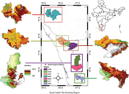
The SITR are situated in the Western Ghats of peninsular India and covers three states, Tamil Nadu, Kerala and Karnataka, latitude ranging from 75.36 to 77.09N and longitude from 9.57 to 13.35E where fragmented segments or part of the administrative district only tea is cultivated (Figure 1). The altitude of the region starts at an elevation of 630 m (KOP) to 1790 m (CNR) above mean sea level. The climate of the regions is characterised by humid tropics with cool summer with heavy rainfall, which is heavier to the south and extends over six to eight months in a year. Such a climate favours tea production under rainfed so much that accounts, one-fifth of the total tea plantations of the country with an average yield of 2281 kg ha⁻¹ and annually produces ~25% of India’s tea (Tea Board, 2016). SI is a key tea-growing region produces 243.71 Mkg (million kilogram) from 106.85 thousand hectares and exports ~36% (worth of ~157 million US$) of total annual production. Agricultural activities will take place around the year and the crop will be harvested once in the 15–21-day interval. Unlike North Indian, the SI tea gardens show bimodal cropping seasons (i.e.) First crop season during April to June and the second crop season during September to November and it peaks respectively in the months of May and October. The total annual tea productivity of the SI ranging from 2030 (VPR) to 2909 (KOP).

Figure 1. Map of elevation range and meteorological stations in the SITR. Black lines with the cross line are the boundary of tea growing region, grey lines are administrative boundaries of districts and blue line are state boundaries of India. The base map of India including administrative units at different levels was acquired in vector format with data available from GADM database of Global Administrative Areas (http://gadn.org/country) and processed using ESRI® ArcMap Version 10.1.

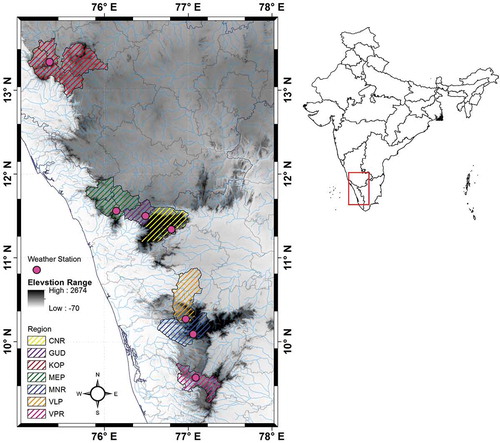
Seven meteorological stations, Coonoor (CNR), Gudalur (GUD), Koppa (KOP), Meppadi (MEP), Munnar (MUN), Valparai (VLP) and Vandiperiyar (VPR) are chosen as a representative sample of the climate in the study area (Table 1). Weather condition of the regions is influenced by the monsoon rain-belt with the highest rainfall is intense during June to September and even November in some years with large local variation because of orographic effects. According to 35-year of daily data (1981–2015), the tea growing regions of SI receives an average annual rainfall from 1,777 to 4,051 mm. About 66% of the annual rainfall occurring in the Southwest monsoon, one of the important seasons over the tea-growing regions. The Northeast rainfall accounted ~21% and remaining ~14% of rainfall occurred during pre-and-post monsoon. Among the tea growing regions the mean annual air temperatures, both Tmin and Tmax were maximum at KOP and minimum in MNR and CNR. The mean annual relative humidity (RH%) range between 78 and 91% at 830h and from 67 to 77% at 1430h. Estimated average evapotranspiration (ETo) of the region is about 88–120 mm.

Table 1. Location of weather stations and data summary of the tea growing districts of South India

Locations	Code	Lat	Log	MSL	YPH	Tmax	Tmin	RH830	RH1430	RF	Rday	S	Sday	W	S830	S1430	Sm	ETo	Cloud
Coonoor	CNR	76.80	11.34	1790	2114	22.2	13.8	78	75	1777	89	6.17	323	1.59	18.1	18.2	0.76	100	2.04
Gudalur	GUD	76.49	11.50	815	2667	27.0	14.5	87	72	2173	116	8.32	272	1.89	12.8	12.9	0.80	106	1.82
Koppa	KOP	75.36	13.53	630	2699	29.7	20.2	85	67	2186	130	7.32	284	1.80	27.9	28.0	0.76	119	2.11
Meppadi	MEP	76.14	11.56	815	2146	28.6	18.4	91	72	2843	135	8.27	342	1.96	26.3	26.4	0.82	120	2.04
Munnar	MUN	77.06	10.09	1467	2077	22.3	12.7	91	77	4051	149	5.22	274	2.08	9.4	9.5	0.85	88	2.30
Valparai	VLP	76.97	10.27	1064	2417	25.8	15.9	88	74	3822	160	6.05	290	1.30	15.1	15.3	0.82	97	2.19
Vandiperiyar	VPR	77.09	9.57	860	1874	27.1	18.1	91	72	1825	131	5.00	269	1.90	16.6	16.7	0.81	95	2.09

Values are annual means of meteorological variables and total yield calculated across all years for each location. MSL: Mean above sea level (m); YPH: yield per hector (kg ha⁻¹); Tmin: temperature minimum (°C); Tmax: temperature maximum (°C); RH830h; relative humidity at 830 h (%); RH1430h: relative humidity at 1430 h (%); RF: Annual total rainfall (mm); Rday: mean number of rain day in a year (if $>$0.20 mm day⁻¹); S: sunshine hour (h); Sday: mean number of sunny days in a year (if $>$0.10 h day⁻¹); W: wind speed (km day⁻¹); S830: minimum soil temperature (°C); S1430: maximum soil temperature (°C); Sm: Soil moisture (%); ETo: evapotranspiration (mm); and Cloud: cloudiness (%).

2.2. Data collection and definition

For the study, meteorological data recorded by the UPASI Tea Research Institute and its Regional Centres are used (UPASI Annual Reports 1981–2015), which is the longest period continuous data across the region is currently available. The rain gauges are provided by the India Meteorological Department (IMD, Chennai), and the Department personnel inspect these gauges and undertake quality control of the data. Reference evapotranspiration (ETo) and cloudiness are calculated according to Penman-Monteith (Allen, Pereira, Raes, Smith, & Ab, 1998) and Black (1956) methods, respectively, by using SPEI and EcoHydrology Packages of R Statistics. Soil temperature at 830h and 1430h and soil moisture were derived from daily values input to the Java Newhall Simulation Model (jNSM) Version 1.6.1 (NRCS, 2016). All meteorological records were subjected to a visual inspection of reasonableness, completeness and any obvious discontinuities. After quality control of data, the daily values aggregated into monthly, seasonal and annual series. The crop production data at different temporal scales across the regions for the agricultural years 1981–2015 have been collected from the various sources viz., Annual Reports of Tea Board (1981–2005), J Thomas Tea Statistics and Theillai, UPASI monthly advisory circular (2010–2015) publications. The productivity of tea is referred as the ratio of the area harvested and the dry weight of the yield.

Figure S1a shows that the total tea production of SI steadily increased due to institutional (crop genetics) and technological developments (management techniques). As many non-climatic factors influence the crop production rapidly with time, a low-pass filter (Handler, 1984) have been used to separate the long-term changes from the short-term inter-annual variations about the trend (Press, Teukolsky, Vetterling, Flannery, & Ziegel, 1987). The low-frequency (long-term trend) values are got by using a Hamming-type filter followed by applying five points Gaussian moving average. But, the person who reads should consider that it does not exactly remove the technology renovation trend over the years, but it is the best way to exclude the effect of other factors on historical yield change but the climate effects. In order to avoid the spurious effect in the models, stationarity of the data was checked before performing the analysis. Outliers, random walk, drift, trend, or changing variance in the time series is removed by transforming the data using the Augmented Dickey-Fuller (ADF) test and the KPSS test.

3. Statistical models

3.1. Multiple regression analysis (MLR)

In this study, MLR is used to find structural relations of the tea yield by assessing the complex multivariate connections with the independent climate variables. The MLR equation takes the following form:

$y_t={\beta }_0+{\beta }_1{X}_1+{\beta }_2{X}_2+\cdots +{\beta }_n{X}_n+{\epsilon }_t$

where $y_t$ is the dependent variable tea yield in year $t$, ${\beta }_0$ is the constant value or intercept of the regression line, ${\beta }_{\left(1\cdots n\right)}$ is a vector of independent climate variables and ${\epsilon }_t$ is the stochastic error term which is distributed as normal with mean zero. The contribution of one or more specific risk factors which has most influenced the tea yield of the region is assessed by the step-wise multiple regression method (SMLR) by combining a forward selection with backward elimination method. Then the variance inflation factor (VIF) was calculated in determining the multicollinearity, as $VIF=\frac{1}{\left(1-r_i^2\right)}$ where $r_i^2$ is the multiple determination coefficient obtained from $X_i$ regression on the $K-1$ independent variables residual. If $VIF=1$, no intercorrelation exists between the independent variables; if VIF stays within the range one-to-five, the corresponding model is acceptable; if $VIF>10$, the corresponding model is unstable. The choice of the final equation is based on the coefficient of multiple determination $R^2$, $F$ value of the regression coefficients and the value of the T-test.

3.2. Seasonal ARIMAX

The autoregressive integrated moving average (ARIMA) model is a stochastic model (Hamilton, 1994), which has been widely used for modelling and projecting climatological applications. The ARIMA can be written as $ARIMA\left(p,d,q\right)$ where $p$ represents the order of autoregressive processes, $d$ represents the order of difference, and $q$ represents the order of the moving-average lags. This model can be extended to account for seasonal fluctuations, with the expression $ARIMA\left(p,d,q\right)(P,D,Q{)}_s$, where $s$ indicates the length of the seasonal period. Box and Jenkins introduced the SARIMA model consists of three iterative steps: identification, estimation, and diagnostic checking (Box, Jenkins, Reinsel, & Greta Ljung, 2015). The quantitative form of an ARIMA model can be expressed as:

$y_t=\sum _{t=1}^p{\phi }_i{y}_{t-1}+{\epsilon }_t+\sum _{j=1}^q{\theta }_j{\epsilon }_{t-j}$

where $p$ and $q$ are the orders of AR and MA terms respectively, in which $y_{t-1}$ is the current and previous incidence of the time series, ${\phi }_i$ and ${\theta }_i$ the fixed coefficients and ${\epsilon }_{t-j}$ is current and previous incidence residuals. The autocorrelation functions (ACF) and partial autocorrelation functions (PACF) were used to check for seasonal effects and identify plausible models using the Ljung-Box test. The residuals are further examined for autocorrelation using ACF and PACF. The model diagnostic is performed using Bayesian information criteria (BIC) and significance tests. The model with the lowest BIC values, which are statistically significant is considered a good fit model. Diagnostic plots and the Shapiro–Wilk test are used to check for normality of the residuals in the nonlinear regression. Finally, the predictions are performed by using the best fitting model.

3.3. Artificial neural network (ANN)

Models based on ANN can effectively extract nonlinear relationships in the data-processing paradigm that is inspired by the way biological nervous systems in the human brain (Haykin, 1994) to solve specific problems (Ghodsi, Mirabdollah Yani, Jalali, & Ruzbahman, 2012). ANN has been widely used in time series predictions because of their characteristics of robustness, fault tolerance, and adaptive learning ability (Wang et al., 2011). In this study, the multilayer perceptron (MLP) with back propagation learning rule is applied, which is the most commonly used neural network structure in ecological modelling and other allied sciences (Bocco, Willington, & Arias, 2010). Mathematically an MLP can be written as $y=\phi \left(\sum _{i=1}^n{\omega }_i{r}_i+b\right)$, where ${\omega }_i$ is the weight corresponding to the input variable of $r_i$, $b$ is the bias, $\phi$ is the activation function and n is a number of input variable (Bishop, 1995; Haykin, 1994). The entire data is divided into three data sets for training (70%), validation (15%) and testing (15%) processes. The numbers of neurons were determined by trial and error method and finally the model with the lowest RMSE, and the highest coefficient of determination ($R^2$) is selected as the best-fit model. In this study, ANN models are performed using MATLAB software package (MATLAB version R2015a with neural network toolbox). A Levenberg-Marquardt (LM) algorithm based ANN model is prepared using a MATLAB code and the change of training weights $W$ is computed as follows:

$\mathrm{\Delta }{W}_k=-\left[J_k^T{J}_k+{\mu }_{k}I\right]-1J_k^T{\epsilon }_k$

Then, the update of the weights can be adjusted as follows: $W_k=W_k+\mathrm{\Delta }{W}_k$, where $J$ is the Jacobian matrix, $I$ is identify matrix, $\epsilon$ is the network error, $\mu$ is the Marquardt parameter which is to be updated using the decay rate $\beta$ depending on the outcome. In particular, $\mu$ is multiplied by the decay rate $\beta (0<\beta <1)$ whenever $E\left(W\right)$ decreases, while $\mu$ is divided by $\beta$ whenever $E\left(W\right)$ increases in a new step (Ham & Kostanic, 2001).

3.4. Multivariate vector autoregressive model (VAR)

The VAR is one of the straightforward and easy to use multivariate time series model developed by George Box and Gwilym Jenkins (Lütkepohl, 2005). The study used a VAR model to provide useful heuristics for understanding the empirical causal relationships between climate variables and tea yield. The main advantage of VAR is multivariate variables are both explained and explanatory variables. The model can be thought as a linear prediction model that predicts the current value of a $k$ variable based on its own lagged values $\left(t=1,\cdots ,T\right)$ and the lagged values of the other variables. A basic autoregressive model of order $k$ is defined as:

$y_t=c+A_1{y}_{t-1}+A_2{y}_{t-2}+\cdots +A_p{y}_{p-1}+{\epsilon }_t$

where $c$ is a $k\times 1$ vector of constants (intercept), $A_i$ are $k\times k$ matrices (for every $i=1,\cdots ,p$) and ${\epsilon }_t$ is a $k\times 1$ vector of error terms. The $i$-periods back observation $y_{\left(t-i\right)}$ is called the $i^{th}$ lag of $y$. To determine the optimal order of lags to be used in VAR, the Akaike Information Criterion (AIC) was used as common selection criteria. The advantage of VAR model is to perform the Granger causality test (Granger, 1969), which determines the direction of causality among the variables in predicting the value of another variable with zero mean (Granger-cause) (Akinboade & Braimoh, 2009; Keren & Leon, 1991). If a variable $c_t$ is found to be helpful for predicting another variable $y_t$, then $c_t$ is said to Granger-cause $y_t$. Then it is useful to include variable $c_t$ as an explanatory variable in a causal model with the following form:

$y_t={\mathrm{\Delta }}_0^{y,c}+\sum _{i=1}^n{\alpha }_i^{y,c}{y}_{t-i}+\sum _{i=1}^n{\beta }_i^{y,c}{c}_{t-i}+{\epsilon }_t^{y,c}$

where $y$ is the dependent variable(crop yield) at time $t$, $c$ is climate variables, $t-i$ is lag variables, ${\alpha }_i$ and $\beta i$ are coefficients of the model and ${\epsilon }_t$ is the error term. The Granger test is conducted by testing the following null hypothesis; $H_0:\rho =0$ climate variable does not Granger cause tea yield, and $H_1:\rho \ne 0$ climate variable Granger-causes tea yield. This can be evaluated using the F-test:

$F=\frac{\left(SS{E}_r-SS{E}_u\right)/q}{SS{E}_u/n_{df}}$

Here, SEE is the sum of square errors, $n_{df}=\left(n-p\right)-2p$ is the degrees of freedom, $n-p$ is the number of equations, and $2p$ is the number of coefficients in the unrestricted model. In addition, impulse response function is used (IRF) to identify shock reactions to the climatic variables (Ji, Zhang, & Hao, 2012; Pesaran & Shin, 1998). It shows that how much the variance of the forecast errors of each variable has been explained by exogenous shocks to the other variables in the VAR (Ghatak, 1998):

$y_t=\mu +{\alpha }_j{x}_{t-j}+{\beta }_1{y}_{t-j}+{\epsilon }_t$

where $\mu$ is constants, $\alpha$ and $\beta$ are the coefficients of the models, and ${\epsilon }_t$ is univariate white noise.

3.5. Model validation

For the construction of a model, the data divided into two sets: training (1981–2010) and testing sets (2011–2015). Several criteria are used to evaluate model performance and the difference between simulated and observed data. The root means squared error (RMSE), which measures the difference between fitted and observed values, was calculated to evaluate the systematic bias of the model. The smaller the RMSE, the better the model is for forecasting:

$RMSE={\left[\frac{{\sum }_{i=1}^n{(P_i-O_i)}^2}{n}\right]}^{0.5}\times \frac{100}{\bar{O}}$

Moreover, the statistical model validated based on the statistical significance (i.e. $p$-value) where linear regression was applied to compare observed and calibrated data and the model’s explanatory power as measured by the coefficient of determination ($R^2$) for each simulation. A high coefficient of determination ($R^2$) indicates the best model performance in capturing the observed crop yield response to climate (Lobell & Burke, 2010). Furthermore, bias and accuracy of models was measured through the mean absolute percentage error (MAPE) using the formula:

$MAPE=\frac{1}{T}\sum _{t=1}^T\left|\frac{P_t-O_t}{O_t}\right|\times 100$

where $P_t$ is the predicted value at time $t$, $O_t$ is the observed value at time $t$ and $T$ is the number of predictions. In terms of the MAE and MAPE computation, the good model will have the smallest possible value of MAPE (less than or equal to 10%). The statistical significance of the regressions is calculated to compare the predictive accuracy of the proposed models according to the Diebold-Mariano test based on absolute errors. An absolute error is simply defined as $a_i=\left|f_i-y_i\right|$ where $f_i$ stands for a estimated value and $y_i$ is an observed value. The null and alternative hypotheses are defined as: $H_0=E{\left\{{\epsilon }_t^1\right\}}_{t_0}^T=E{\left\{{\epsilon }_t^2\right\}}_{t_0}^T$ and $H_1=E{\left\{{\epsilon }_t^1\right\}}_{t_0}^T=E{\left\{{\epsilon }_t^2\right\}}_{t_0}^T$. Statistical significance was set to two-sided $p<0.05$. Finally, cross-validation plot of time series of actual and predicted values was used to assess model validity.

3.6. Sensitivity and uncertainty analyses

Additionally, the sensitivity analysis (SA) was implemented to illustrate how the variation of the output of a model can be apportioned to different sources of input (Saltelli, Chan, & Scott, 2000). Parameter sensitivity analysis at the regional level represents the influence of climate variability and other regional factors on crop yield. This would allow the selection of the most sensitive parameters for model calibration and improve the accuracy of the model at the regional scale. The first-order (FS) and global sensitivity (GS) indices were calculated for seven SITR using the Sobol’s algorithm proposed by Saltelli et al. (2000). FS provides a measure of the direct importance of each parameter, and the larger the FS index the more important the parameter. On the other hand, the GS index is a measure of the total effect of each parameter, i.e., its direct effect and all the interactions with other parameters. If the FS index is equal to the GS index for a given parameter, it means that this parameter does not interact with the other parameters. Conversely, if the FS index is lower than the GS index, it indicates strong interactions between this parameter and other parameters. With $k$ quantitative input factors, the decomposition of the variance $Var\left(\stackrel{⌢}{Y}\right)$ generalises to:

$Var\left(\hat{Y}\right)=\sum _{i=1}^k{D}_i+\sum _{1\le i\le j\le k}^k{D}_{ij}+\cdots +D_{1,2,\cdots ,k}$

where $\hat{Y}$ is the total variance (the variance of the model output), $D_i$ is the FS (local) index of the parameter $i$, $D_{ij}$ is the second-order sensitivity index for the interaction of parameters $i$ and $j$, and $S$ is the total (global) sensitivity index measure the interaction effect of many parameters $i$ (Makowski, Naud, Jeuffroy, Barbottin, & Monod, 2006; Wu, Fushui, Chen, & Chen, 2009). The sensitivities of each parameter are defined by:

$S_i=\frac{V_i}{v},S_{ij}=\frac{V_{ij}}{V},S_i=\frac{V_{ijm}}{V}\sum _{i=1}^k{S}_i+\sum _{1\le i\le j\le k}{S}_{ijm}+\cdots +S_{1,2,\cdots ,k}=1$

where $S_i$ is the FS index for the parameter $i$, $S_{ij}$ is the GS index for the interaction of parameters $i$ and $j$, and $S$ is the total GS index for parameter $i$ (the sum of all effects (first and higher order) involving parameter $i$) (Makowski et al., 2006; Wu et al., 2009). For example, if there is a three-factor model, the three total effect terms for $STi$ are:

$S{T}_1=S_1+S_{1,2}+S_{1,3}+S_{1,2,3}$

where $Si$ is simply the fraction of the variance of that value to the total variance of the model, as previously defined. Although the sum of the individual effect terms will add to one, the sum of all the $S{T}_i$ values is typically larger than one because interactions are counted multiple times. The elementary effects of each factor was computed using Monte Carlo integration based upon Saltelli’s efficient latin hypercube sampling (LHS) scheme for the estimation of standardised sensitivity indices. Specifically, 35-year time series of datasets resampled to create 5,000 simulations per parameter leading to a total number of model runs of $14\times 5,000=70,000$ to compute the FS and GS indices. The analyses were conducted using R package tgp based on 95% confidence interval.

4. Results

4.1. Region tea yield variability

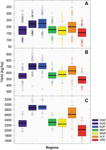
The coefficient of variation (CV) of tea yield represents the ability of the crop production system to adapt to environmental change in different regions. If the CV is near zero, crop production is considered stable while higher the CV is higher interannual variability (Zhang, Patuwo, & Hu, 1998). A box plot was used to depict the discrete levels of yield data (Figure 2). The highest coefficient of variation in CNR indicates the greatest relative variability of tea yields at the month, season and annual temporal scales. While the coefficient of variation in tea yield was marginal or less in GUD and KOP. The standard deviation (STD) of tea yields over the analysis period indicated the large interregional and interannual variability. The average yield variability (STD) was $\sim$46, 84 and 225 kg ha⁻¹ y⁻¹ respectively at the month (24.3%), season (14.1%) and annual (9.3%) scales over the study period. High annual STD up to 353 kg ha⁻¹ in tea yields was found in CNR followed by MNR while the lowest variability is obtained for GUD (155 kg ha⁻¹).

Figure 2. Crop variability in terms of coefficient of variation (CV%) and standard deviation (STD) for monthly (a), seasonal (b) and annual tea yield (c) over SITR for 1981–2015. The horizontal line in the boxes indicates mean (thick) and median (thin) tea yield (kg ha⁻¹), the lower boundary of the box indicates the standard deviation (STD) while the upper boundary of the box indicates 95% percentiles. The lower and upper whiskers representing the minimum and maximum observed value. Filled circles at both below and above the whiskers indicate outliers. Values at the bottom represent the percentage of coefficient of variation (CV) is the ratio of the standard deviation to the mean.

4.2. Comparison of models

The study establishes where and by how much crop yields varied within each tea growing regions and then identified how much of the variation in tea yields was explained by climate variables. The efficiency of the models, observed values at various temporal scales were compared with the results obtained by the SMLR, SARIMAX, ANN and the VAR. These regression equations of all the models are presented in table S1-S4. Though all possible regression combinations were attempted, only the best combination results are summarised in Table 3. Figure 3 shows the observed and predicted monthly yield for the calibration (Figure 3(a)) and the validation (Figure 3(b)) of VLP for all four models. It can be determined from the given graph that the predicted values of the calibration period show relatively good agreement with the observed values where ANN and VAR models outperform SMLR and SARIMAX models in general. Validation also has given near to the observed values with predicted values. It has been observed that the coefficient SMLR and SARIMAX during the testing period found in lower than the calibration period, except sometimes. However, the coefficient was greater during the testing period than the calibration period in the ANN and VAR models that were found to be precise models in elucidating tea yield in the peak and low cropping months/seasons. Figure 3(c) shows the scatter plot of the observed versus predicted values for the tea yield. The plot approximates a straight line, and an angle close to 45° (one-to-one line) indicates the high accuracy of the ANN and VAR models for the estimation of the tea yield for VLP.

Table 2. Coefficient of multiple linear regression

Region	Tmin	Tmax	RH830	RH1430	RF	Rday	S	Sday	W	S830	S1430	Sm	ETo	Cloud	${\mathbf{R}}^{\mathbf{2}}$
Month
CNR	37.9***	−18.5***	5.78	7.05	0.36	1.13	−0.04	2.47**	−645.9	945.7***	−959.1***	175.6***	−0.40	−52.1***	0.438
GUD	0.99	1.49	6.97	7.41	0.30	−0.73	−12.9	2.78	−626.4	75.94	−73.59	−14.12	−0.38*	5.70	0.398
KOP	21.4***	−21.6***	9.52	9.53	0.40	−0.20	8.57*	1.19	−719.0	−366.2	369.3	−42.88	0.45	−59.6***	0.448
MEP	7.44***	−11.3***	−3.81	−2.35	−0.28	0.17	−6.06	1.84	447.2	26.24	−25.89	−369.2	−0.03	−30.5***	0.156
MNR	10.8***	6.86*	5.99	7.95	0.36	−1.22	−3.48	−0.96	−691.0	−326.0**	330.9**	128.6	0.32	−5.61	0.365
VLP	6.01***	30.4***	31.00***	2.44***	−0.02*	−1.35*	−13.3***	0.24	−2703***	−571.5*	563.5*	68.03	0.64	−20.1***	0.542
VPR	17.3***	−6.62**	−4.73	−5.05	−0.30	−0.20	0.98	1.46**	507.6	−169.6	170.1	−148.8	−0.21	−14.5**	0.389
Season
CNR	72.3**	−61.2**	−5.15	−7.19	−0.18	1.55	−23.8	1.30	653.8	1577.9*	−1596.3*	480.9*	1.30	−147.1**	0.295
GUD	0.83	5.85	−18.7	−17.9	−0.44	−0.57	−120.9*	8.23**	1663.6	165.03	−162.16	−20.46	−0.90	31.02	0.136
KOP	15.6	−24.9	13.8	10.7	0.17	2.57*	63.9**	0.78	−845.9	−1664.5	1678.5	−294.5	−0.76	−51.10	0.318
MEP	−38.8***	10.8*	−5.03	−6.75	0.00	0.76	1.40	0.48	134.7	−935.10	935.80	801.6	−84.53***	1.93	0.123
MNR	5.30	3.80	4.65	11.8	−0.07	1.04	−19.3	−0.11	617.0	−2106.0***	2129.0***	−3593.0	3.41	−22.87	0.319
VLP	−11.1	68.2**	55.4***	5.81*	−0.01	−0.40	−0.36	−0.60	−4330.0***	−242.90	237.40	−241.5	−1.90	−9.547	0.286
VPR	21.0*	−28.1*	4.89	5.06	−0.05	0.34	−17.0	1.26	−282.7	1328.0	−1311.0	370.0	2.75	−12.44	0.287
Annual
CNR	223.2	−473.8	−8.40	−115.5	−0.17	6.09	−566.6	4.86	6583	−15,150*	15,280*	1096	81.5	−916.6*	0.344
GUD	72.33	9.585	6.39	7.956	0.29	−0.84	1807.9*	−34.0*	−1058	−1028	963.2	−489.4	−6.92	54.43	0.031
KOP	89.61	−641.8	−6.30	−25.38	0.39	1.55	323.7	2.13	2178	3309	−2787	−2677	−21.3	−893.4	0.612
MEP	41.98	−69.16	79.2	109.5	−0.54	2.77	314.5	5.10	15,260	−5100	5035	−56,820*	−4.82	−25.44	0.392
MNR	126.4	69.79	−67.3	−73.18	0.60	4.77	−87.0	1.67	−12,640	−19,570	19,660	32,870	13.22	−457.8	0.480
VLP	−234.5	913.4*	194.9	65.81	−0.10	0.01	1528.0*	−5.68	−18,800*	9097	−8958	−7103	−247.0*	−191.7	0.550
VPR	311.2	−195.3	−10.0	−6.696	−0.45	7.35*	−162.0	5.61*	−885	6097	−6236	7649	21.0	−38.42	0.317

$R^2$: Regression coefficient; RMSE: Root means squared error; MAPE: mean absolute percentage error; $r$: correlation coefficient; All other designations are the same as those in the footnotes below Table 1.

Table 3. Predictive performance of statistical models during calibration and testing periods for the crop yield of SITR

Region	Month							Season							Annual
	${\mathbf{R}}^{\mathbf{2}}$	Calibration Period			Testing period			${\mathbf{R}}^{\mathbf{2}}$	Calibration Period			Testing period			${\mathbf{R}}^{\mathbf{2}}$	Calibration Period			Testing period
		RMSE	MAPE	r	RMSE	MAPE	r		RMSE	MAPE	r	RMSE	MAPE	r		RMSE	MAPE	r	RMSE	MAPE	r
SMLR
CNR	0.452	33.7	15.0	0.67	33.1	16.1	0.67	0.233	68.1	9.87	0.47	49.7	7.06	0.64	0.227	172.0	5.98	0.58	38.8	1.14	0.13
GUD	0.028	36.8	13.0	0.13	32.9	12.8	0.52	0.103	80.5	9.08	0.10	52.8	6.34	0.09	0.327	147.4	4.36	0.26	137.5	3.75	0.69
KOP	0.473	34.9	12.9	0.65	35.0	11.8	0.75	0.357	67.9	7.94	0.01	51.5	5.59	0.24	0.785	60.8	1.82	0.60	118.6	3.15	0.95
MEP	0.175	33.4	15.0	0.41	40.8	18.7	0.50	0.067	65.1	9.30	0.22	64.3	9.14	0.37	0.483	136.6	4.51	0.77	80.7	2.81	0.29
MNR	0.382	37.6	17.4	0.65	50.3	24.1	0.46	0.377	70.3	10.2	0.28	78.9	9.00	0.06	0.570	190.0	7.51	0.20	69.0	2.64	0.46
VLP	0.556	36.7	14.7	0.79	50.1	25.3	0.41	0.346	90.6	11.5	0.34	71.0	9.36	0.14	0.401	271.0	8.25	0.30	260.1	7.59	0.00
VPR	0.398	30.4	17.3	0.67	42.2	20.3	0.46	0.347	61.8	10.9	0.41	70.5	10.8	0.21	0.382	204.6	8.94	0.51	112.4	4.86	0.57
ARIMAX
CNR	0.640	28.5	12.6	0.78	23.3	10.9	0.86	0.700	59.7	8.67	0.63	47.1	6.69	0.65	0.790	137.2	4.83	0.15	71.6	2.79	0.38
GUD	0.700	24.9	9.2	0.75	27.8	10.5	0.63	0.490	60.3	6.43	0.11	41.6	4.65	0.25	0.740	160.6	4.38	0.11	107.1	3.46	0.23
KOP	0.710	34.5	12.6	0.68	31.9	10.5	0.79	0.620	69.1	8.24	0.13	49.8	4.97	0.20	0.680	165.7	4.06	0.53	120.9	2.70	0.67
MEP	0.700	27.2	12.0	0.70	31.1	13.8	0.73	0.860	52.1	7.37	0.20	52.9	7.70	0.07	0.690	100.3	3.58	0.98	74.5	2.69	0.62
MNR	0.850	31.1	14.4	0.78	35.8	14.2	0.75	0.910	48.1	7.22	0.34	62.7	8.00	0.02	0.770	126.8	4.62	0.32	89.5	2.66	0.98
VLP	0.810	33.8	13.5	0.83	31.4	13.2	0.79	0.920	67.3	8.95	0.36	70.8	9.30	0.35	0.820	145.0	4.32	0.82	149.7	4.36	0.25
VPR	0.600	25.5	13.0	0.79	26.1	12.1	0.83	0.770	218.2	30.5	0.28	192.0	27.5	0.20	0.790	361.8	16.20	0.47	236.8	9.39	0.42
ANN
CNR	0.916	17.9	6.79	0.93	24.0	9.18	0.86	0.794	63.2	8.67	0.64	62.6	9.01	0.43	0.642	73.4	2.22	0.83	120.9	3.08	0.98
GUD	0.864	20.1	4.34	0.86	15.7	3.23	0.90	0.800	50.4	3.47	0.12	20.1	1.96	0.47	0.524	189.0	3.12	0.82	60.5	1.42	0.73
KOP	0.912	20.7	5.17	0.90	21.6	5.16	0.93	0.857	41.7	2.52	0.09	19.0	0.92	0.25	0.830	92.7	2.26	0.90	79.9	1.58	0.13
MEP	0.863	19.7	5.54	0.86	23.0	5.68	0.89	0.846	46.3	3.77	0.24	30.8	3.01	0.50	0.887	101.8	2.00	0.71	31.5	0.73	0.25
MNR	0.918	18.8	6.74	0.92	26.8	7.55	0.90	0.914	37.3	3.13	0.32	21.3	1.85	0.36	0.919	85.6	2.96	0.90	163.2	3.53	0.66
VLP	0.921	24.6	6.40	0.92	19.4	5.37	0.93	0.850	53.8	5.22	0.24	70.4	6.38	0.26	0.931	113.4	3.43	0.90	51.5	1.65	0.86
VPR	0.899	20.6	7.98	0.90	20.4	7.36	0.90	0.901	34.7	3.99	0.39	22.7	3.62	0.50	0.893	142.9	3.53	0.86	58.9	1.78	0.88
VAR
CNR	0.729	21.0	9.52	0.85	19.1	8.52	0.88	0.505	42.3	6.09	0.71	35.6	5.04	0.70	0.727	107.3	3.80	0.72	86.3	3.31	0.39
GUD	0.638	21.4	7.89	0.80	21.7	8.17	0.76	0.626	48.4	5.20	0.12	42.5	4.71	0.21	0.668	108.1	2.56	0.80	85.6	2.39	0.72
KOP	0.745	21.8	7.83	0.85	24.4	8.34	0.88	0.716	23.2	2.69	0.26	21.9	2.53	0.35	0.950	76.4	1.86	0.90	59.6	1.58	0.89
MEP	0.649	23.2	10.6	0.80	26.1	11.6	0.83	0.499	45.2	6.40	0.26	38.8	5.83	0.55	0.935	57.5	1.91	0.20	44.4	1.59	0.48
MNR	0.574	21.9	10.6	0.75	24.5	9.18	0.79	0.658	50.5	7.35	0.27	56.0	7.38	0.05	0.865	98.5	3.83	0.08	57.2	1.96	0.93
VLP	0.700	24.6	9.58	0.84	25.2	10.6	0.82	0.763	41.0	5.33	0.24	41.6	5.40	0.30	0.897	105.4	3.15	0.79	87.4	3.05	0.57
VPR	0.711	19.5	10.4	0.85	22.1	10.3	0.84	0.724	37.1	6.02	0.40	54.5	8.22	0.57	0.934	68.1	2.44	0.89	52.9	2.06	0.74

R²: Regression coefficient; RMSE: Root means squared error; MAPE: mean absolute percentage error; r: correlation coefficient; All other designations are the same as those in the footnotes below Table 1.

Figure 3. Comparison of observed and modelled monthly tea yield (kg/ha; y axis) of Valparai during calibration (a) and testing period (b), and cross-validation plot at various temporal scales (c). Observed yield (kg/ha) in the x-axis (in the top and in the bottom) and predicted yield (kg/ha) y-axis (in the left and right). OBS: observed tea yield; and modelled yield by SMLR: step-wise multiple linear regression; SARIMAX: Seasonal autoregressive integrated moving average; ANN: artificial neural network; and VAR: Vector autoregressive model.

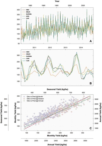
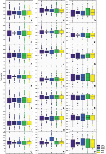
Figure 4 visually outlines the distributions of observed and estimated yield using four models. The box plot represents the 25th and 75th percentiles with the bottom and top lines of the box, respectively; the difference between these two percentiles is termed interquartile range. In addition, the line intersecting the box identifies the median of the distribution, while the two whiskers provide a measure of the data’s range. The isolated points outside the whiskers represent outliers. As can be seen in the picture, compared to the predicted yield, all models reproduce the observed dispersion of the yield quite well. As displayed by the upper whiskers, all models clearly underestimate the high levels of the yield, even though the model performs best. The performance statistics of the four different models with regard to the calibrating and testing errors for SITR are given in Table 3. All derived models are statistically significant with better model performance, except monthly and annual tea yield in CNR and seasonal yield in MEP. Even though the explained variability is lower elsewhere, the model error suggests that the climate variables have a clear impact on crop yields. Considering an average yield of 2500 kg ha⁻¹ the models have a bias of $\sim$12 to 20, 25.7 to 35 and 60 to 64 kg ha⁻¹ respectively in the month, season and annual tea yield.

Figure 4. Box Plot of observed and modelled tea yield over SITR. Left, centre and right panel shows monthly (a-g), seasonal (h-n) and annual (o-u) tea yield, respectively. The regional codes are the same as those in the footnotes below Figure 2, but for model performance.

4.3. SMLR model

The percentage of contribution of the climatic variables in the variation of tea yield was quantified by applying the MLR model and results are presented in Table 2. R² obtained by the model illustrates the fraction of the dependent variable’s (yield) variance the model could explain the response variables. The results suggest that the MRL model is able to represent the tea yield variations ranging between 3.1 and 61.2%, whereas remaining the variation is attributed to residual factors such as better clones, improved crop management operations and the introduction of modern agro-technology. The results of the MRL show that few significant relationships between yield and climate variables, these coefficients can be used to assess the real effects of climate variability in the changes in the crop yields considered in this study. In addition, the sign of the coefficients indicates the direction of change in the yield versus climate variable changes. In the most productive tea-growing region (i.e. KOP) monthly climate variability explained 44.8% of the total yield variation, at the season it was 31.8% and annual it was 61.2% (Table S1). In the low production region (VPR), climate variability explained 28.7–38.9% of the tea yield variability. In high elevation regions such as the CNR, 29.5–43.8% of the tea yield variability was explained by climate. For higher rainfall regions such as the MNR and VLP, respectively 31.9–48% and 28.6–55% of the tea yield variability was explained by climate variability.

The empirical findings revealed that the response of tea yield to the primary climatic variables, Tmin, Tmax and RF differs temporally and spatially. Tmax has a negative impact on yield at CNR, KOP and VPR in all temporal scales, whereas the seasonal and annual Tmin and RF have a negative impact on tea yield at VLP. Although temperature variability in SITR was more important, rainfall variability explained only part of the tea yield variability. Overall estimates among the primary climatic parameter indicated that Tmax had a negative influence (55.53 kg ha⁻¹ y⁻¹), Tmin had a positive influence (90.03 kg ha⁻¹ y⁻¹) and RF had an unbiased response to tea yield (0.003 kg ha⁻¹ y⁻¹). If we consider regression coefficients of the linear model represent yield increments per unit of weather change (e.g., kg ha⁻¹ y⁻¹) by holding other variables constant, a 1 °C rise in Tmin can reduce maximum 234.5 kg ha⁻¹ in the annual yield at VLP and Tmax by 641.8 kg ha⁻¹ at KOP.

4.4. SARIMAX models

According to Box-Jenkins, AR models is of second order for GUD, MNR, VLP and VPR, while, AR fourth order for CNR, KOP and MEP monthly data. For MA models, the orders are GUD MA(2), CNR, MNR, VLP and VPR MA(1) and for KOP and MEP MA(0). Also, the results show I(0) for CNR, GUD and VLP, and I(1) for KOP, MEP, MNR and VPR. The orders of SARIMAX models determine the dynamic relationship of past values of climate varies from two to four months. Analytical estimations of SARIMAX models are presented in table S2. The Ljung-Box statistics were used to check the adequacy of the tentatively identified model. The p-value of the Ljung-Box statistics was $\sim$0.405, 0.652 and 0.535 for values of lags equal to 12, 4 and 2, respectively. This indicated that the model was adequately captured the correlation information in the time series. Moreover, the residuals of the individual sample examined using the autocorrelation (ACF) and partial autocorrelation (PACF) function supported the model adequacy.

4.5. ANN models

A major issue in using neural networks is the selection of network architecture and appropriate patterns of input data that are likely to influence the desired output. After splitting the dataset into training and testing data, different learning rates, learning algorithms and the number of neurons in the hidden layers determined by the seasonal period of the time series. The optimum number of neurons was equal to one more than twice the number of input variables, i.e. $2n+1$, where $n=16$ in the study. The results suggest that the ANN is effective in reproducing nonlinear interactions with fourteen input variables, one hidden layer with twenty-five neurons and an output layer with one-output variable (14–25-1 structure). Trial and error method was followed to find out the optimal number of input delay, where maximum 3–12, 1–4 and 1–3 periods are the delays for the month, season and annual time series, respectively. The network configuration, the number of iterations, as well as the smallest global error achieved within the specified number of iterations and training run-time which are given in table S3. The results were compared with actual observations by means of time series analysis and scatter statistics (scatter points, RMSE, MAPE and Pearson correlation coefficient). Figure 3 shows the scatter plot of the observed versus predicted values where the plot approximates a straight line, and an angle close to 45° (one-to-one line), which indicates the high accuracy of the ANN model for the estimation of tea yield.

4.6. VAR models

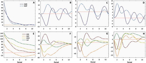
In the present study adopted a multivariate VAR model with exogenous variables because of lesser forecasting errors. The number of lags for VAR model is restricted from 5 to 12 for the month, 3 to 5 for the season and 1 for the annual dataset which was chosen by basing on AIC and HQIC criteria, i.e., the minimum AIC and HQIC. The results of the VAR model and SIC criteria are presented in table S4. In Figure 5, the vertical axis is the impulse responses of the yield, and the horizontal axis is the lag time (year) after the initial positive impact are applied to independent climate variables.

Figure 5. Impulse response functions of climate variables on tea yield (y-axis), Response of YPH (a & e), Tmin (b & f), Tmax (c & g) and RF (d & h) at seasonal (a-d) and annual (e-h) time series.

4.7. Monthly tea yield response to climate variation

Figure 4 illustrates the performance of the modelled yield compared with the observed yield. The models are adequate to explain $\sim$2.8 to 92.1% of the total variance of monthly tea yield with 4.34 to 17.4% and 3.23 to 25.3% MAPE during training validation periods, respectively. Based on the performance of the models (i.e. RMSE, MAPE) and the Diebold-Mariano test, ANN found to be a best-fit model for monthly tea yield of all the regions because of their strong nonlinear mapping ability and tolerance to complexity in data. The model captured both mean and outlier values efficiently as well. The application of the ANN model in predicting monthly tea yield, climate variables explained $\sim$86.3 (MEP) to 92.1% (VLP) of variation. That leaves the average MAPE between $\sim$6.1 and 5.5% during the calibration and testing periods, respectively.

The application of ANN model explained highest 92.1% of yield variation in the VLP region ($YPH\sim =0.97\times Target+6$) obtained with four months delay period and the model structure is 14–25-1. For KOP ($YPH\sim =0.80\times Target+50$), CNR ($YPH\sim =0.89\times Target+16$) and MNR ($YPH\sim =0.93\times Target+13$), the model explained $\sim$91% of yield variation (14-23-1 structure) with information from three months delay period. The best prediction for MEP, GUD and VPR regions was obtained (14-21-1) with information from the past five months with $\sim$20 kg ha⁻¹ (6%) error during the calibration and testing period. The delay period of the model 3–5 months shows that the yield was strongly influenced by the earlier month weather condition or the prediction of the yield could be possible in advance to the current month.

4.8. Seasonal tea yield response to climate variation

For seasonal tea yield, response variable able to explain 7% (MEP) to 38% (MNR) by SMLR, 49 (GUD) to 92% (VLP) by SARIMAX, 79 (CNR) to 91% (MNR) by ANN and 92.5 (KOP) to 99.6% (VLP) by VAR. Among the four models, the performance of the ANN found to have the strongest explanatory ability in explaining seasonal tea yield variation of GUD, MEP, MNR and VPR tea-growing regions (Figure 4). While the VAR model for CNR and KOP, and SARIMAX for VLP found to best-fit model for the seasonal yield.

The model structure of seasonal tea yield for GUD is 14-21-1 with the information of three-season delay period resulted in the least error during the calibration (3.47%) and testing (1.96%) periods and explained 80% of seasonal yield variation. For MEP, the model ($YPH\sim =0.99\times Target+8.9$) structure (14-23-1) explained 84.6% of yield variation with four months delay period. The ANN model for MNR ($YPH\sim =0.92\times Target+49$) elucidated 91.4% of variation associated to climatic variables with a model structure 14-11-1 and four delay periods. In case of the VPR region, the model ($YPH\sim =0.92\times Target+38$) with two delay period explained 90.1% of variation shows the lowest training and testing error.

The effects of the climate variables on the seasonal tea yield (CNR and KOP) assessed using the VAR model is statistically significant ($p<0.001$). The $R^2$ value indicates that 50.5 and 71.6% of the variation are explained by climate variables of CNR and KOP, respectively. The result shows that meteorological data included in the model are sufficient to explain regional and other complex factors that influence tea yield. F-statistic shows that the lagged terms four for CNR ($F=7.767;p<0.001$) and two for KOP ($F=8.972;p<0.001$) were statistically significant. The results from Table 4 show that there was a strong causal relationship between climate variables and tea yield. The null hypothesis in each case assumes that all the climate variables included in the model “Granger-cause” the yield, except RH830 at KOP. Since the F-statistic was statistically significant and the direction of causality from climate variables to yield, it is necessary to observe that the IRF which allows us to examine the yield responses to shocks. As seen from the Figure 5, crop yield reacts to impulse (shock) in Tmax, Tmin and RF for twelve periods. According to the Figure 5(a) about IRF from yield to its own, increasing of the yield in the current period has a positive effect on per hectare in the future, and show a decreasing trend of positive effect up to seven periods. The dynamic relationship of climate variables to yield, increasing of Tmin, Tmax and RF in the current period positively influence yield up to six periods for KOP and shows a gradually decreasing trend with uncertain positive effects. Increasing of Tmin, Tmax and RF in the current period will have an uncertain positive effect on crop yield of CNR in the future. YPH decreased sharply up to three periods and there is a brief upward after four and eight periods.

Table 4. Granger causality test

Month	CNR	GUD	KOP	MEP	MNR	VLP	VPR
Tmax	16.8***	4.62***	3.14***	5.31***	4.44***	5.49***	8.65***
Tmin	14.4***	2.85**	1.84**	6.76***	4.36***	12.6***	14.4***
RH830	7.06***	0.32^ns	0.73^ns	3.43***	2.95**	2.28**	5.07***
RH1430	11.9***	0.31^ns	1.19^ns	2.54**	3.48***	9.75***	5.14***
RF	6.53***	2.10*	2.17**	6.97***	5.73***	9.46***	10.8***
Rday	11.8***	1.50^ns	2.53***	6.84***	5.25***	10.4***	9.75***
S	8.67***	1.96*	4.56***	6.71***	9.62***	9.88***	6.31***
Sday	4.65***	2.33**	2.06**	8.36***	6.19***	10.2***	7.12***
W	10.4***	1.14^ns	1.45^ns	5.99***	4.81***	1.75^ns	8.83***
S830	19.6***	2.65**	3.06***	6.77***	7.19***	10.7***	3.09***
S1430	19.6***	2.66**	3.09***	6.76***	7.20***	10.7***	3.02**
Sm	6.88***	0.70^ns	1.25^ns	3.80***	3.39***	7.87***	5.83***
ETo	15.4***	1.75^ns	3.16***	7.33***	8.85***	10.2***	4.95***
Cloud	7.47***	0.61^ns	1.75*	5.57***	5.04***	7.29***	8.04***
Season
Tmax	6.15***	0.30^ns	2.63*	0.81^ns	1.52^ns	4.98***	16.9***
Tmin	5.96***	0.43^ns	2.87*	3.47**	1.88^ns	4.17***	14.8***
RH830	2.74**	0.25^ns	1.65^ns	1.41^ns	5.94**	2.70**	4.45**
RH1430	3.06***	0.48^ns	6.36***	2.76*	2.09^ns	6.19***	29.2***
RF	2.94**	0.18^ns	3.62**	4.97***	1.88^ns	4.24***	27.0***
Rday	3.67***	0.33^ns	4.54**	5.40***	1.79^ns	6.24***	21.8***
S	4.65***	0.21^ns	5.79***	5.38***	1.31^ns	5.94***	27.0***
Sday	3.26**	0.29^ns	3.99**	4.68**	1.77^ns	4.51***	18.5***
W	3.12**	0.32^ns	5.04***	4.15**	2.19^ns	2.18*	32.3***
S830	6.72***	1.00^ns	3.81**	4.15**	0.68^ns	3.56***	12.6***
S1430	6.72***	1.01^ns	3.78**	4.15**	0.70^ns	3.57***	13.0***
Sm	3.50***	0.27^ns	6.16***	2.72*	2.73*	5.59***	7.42***
ETo	4.50***	0.25^ns	4.82**	2.63*	1.53^ns	4.78***	19.5***
Cloud	3.46**	0.35^ns	4.67**	2.19^ns	1.78^ns	4.90***	37.5***
Annual
Tmax	1.77^ns	1.80^ns	0.25^ns	4.68**	0.30^ns	0.00^ns	0.67^ns
Tmin	0.17^ns	1.51^ns	0.40^ns	0.86^ns	0.04^ns	0.29^ns	0.33^ns
RH830	0.26^ns	0.12^ns	0.20^ns	1.64^ns	0.61^ns	0.18^ns	0.55^ns
RH1430	0.04^ns	0.30^ns	3.56*	0.73^ns	0.34^ns	3.57*	0.35^ns
RF	0.60^ns	0.15^ns	3.47*	0.71^ns	0.02^ns	0.27^ns	1.01^ns
Rday	0.10^ns	0.00^ns	0.90^ns	0.01^ns	0.03^ns	0.00^ns	14.3
S	1.32^ns	0.01^ns	5.32**	0.15^ns	0.26^ns	2.37^ns	0.87^ns
Sday	0.11^ns	0.03^ns	1.36^ns	0.39^ns	0.11^ns	0.09^ns	2.71^ns
W	0.09^ns	0.01^ns	0.30^ns	1.51^ns	0.56^ns	0.75^ns	0.26^ns
S830	0.55^ns	1.83^ns	0.20^ns	3.56*	0.27^ns	0.41^ns	0.81^ns
S1430	0.52^ns	1.92^ns	0.20^ns	3.55*	0.26^ns	0.42^ns	0.83^ns
Sm	0.06^ns	0.44^ns	0.01^ns	1.14^ns	0.64^ns	4.18**	1.10^ns
ETo	0.52^ns	0.43^ns	2.53^ns	1.01^ns	1.43^ns	1.22^ns	1.83^ns
Cloud	0.50^ns	0.30^ns	0.88^ns	3.10*	0.15^ns	0.22^ns	0.28^ns

All designations are the same as those in the footnotes below Table 1.

For VLP, the best fit model is SARIMAX(0,1,0)(2,0,0)₄ (Log-likelihood = −764.61, AIC = 1561.21; Table S2), where Tmax, Tmin, RF, Sday and Cloud are the most limiting factors negatively regulating the crop yield. All coefficients for the estimated model are significant at the 5% level. The $R^2$ value of the estimated model is 0.920, showing that $\sim$92.0% of the variation is due to a seasonal climate that could be explained by the estimated previous lag value and the lagged error terms. The RMSE of training and testing periods are 67.29 and 70.82 kg ha⁻¹, while the MAPE is 8.95 and 9.30%, relative to the average of the predicted yield of 633 kg ha⁻¹. Ljung-Box statistic value is 17.148 for 15 degrees of freedom and the significant probability corresponding to Box-Ljung Q-statistic is 0.310, which is greater than 0.05. Therefore, it is accepted and it may be concluded that the selected SARIMAX(0,1,0)(2,0,0)₄ model is an adequate model for the given time series. The correlogram and Q-statistics show that there are no significant spikes in the ACFs or PACFs at 95% confidence limits (figure not shown), which indicates that the residuals of this SARIMAX model are white noise. The forecast performance is better than the other three models while the number of inputs is kept equally for all models. Moreover, the model shows no sign of biased estimations across the entire duration of the prediction period (5 years), as suggested by the scatter plot of the predicted and the observed yield (Figure 3(c)). However, the error in the high season period is still higher than the other period like the other three models because the month-to-month and year-to-year variations of the yield are driven by many factors.

4.9. Annual tea yield response to climate variation

In case of annual tea yield variability response, the SMLR model explained 22.7 (CNR) to 78.5% (KOP), SARIMAX 68 to 82%, ANN 52.4 (GUD) to 93.1% (VLP) and VAR 66.8 (GUD) to 95.0% (KOP). This shows that the VAR and ANN models explained higher annual tea yield variability than its counterparts. The overall analysis revealed that the VAR model for GUD, KOP and VPR, and ANN model for CNR, MEP, MNR and VLP found to best fit model explains more than $\sim$84% of the interannual tea yield variability.

Based on the performance and error terms, the ANN model found to be an optimal model to elucidate the yield variability response of CNR ($R^2=0.642;RMSE=73.4$), MEP ($R^2=0.887;RMS=101.8$), MNR ($R^2=0.919;RMSE=85.6$) and VLP ($R^2=0.931;RMSE=113.4$) with reference to annual climate (Table 3). The model structure 14-23-1 with the delay period information of three for CNR ($YPH\sim =1\times Target+15$), two for MNR ($YPH\sim =1.0\times Target+0.57$) and VLP ($YPH\sim =0.91\times Target+200$) and one for MEP ($YPH\sim =0.96\times Target+110$) resulted lowest error during training and testing periods.

The appropriate number of lag of the VAR model is one for GUD ($AIC=1;F=2.133;p<0.066$), KOP ($AIC=1;F=2.536;p<0.001$) and VPR ($AIC=1;F=15.070;p<0.001$). The result signifying the existence and nature of the long-run relationships between climate variables and crop yields of three locations ($p<0.001$). $R^2$ value of the model is 0.668 (GUD), 0.950 (KOP) and 0.934 (VPR) suggesting that the variation is due to climate is significant and that could be explained by the estimated previous lag value. The Granger causality test has been checked whether significant cause, equilibrium relationships from climate variables to the crop yields in the chosen locations exist (Table 4). There is a strong causation of yields of tea and RH1430, RF and S in KOP and Rday in VPR, while no empirical evidence of causality exists from climatic variables to the yields of VPR.

Compared with the IRF response pattern of annual yield to its own (Figure 5(e)), the response of raising yield in the current period has a positive effect up to twelve periods. Exceptionally MEP has positive effects up to four periods, then extensively subdued after the shock. With rising Tmin, the yield is driven positivity in the first four periods for CNR and VLP, but there is a brief increase in CNR then drops more slowly (Figure 5(f)). While VLP declines gently to its shock and increase after almost nine periods after the shock. However, yield explodes after the two-period shock of Tmin in MNR and peaked in six periods and also maintains the positive effect for a long period accompanied by minor fluctuations. When shocked positive from Tmin on the first period, the yield drops sharply before peaking five periods after the shock and sustains negative effects for a long time. The similar trend is followed in case of Tmax in MEP. From Figure 5(g), the increment in yield reaches a maximum of about four periods after the initial Tmax shock occurs in CNR and MNR. Likewise, a shock to Tmax increases yields up to ~13.25 kg ha⁻¹ with a peak reached on two periods after the shock was applied followed by an uncertain decrease and brief increase. The effect of a shock in rainfall on yield is caused a quick decay with inducing further increment in subsequent periods while a shock in rainfall induces further increment in yield of VLP which can take about four periods to reach maximum.

4.10. Sensitivity and uncertainty of climate variables

To further investigate the influences of climate variables on tea yield, a sensitivity analysis was utilised by a variance-based bootstrap resampling technique. The analysis help to identify key parameters and rank the uncertain input factors with respect to their effects on the nonlinear statistical model output variables by calculating quantitative indices. Figure 6 shows the sensitivity indices calculated for the tea yield at various temporal scales for seven regions. The FS reflected the main (local) effect, and the GS indices reflect the sum of all effects involving the parameter on the model output, including interactions with all other criteria.

Figure 6. First order (FS: in Orange) and total global sensitivity (GS: in Red) of tea yield (kg ha⁻¹) due to climate variability at month (a-g, top panel), season (h-o, middle panel) and annual (P-V, bottom panel) scales. All abbreviations are the same as those in the footnotes below Table 1.

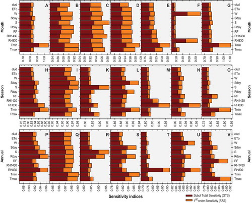
The FS of Tmin, Tmax, S, S830 and W were much higher than the other parameters which indicating the direct influence of the parameter that determined monthly tea yield. The highest FS index of Tmin registered by VPR (0.188) indicated that Tmin alone determined ~19% of the variation of the model output. Similarly, the Tmin of CNR (14%), MNR (9%) and MEP (5%) found to be a key parameter that recorded higher FS values. However, the FS of Tmin in GUD (0.053), KOP (0.040) and VLP (0.041) differed from other stations by registering lower FS values between 4 and 5%. It has been observed that the FS of S830 in GUD (0.080), S in KOP (0.053) and W in VLP exhibited the highest sensitivity indices consider as region-specific key parameters. The estimated FS for RF and Tmax were ~4 and 5%, which was on par with FS key parameter in some regions. The result indicates that even though the FS value was lower than the key parameter, RF and Tmax were equally important in influencing the crop yield. In consonance with FS, GS shows a similar pattern of the highest sensitivity towards Tmin, Tmax, S, S830 and W of the respective regions. Tmin was the most sensitive factor in four of the seven regions. The GS was highest in MEP (0.944) denoting that 94% of the variation of the model output was influenced by Tmin. When comparing FS of Tmin in MEP (0.052), reaming 89% of the variation of the model output was controlled by the interaction of Tmin with other variables. Likewise, the highest GS of Tmin recorded in CNR, MNR and VPR showed that Tmin of the region was dealt with by the interaction with other variables.

FS values based on seasonal yield, Tmin, RH830, S and S830 are found to be the key parameters by registering higher indices that are specific to regions. Tmin is the most influential factor in CNR (0.049), and VPR (0.085) followed by RH30 in MNR (0.086) and VLP (0.044), S in GUD (0.019) and KOP (0.071), and S830 in MEP (0.035). However, the primary meteorological variables Tmax and RF registered only $\sim$3 and 4% of the variation of the model output. The highest GS of Tmin in GUD (0.961) followed by RH830 in VLP (0.950) and S830 in MEP (0.915) shows that >94% of the variation where $\sim$90% of the variation of the model output was controlled by the interaction with other parameters. For the annual yield, FS shows explicit variation in key parameters. The most sensitive factor in CNR is Rday (0.030), Tmin in GUD (0.017), S in KOP (0.072), S830 in MEP (0.056), RH830 in MNR (0.172) and VLP (0.052), and Tmax in VPR (0.056). RH830 found to be the most sensitive factor besides the important key variables irrespective of regions compared. Rday and Tmax are also a highly sensitive parameter for three regions in which the global sensitivity index is highest and interaction with other parameters is usually much less than the first-order interaction.

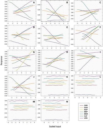
Figure 7 shows the large spatial variation in the total sensitivity of different climate variables to the variability of tea yields across SI. In general, increasing Tmin had a positive impact on yields over most of the tea growing regions, except for MEP and VLP (Figure 7(a)). In contrast, Tmax exerted a negative impact on tea yields except for MNR and VLP. Especially the negative impact was strongest in VPR regions, and it is unassertive in CNR (Figure 7(b)). An increase one standard deviation of RH830 can lead to decrease in tea yields in MNR and MEP regions (Figure 7(c)). The increase of RH1430 was found to drive up tea yield, especially in MNR and VPR while the increase in relative humidity to drive down tea yield in CNR, GUD and VLP (Figure 7(d)). Compared to the other regions, the magnitude of tea yield sensitivity to RF was larger in VPR followed by VLP (Figure 7(e)). Yield expected to increase by up to one standard deviation increase of RF in some major tea growing regions such as CNR, MEP and MNR. However, the magnitude of change is larger mid-altitude region MEP, and it was lesser in the higher altitude regions CNR and MNR. Tea yields in several SITR are most sensitive to changes in S, with a ~ 2 to 4% increase in response to a + 1 deviation increase in S of GUD, KOP, MEP and VPR (Figure 7(g)). The tea yield of VLP is more sensitive to W which shows much larger magnitude in change than in other regions (Figure 7(i)). MEP, MNR and VPR show high sensitivity to S830 where the larger positive response in MNR and VPR and negative response in MEP when an increase in S830 (Figure 7(j)). The climatic variables S1430, Sm, ETo and cloud have narrow uncertainty bounds, but vary substantially in the sign and magnitude of their influence (Figure 7(k-n)).

Figure 7. Region and variable specific global sensitivity response at month, season and annual tea productivity. (a): Tmin (°C); (b): Tmax (°C); (c): RH830h (%); (d): RH1430h (%); (e): RF (mm); (f): Rday; (g): S (h); (h): Sday; (i): W (k day⁻¹); (j): S830 (°C); (k): S1430h (°C); (l): Sm (%); (m): ETo (mm); (n): Cloud (%).

5. Discussion

Since the climate factors and their influences on tea yields found to covary on spatiotemporal scales, understanding the discrete effects of each climate factors and its uncertainty can help to develop more effective adaptation strategies in response to climate change anticipated. In line with similar studies in related domains, the present study demonstrated the use of empirical statistical modelling on observational data to understand the spatiotemporal dynamics of tea yield in response to climate. However, the reader should consider that the models do not explicitly take into account of extreme weather events (e.g. warm and cold spells, strong wind, hail, heavy or less precipitation) that may often lead to complete crop failure (Hawkins et al., 2013). Indeed, by using the time series of monthly and seasonal scales, the extreme events that act on a shorter time scale are partially reflected in the yield averages.

Among the statistical models, ANN and VAR models produced flexible and powerful results which are highly specific to each region-temporal pair. It is worth pointing out that the ANN models (for a month, season and annual yield data) ranked first in terms of training and testing performance than its counterparts (Table 3). It could be due to the nonlinear patterns in the dataset have not probably as strong impact on tea yield compared to the predictors, which are linearly related to yield. On the other hand, the training of an ANN does not use the entire available database because the test subset of data is not employed in the learning process. Generally, the performance of SARIMAX is poorer than those of ANN and VAR for most of the time series. The poor performance probably resulted because SARIMAX model assumes that time series are generated from linear processes, whereas the yield time series are often nonlinear and seasonal (Granger & Teräsvirta, 1993; Zhang et al., 1998). The SARIMAX model generally performs better when periodicity exists in the data, as the periodicity is taken into account by the model by differencing the data (Mishra, Desai, & Singh, 2007). Probably because of the lack of seasonality in the data in these months, the SARIMAX models performed poorly.

Irrespective models, the performance was better for the southern locations (MNR, VLP and VPR) than the northern locations (CNR, GUD, KOP and MEP) indicated that the relationships between climate variables and tea yield are stronger in the southern parts. Probably because of a weak relationship between the rainfall pattern in the northern locations and the climate variables. In line with the modelling efficiency, the performance of each method in terms of producing small errors varied depending on time series and locations. For instance, the MAPE for monthly tea yield was smallest with the ANN approach, whereas that for the annual yield was smallest with the VAR. In general, the variability in monthly tea yield related to climate variability was higher in VLP ($\sim$92% of the yield), followed by ($\sim$91% (CNR, KOP and MNR) of the yield variability of SITR. Approximately 77–80% of the seasonal tea yield variability was explained by climate. As highest, 80–93% of the annual yield variability explained by climate variability translates into large fluctuations in tea production. For example, in the study at an average ~84.8% of the annual tea yield variability of 1.9 t ha⁻¹ y⁻¹ explained by climate variability, over 106.85 thousand ha translates into an annual fluctuation of $\sim$0.02 million tons in tea production over the study area.

Tea cultivation in SI is not consistent with the climatology of all the regions. Climatological records in SI exhibit bimodal rainfall patterns such as Southwest (May-Aug) and Northeast monsoons (Sep-Dec). Except for CNR, all the tea growing receives $\sim$66% of the annual rainfall during the Southwest monsoon and $\sim$21% rainfall during the Northeast monsoon seasons. Thus, the tea plant is not able to capture the optimal window of growing conditions as the duration and frequency of rainfall related important other cofactors viz., relative humidity, rain day, cloud cover, sunshine hour and sunny day differed spatially. The relation between rainfall and rain day congruent with two possible patterns of impact on yield: a) increase in rainfall with higher number of rain day positively sensitive to the crop yield in CNR, MEP and MNR while it is negatively sensitive in VLP and GUD; and b) decrease in rainfall with higher number of rain day found to be sensitive to the crop yield in KOP and VPR (Figure 7(e, f)). The result confirms the importance of water availability in rainfed tea cultivation but also emphasises that the frequency of rainfall matters more than the total amount of rainfall in most of the localities (Ujjal, Joshi, & Bauer, 2015). Moreover, the influence of RF variability on tea yield was observed to be strong only in VPR and the sensitivity related to RF of all other regions found to be less than 4%. This was because tea growers of the regions are already adapted, or adapting, to climate change, which has made them also more adapted to rainfall variability. Indeed, the tea planters are suggested for developing an efficient water harvesting infrastructures in the areas where an uneven distribution of low rainfall frequency is more prevalent. Increasing in rainfall with increasing rain day found to affect yield positively in CNR, MNR and VLP were attributed to readily dissolving the soil nutrients facilitate easy absorption of the tea plants. While the negative impact of increasing rainfall with rain day in VLP was because of intense rainfall during the monsoon seasons lead to soil erosion or the washout of surface soil and the depletion of plant nutrients in soil due to runoff (Ruhul Amin, Zhang, & Yang, 2015). The lower sensitivity of annual yields of KOP and MNR was primarily because it was able to compensate for part of the yield loss that occurred during the dry period by having a substantially higher yield during the wet period of the year.

Temperature variability was found to be the most important factor for tea yield in SI due to the high availability of RF controlling the influence of RF variability, soil moisture, soil temperatures and ETo rate. This result confirms that the temperature is a more important contributor to climate change impact than rainfall (Bilham, 2011). A changing Tmax and Tmin some regions found to have beneficial (harmful) effect on crop production by enhancing (decreasing) photosynthesis, rate of shoot initiation in tea (Roberts, Summerfield, Ellis, Craufurd, & Wheeler, 1997; Squire, 1990) and the shoot growth (Carr, 1972; Carr & Stephens, 1992; Watson, 1986) thereby increasing crop yield as it increases (Ruhul Amin et al., 2015). However, the above or below optimal temperatures differentially influences the metabolic processes of tea plants by affecting the stability of various proteins and membranes, rates of photosynthesis and RuBisCo function and thereby inhibiting crop yield (Mathur & Jajoo, 2014). The inverse relationship with increasing temperature suggested that excess temperature would be detrimental to tea production where long-term effects of climate change (in relation to temperature) are larger than short-term effects.

The higher sensitivity of RH830h in MNR and MEP regions (Figure 7(c)) and RH1430h in CNR, GUD and VLP regions (Figure 7(d)) is attributed to direct and indirect control of relative humidity on crop yield. Increase in relative humidity is not beneficial for higher yield as it directly controls the plant-water relationships and absorption of soil nutrients, and indirectly influences stomatal control, photosynthetic rates, leaf water potential and the occurrence of fungal diseases. The sensitivity of S with Sday in response to yield leads to three possible patterns of impact: a) increase in S with Sday found to be either positively sensitive to CNR, KOP, MEP and VPR or negatively sensitive to GUD; b) MNR found too sensitive to decrease in S with increasing Sday; and c) VLP shows sensitivity to increasing S with decreasing Sday (Figure 7(g, h)). Sunshine hour directly affects crop growth by influencing the onset and release of bud dormancy and shoot development (Matthews & Stephens, 1998b). Excessive sunshine negatively affects crops as the temperature effects (Smestad, 2014). Some tea growing regions experience both cooler and warmer climates at a given altitude that modifies the balance between shoot and root growth by influencing the physiology of shoot growth. Cooler periods tend to result in banji formation (dormant shoots) due to the higher partition of carbohydrates to the roots while in warmer periods, carbohydrates are re-translocated to the developing shoots (Fordham, 1972; Rahman & Dutta, 1988; Squire, 1977).

In addition to air temperature, soil temperature also influences the growth of the tea plant (Carr, 1972; Carr & Stephens, 1992), especially in situations where yield is limited by higher soil temperature of the regions. Magambo and Othieno (1983) reported that high soil temperature during the daytime combined with low soil temperature during the night induced early flowering of tea and reduced the vegetative growth. Some tea-growing regions, especially VLP experience periods of high wind speeds during certain times of the year and it is found to be highly sensitive to crop production. High wind speeds generally tend to increase ETo from tea canopies extensively and thereby accelerate the development of deficit soil moisture and stomatal closure in dry periods may reduce photosynthesis. Banerjee (1993) reported that wind turbulence could reduce the high temperature, which otherwise would adversely affect photosynthesis. However, the direct effect of wind speed on the physiology of growth and productivity of tea is still unknown.

6. Limitation of the study

The study considered only climatic variables and not measured the spatial heterogeneity in climate-yield response to soil and other socioeconomic attributes that might have limited the performance of the models. In future, datasets that include variables of input and output economics, soil characteristics and management should allow the models to explain greater amounts of yield variability. Finally, to improve the spatial match between crop and climate data, geo-referenced data with sophisticated statistical models are needed to address the problem.

7. Conclusion

The study helps to describe the complex relationships between climate and yield and highlighted the crucial roles of key climatic factors that determining tea yield. Among the statistical models, ANN and VAR models produced the best fits for monthly, seasonal and annual yields, probably indicates that the multivariate time series models may be better suited for capturing the long-term and short-term variations in the time series. The developed statistical models can be easily integrated into a crop yield forecasting system under different climatic scenarios by using the probabilistic weather forecasts of the identified meteorological variables. The study also demonstrated the impact of climate variability on tea yields at spatial and temporal scales. Therefore, the study suggests the policymakers develop imperative regional specific adaptation strategies and effective management practices to mitigate the negative impact of climate change on crop yields.

Author’s contribution

EER has carried out the research design, data collection, database construction, analyses, synthesis and write this manuscript. KVR and RRK supervised the research work, reviewed the results and commented on the manuscript. All authors read and approved the final version of the manuscript.

Cover image

Source: Author.

Acknowledgements

The research reported in this manuscript was conducted while the first author was a doctoral research scholar at the Bharathiar University, Coimbatore, Tamil Nadu, and CSIR-Fourth Paradigm Institute (CSIR-4pi), NAL-Belur campus, Bangalore 560 037, India. This work was supported by the SPARK Programme of CSIR-4pi and National Himalayan Mission (NMHS-2017/MG-04/480 and NMHS-2017-18/MG-02/478). The first author thankful to Advisory Officers of the Regional Centres for making available digitised meteorological data and support from both the institutions is clearly acknowledged. The authors are indebted to Dr B. Radhakrishnan, The Director, UPASI Tea Research Foundation, Tea Research Institute, Valparai for his constant support and encouragement. The findings, interpretations and conclusions expressed in the manuscript are the authors’ alone, and they do not necessarily represent those of their affiliated institutions.

Supplementary material

Supplemental data for this article can be accessed here.

Additional information

Funding

This work is partially funded by the Ministry of Environment and Forests and Climate Change (MoEFCC), Govt. of India under National Himalayan Mission (NMHS-2017/MG-04/480 and NMHS-2017-18/MG-02/478).

Notes on contributors

Esack Edwin Raj

Esack Edwin Raj is an Assistant Plant Physiologist at UPASI Tea Research Institute, Valparai and a Doctoral Research Scholar supported by CSIR-Fourth Paradigm Institute (CSIR-4pi), Bangalore through SPARK Programme. He is interested in using various empirical spatial statistical approaches of research in understanding the linkages between climate and crop yield variability for sustainable tea production in South India. His research focus is on sustainable land use management and planning, geographical information systems, digital mapping and in developing drought tolerant and disease resistance clones using marker-assisted selection.

K. V. Ramesh

K. V. Ramesh is a Senior Principal Scientist at CSIR-4pi, Bangalore. His key research area is climate change, atmosphere, hydrology, energy and disease.

Rajagobal Rajkumar

Rajagobal RajKumar is a Senior Plant Physiologist (Ret.) at UPASI Tea Research Institute, Valparai. He is an expert in tea physiology and his research focus is on climate change, carbon sequestration, agronomy and policymaking.

References

- Adhikari, R. (2015). A neural network based linear ensemble framework for time series forecasting. Neurocomputing, 157, 231–30. doi:10.1016/j.neucom.2015.01.012
- Ahmed, S., Orians, C. M., Griffin, T. S., Buckley, S., Unachukwu, U., Stratton, A. E., … Kennelly, E. J. (2013). Effects of water availability and pest pressures on tea (Camellia sinensis) growth and functional quality. AoB Plants, 6. doi:10.1093/aobpla/plt054
- Ahmed, S., Stepp, J. R., Orians, C., Griffin, T., Matyas, C., Robbat, A., Cash, S., ... Kennelly, E. (2014). Effects of extreme climate events on tea (Camellia sinensis) functional quality validate indigenous farmer knowledge and sensory preferences in Tropical China. PLoS One, 9(10), e109126. doi:10.1371/journal.pone.0109126
- Akinboade, O. A., & Braimoh, L. A. (2009). International tourism and economic development in South Africa: A Granger causality test. International Journal of Tourism Research, 12(2), 149–163. doi:10.1002/jtr.743
- Allen, R. G., Pereira, L. S., Raes, D., Smith, M., & Ab, W. (1998). Crop evapotranspiration-Guidelines for computing crop water requirements-FAO Irrigation and drainage. 300. 56. doi:10.1016/j.eja.2010.12.001.
- Ayoubi, S., Khormali, F., & Sahrawat, K. L. (2009). Relationships of barley biomass and grain yields to soil properties within a field in the arid region: Use of factor analysis. Acta Agriculturae Scandinavica, Section B-Plant Soil Science, 59(2), 107–117. doi:10.1080/09064710801932417
- Banerjee, B. (1993). Physiology in relation to productivity. In Tea production and processing (pp. 113–124). New Delhi, India: Oxford & IBH Publishing Co., Ltd.
- Bilham, J. (2011). Climate change impacts upon crop yields in Kenya: Learning from the past. Earth & Environment, 2893, 1–45.
- Bishop, C. M. (1995). Neural networks for pattern recognition. Journal of the American Statistical Association, 92, 482. doi:10.2307/2965437
- Black, J. N. (1956). The distribution of solar radiation over the Earth’s surface. Theoretical and Applied Climatology, 7(2), 165–189. doi:10.1007/BF02243320
- Bocco, M., Willington, E., & Arias, M. (2010). Comparison of regression and neural networks models to estimate solar radiation. Chilean Journal of Agricultural Research, 70(3), 428–435. doi:10.4067/S0718-58392010000300010
- Box, G. E. P., Jenkins, G. M., Reinsel, G. C., & Greta Ljung, M. (2015). Model identification (5th ed.). Hoboken, NJ: John Wiley Sons.
- Carr, M. K. V. (1972). The climatic requirements of the tea plant: A review. Experimental Agriculture, 8, 1–14. doi:10.1017/S0014479700023449
- Carr, M. K. V., & Stephens, W. (1992). Climate, weather and the yield of tea. In Tea (pp. 87–135). Dordrecht: Springer Netherlands. doi:10.1007/978-94-011-2326-6_4
- Challinor, A. J., Ewert, F., Arnold, S., Simelton, E., & Fraser, E. (2009). Crops and climate change: Progress, trends, and challenges in simulating impacts and informing adaptation. Journal of Experimental Botany, 60(10), 2775–2789. doi:10.1093/jxb/erp062
- Changnon, S. A., & Hollinger, S. E. (2003). Problems in estimating impacts of future climate change on midwestern corn yields. Climatic change. doi:10.1023/A:1023411401144
- Cock, J., Oberthür, T., Isaacs, C., Läderach, P. R., Palma, A., Carbonell, J., ... Anderson E. (2011). Crop management based on field observations: Case studies in sugarcane and coffee. Agricultural Systems, 104, 755–769. doi:10.1016/j.agsy.2011.07.001
- Costa, W. A., De, J. M., Janaki Mohotti, A., & Wijeratne, M. A. (2007). Ecophysiology of tea. Brazilian Journal of Plant Physiology, 19(4), 299–332. doi:10.1590/S1677-04202007000400005
- Fordham, R. (1972). Observations on the growth of roots and shoots of tea (Camellia Sinensis L.) in Southern Malawi. Journal of Horticultural Science, 47(2), 221–229. doi:10.1080/00221589.1972.11514461
- Ghatak, A. (1998). Vector autoregression modelling and forecasting growth of South Korea. Journal of Applied Statistics, 25(5), 579–592. doi:10.1080/02664769822837
- Ghodsi, R., Mirabdollah Yani, R., Jalali, R., & Ruzbahman, M. (2012). Predicting wheat production in Iran using an artificial neural networks approach. International Journal of Academic Research in Business and Social Sciences, 2(2), 34–47.
- Granger, C. W. J. (1969). Investigating causal relations by econometric models and cross-spectral methods. Econometrica, 37(3), 424–438. doi:10.2307/1912791
- Granger, W. J., & Teräsvirta, T. (1993). Modelling nonlinear economic relationships. Oxford University Press, 61(4), 1241–1243.
- Green, T. R., Salas, J. D., Martinez, A., & Erskine, R. H. (2007). Relating crop yield to topographic attributes using spatial analysis neural networks and regression. Geoderma, 139(1–2), 23–37. doi:10.1016/j.geoderma.2006.12.004
- Hadfield, W. (1975). “The effect of high temperatures on some aspects of the physiology and cultivation of the tea bush Camellia sinensis, in North India.” In G. C. Evans, R. Bainbridge, & O. Rackham (Eds.), The 16th Symposium of the British Ecological Society (pp. 477–495). Oxford, UK: Blackwell Scientific Publications.
- Ham, F. M., & Kostanic, I. (2001). Principles of neurocomputing for science and engineering. Richmond, TX: McGraw-Hill Science.
- Hamilton, J. (1994). Time series analysis 39. 1. Princeton: Princeton University Press. doi:10.2307/1270781
- Handler, P. (1984). Corn yields in the United States and sea surface temperature anomalies in the equatorial Pacific ocean during the period 1868–1982. Agricultural and Forest Meteorology, 31(1), 25–32. doi:10.1016/0168-1923(84)90003-0
- Hawkins, E., Fricker, T. E., Challinor, A. J., Ferro, C. A. T., Ho, C. K., & Osborne, T. M. (2013). Increasing influence of heat stress on French maize yields from the 1960s to the 2030s. Global Change Biology, 19(3), 937–947. doi:10.1111/gcb.12069
- Haykin, S. (1994). Radial-basis-function networks. New York, NY: IEEE Press, McMillan College Publishing.
- Hsiang, S. (2016). Climate Econometrics. Annual Review of Resource Economics, 8(1), 43–75. doi:10.1146/annurev-resource-100815-095343
- Ji, X., Zhang, Y., & Hao, L. (2012). An empirical analysis of the factors affecting the revenue of Shandong Province. Advances in Information Technology and Management, 2(2), 268–272.
- Jiang, P., & Thelen, K. D. (2004). Effect of soil and topographic properties on crop yield in a north-central corn-soybean cropping system. Agronomy Journal, 96(1), 252–258. doi:10.2134/agronj2004.0252
- Jiménez, D., Cock, J., Jarvis, A., James Garcia, H. F., Satizábal, P., Damme, V., … Barreto-Sanz, M. A. (2011). Interpretation of commercial production information: A case study of lulo (Solanum quitoense), an under-researched Andean fruit. Agricultural Systems, 104(3), 258–270. doi:10.1016/j.agsy.2010.10.004
- Kaison, C. (2015). World tea production and trade: Current and future development (Vol. I4480E/1/0). Rome, Italy: FAO Intergovernmental Group on Tea. Retrieved from http://www.fao.org/3/a-i4480e.pdf
- Kaul, M., Hill, R. L., & Walthall, C. (2005). Artificial neural networks for corn and soybean yield prediction. Agricultural Systems, 85(1), 1–18. doi:10.1016/j.agsy.2004.07.009
- Keren, G., & Leon, M. B. (1991). Characterization of atherosclerotic lesions by intravascular ultrasound: Possible role in unstable coronary syndromes and in interventional therapeutic procedures. The American Journal of Cardiology, 68(7), 85B–91B.
- Kucharik, C. J., & Serbin, S. P. (2008). Impacts of recent climate change on Wisconsin corn and soybean yield trends. Environmental Research Letters, 3(3), 34003. doi:10.1088/1748-9326/3/3/034003
- Lobell, D. B., & Burke, M. B. (2010). On the use of statistical models to predict crop yield responses to climate change. Agricultural and Forest Meteorology, 170, 58–66. doi:10.1016/j.agrformet.2010.07.008
- Lobell, D. B., Cahill, K. N., & Field, C. B. (2007). Historical effects of temperature and precipitation on California crop yields. Climatic Change, 81(2), 187–203. doi:10.1007/s10584-006-9141-3
- Lobell, D. B., Schlenker, W., & Costa-Roberts, J. (2011). Climate trends and global crop production since 1980. Science, 333(6042), 616–620. doi:10.1126/science.1204531
- Lütkepohl, H. (2005). New introduction to multiple time series analysis. Berlin: Springer Berlin Heidelberg. doi:10.1007/978-3-540-27752-1
- Magambo, M. J. S., & Othieno, C. O. (1983). Influence of soil temperature variation on early flowering of tea plants. Tea, 4(2), 21–27.
- Makowski, D., Naud, C., Jeuffroy, M. H., Barbottin, A., & Monod, H. (2006). Global sensitivity analysis for calculating the contribution of genetic parameters to the variance of crop model prediction. Reliability Engineering and System Safety, 91(10–11), 1142–1147. doi:10.1016/j.ress.2005.11.015
- Mathur, S., & Jajoo, A. (2014). Effects of heat stress on growth and crop yield of wheat (Triticum aestivum). In Physiological mechanisms and adaptation strategies in plants under changing environment (pp. 163–191). New York, NY: Springer New York. doi:10.1007/978-1-4614-8591-9_8
- Matthews, R. B., & Stephens, W. (1998a). CUPPA-Tea: A simulation model describing seasonal yield variation and potential production of tea. 1. Shoot development and extension. Experimental Agriculture, 34, 345–367. doi:10.1017/S0014479798004025
- Matthews, R. B., & Stephens, W. (1998b). CUPPA-Tea: A simulation model describing seasonal yield variation and potential production of tea. 2. Biomass production and water use. Experimental Agriculture, 34, 369–389. doi:10.1017/S0014479798004098
- Mishra, A. K., Desai, V. R., & Singh, V. P. (2007). Drought forecasting using a hybrid stochastic and neural network model. Journal of Hydrologic Engineering, 12(6), 626–638. doi:10.1061/(ASCE)1084-0699(2007)12:6(626)
- Norouzi, M., Ayoubi, S., Jalalian, A., Khademi, H., & Dehghani, A. A. (2010). Predicting rainfed wheat quality and quantity by the artificial neural network using terrain and soil characteristics. Acta Agriculturae Scandinavica, Section B - Plant Soil Science, 60(4), 341–352. doi:10.1080/09064710903005682
- NRCS. (2016). Java newhall simulation model (jNSM) and User’s guide version 1.6.1. Washington, DC: United States Department of Agriculture (USDA). Retrieved from https://www.nrcs.usda.gov/wps/portal/nrcs/detail/soils/survey/class/?cid=nrcs142p2_053559
- Osborne, T., Rose, G., & Wheeler, T. (2013). Variation in the global-scale impacts of climate change on crop productivity due to climate model uncertainty and adaptation. Agricultural and Forest Meteorology, 170, 183–194. doi:10.1016/j.agrformet.2012.07.006
- Parry, M. L., Rosenzweig, C., Iglesias, A., Livermore, M., & Fischer, G. (2004). Effects of climate change on global food production under SRES emissions and socio-economic scenarios. Global Environmental Change, 14(1), 53–67. doi:10.1016/j.gloenvcha.2003.10.008
- Pesaran, H. H., & Shin, Y. (1998). Generalized impulse response analysis in linear multivariate models. Economics Letters, 58(1), 17–29. doi:10.1016/S0165-1765(97)00214-0
- Press, W., Teukolsky, S., Vetterling, W., Flannery, B., & Ziegel, E. (1987). Numerical recipes: The art of scientific computing. Vol. 29, 4. doi:10.2307/1269484
- Rahman, F., & Dutta, A. K. (1988). Root growth in tea. Journal of Plantation Crops, 16, 31–37.
- Roberts, E. H., Summerfield, R. J., Ellis, R. H., Craufurd, P. Q., & Wheeler, T. R. (1997). The induction of flowering. In H. C. Wien (Ed.), The physiology of vegetable crops (pp. 69–100). Wallingford, UK: CAB international.
- Roudier, P., Sultan, B., Quirion, P., & Berg, A. (2011). The impact of future climate change on West African crop yields: What does the recent literature say? Global Environmental Change, 21(3), 1073–1083. doi:10.1016/j.gloenvcha.2011.04.007
- Ruhul Amin, M. D., Zhang, J., & Yang, M. (2015). Effects of climate change on the yield and cropping area of major food crops: A case of Bangladesh. Sustainability, 7(1), 898–915. doi:10.3390/su7010898
- Saltelli, A., Chan, K., & Scott, E. M. (2000). Sensitivity analysis. Probability and Statistics: Probability and Statistics Section. New York, NY: John Wiley & Sons.
- Seo, T.-K. (2010). Classification of nucleotide sequences using support vector machines. Journal of Molecular Evolution, 71(4), 250–267. doi:10.1007/s00239-010-9380-9
- Shmueli, G. (2010). To explain or to predict? Statistical Science, 25(3), 289–310. doi:10.1214/10-STS330
- Smestad, A. (2014). The effect of light on plant growth. Retrieved from http://www.ehow.com/{\%}0Aabout{\_}5251025{\_}effect-light-plant-growth.html.
- Squire, G. R. (1977). Seasonal Changes in Photosynthesis of Tea (Camellia sinensis L.). The Journal of Applied Ecology, 14(1), 303. doi:10.2307/2401847
- Squire, G. R. (1990). The physiology of tropical crop production. Wallingford, UK: CAB International. Retrieved from https://www.cabdirect.org/cabdirect/abstract/19916775266
- Tao, F., Yokozawa, M., Yinlong, X., Hayashi, Y., & Zhang, Z. (2006). Climate changes and trends in phenology and yields of field crops in China, 1981–2000. Agricultural and Forest Meteorology, 138(1–4), 82–92. doi:10.1159/000092636
- Tea Board of India. (2016). Tea statistics annual report (Thesis). Kolkata, India: Tea Board of India. Production of tea in South India. Retrieved from http://www.teaboard.gov.in
- Ujjal, T., Joshi, G. R., & Bauer, S. (2015). Crop yield responses to climate 963 change in the tropical region of Nepal. Nepalese Journal of Agricultural Economics, 73(2–3), 88–107.
- Wang, T., Ma, X., Li, Y., Bai, D., Liu, C., Liu, Z., Tan, X., ... Smith, S. (2011). Changes in yield and yield components of single-cross maize hybrids released in China between 1964 and 2001. Crop Science, 51, 512–525. doi:10.2135/cropsci2010.06.0383
- Watson, M. (1986). Soil and climatic requirements. In P. Sivapalan, S. Kulasegaram, & A. Kathiravetpillai (Eds.), Handbook on tea (pp. 3–5). Talawakelle, Sri Lanka: Tea Research Institute.
- Wu, J., Fushui, Y., Chen, Z., & Chen, J. (2009). Global Sensitivity analysis of growth simulation parameters of winter wheat based on EPIC model. Transactions of the Chinese Society of Agricultural Engineering, 25(7), 136–142. doi:10.3969/j.issn.1002-6819.2009.07.025
- Zhang, G. B., Patuwo, E., & Hu, M. Y. (1998). Forecasting with artificial neural networks:. International Journal of Forecasting, 14(1), 35–62. doi:10.1016/S0169-2070(97)00044-7