Cooling factor for magnetic refrigeration systems

Abstract

The adiabatic temperature change (ΔT_ad) during the magnetization process of polycrystalline gadolinium and Ni₅₁Mn_33.4In_15.6 Heusler alloy is directly measured near the Curie temperature. The cooling factor (CF) is introduced as the area under the curve of adiabatic temperature change versus ambient temperature. The CF provides more representative measure of cooling performance in the operational temperature range. Selecting different temperature abscissas qualitatively changes the interpretation of the cooling performance of a magnetocaloric material. In particular, plotting ΔT_ad versus initial temperature gives a measurably different CF compared to that given by plotting ΔT_ad versus average temperature.

Keywords:

• magnetic refrigeration
• magnetocaloric effect
• gadolinium
• Heusler alloy
• cooling factor
• adiabatic temperature change
• MCE

Public Interest Statement

In the advancement of alternative energy sources, magnetocaloric effect shows a promising technology for development of compact and energy efficient magnetic refrigerators. In the past 20 years, there has been a surge in research on the magnetocaloric response of materials, due mainly to the possibility of applying this effect for magnetic refrigeration close to room temperature. However, the magnetic materials available and studied by the scientific community do not yet have the necessary characteristics to be used in large scale, due to technological and/or economic restrictions. This article proposes a new parameter that provides a more representative measure of the cooling performance of magnetic refrigeration systems.

1. Introduction

Magnetic refrigeration started with the discovery of the magnetocaloric effect (MCE) in iron by Warburg (1881). Recently, there have been numerous research papers on the MCE in materials, for room temperature magnetic refrigeration (Bouchard, Nesreddine, & Galanis, 2009; Hu & Xiao, 1995; Shir, Yanik, Bennett, Della Torre, & Shull, 2003; Yu, Gao, Zhang, Meng, & Chen, 2003). The MCE can be measured by indirect measurements such as magnetization method and calorimetric method (Jeppesen, Linderoth, Pryds, Kuhn, & Jensen, 2008), or direct measurement (Ghahremani, Jin, et al., 2012).

For room temperature and low temperature, the key to cooling capacity of magnetic refrigeration systems is the magnitude of MCE (Yu et al., 2003). Most of researchers have interpreted the magnetic refrigeration systems efficiency and cooling capacity by using the magnitude of adiabatic temperature change as a function of initial temperature (Lucia, 2008; Yu et al., 2003). A new approach of interpreting the ΔT_ad measurements to emphasize the reversibility of the MCE by plotting adiabatic temperature change as a function of sample’s average temperature instead of initial temperature has been presented (Ghahremani, Seyoum, et al., 2012).

In this paper, a new parameter, cooling factor (CF), is introduced in order to provide a better understanding of magnetic refrigeration systems performance in a given temperature range. CF is defined as the area under the adiabatic temperature change curve, and is contrasted as a function of initial and average temperature.

2. Measurements and discussion

The samples used in this study are polycrystalline Gd with a purity of 99.9% and a Ni₅₁Mn_33.4In_15.6 Heusler alloy. The bulk gadolinium sample has dimensions of 20 mm × 10 mm × 10 mm. We chose gadolinium because most research on hysteretic materials compared the results to that of gadolinium.

The Heusler alloy sample is an ingot with a nominal composition of Ni₅₁Mn_33.4In_15.6 was prepared by induction melting of the pure metals in an argon atmosphere. The specimen was heat treated in an argon atmosphere at 900°C for 8 h, aged at 500°C for 48 h, and then quenched in water. A rectangular prism specimen, with dimensions of 25 mm × 11 mm × 10 mm, was cut from the ingot. The experimental setup, its accuracy, and more details about the measurement procedure can be found in Ghahremani, Jin, et al. (2012) and Ghahremani, Seyoum, et al. (2012).

The adiabatic temperature change during the magnetization process is directly measured through the following process that guarantees the independence of the measurements. After the sample temperature is set:

1. A magnetic field is applied to the sample.

2. ΔT_ad is measured.

3. The magnetic field is removed.

4. The sample’s set temperature is increased or decreased by 0.5 K.

5. After equilibrium is reached for each set temperature, the entire process is repeated.

This experimental procedure guarantees that each data point is measured independently. Since a waiting time up to 130 min shows no differences, a waiting time of 20 min between two successive temperature measurements is used.

To better analyze the cooling performance of magnetocaloric materials, a CF, measured in K², is introduced. It is defined as the area under the curve of adiabatic temperature change versus ambient temperature.

The CF gives a more representative measure of cooling performance in magnetic refrigeration by considering a temperature range instead of only the ΔT_ad peak value in the transition temperature, and because the direct independent measurement eliminates the effect of hysteresis. Many scholars use the maximum adiabatic temperature change of magnetocaloric materials in transition temperature in order to determine magnetocaloric materials performance in magnetic refrigeration systems (Liu, Gottschall, Skokov, Moore, & Gutfleisch, 2012; Lucia, 2008; Yu et al., 2003).

The cooling capacity was characterized by the magnetic entropy change of a solid over a range of temperatures by Gschneidner and Pecharsky (2000).(1) $$q=-{\int }_{T_1}^{T_2}\mathrm{\Delta }{S}_M{(T)}_{\mathrm{\Delta }H}\text{d}T$$(1)

However, there is hysteresis involved in the entropy change calculation, and the hysteresis effect must be removed computationally from the result.

3. CF and coefficient of performance

The coefficient of performance (COP) can be calculated from the CF as follows. The average of adiabatic temperature change in the temperature range is(2) $$\mathrm{\Delta }{T}_{\text{avg}}=\frac{CF}{T_{\text{range}}}$$(2)

where T_range is the difference between the minimum and maximum temperature. The average amount of heat generated in the associated temperature range is calculated by(3) $$Q_{\text{avg}}=m\times c_{p-\text{avg}}\times \mathrm{\Delta }{T}_{\text{avg}}=m\times c_{p-\text{avg}}\times \frac{CF}{T_{\text{range}}}$$(3)

where m is sample’s mass, and c_p − avg is the average specific heat capacity in that temperature range. The COP, is calculated by(4) $$\text{COP}=\frac{Q_{\text{avg}}}{W}=\frac{m\times c_{p-\text{avg}}\times \mathrm{\Delta }{T}_{\text{avg}}}{W}=\frac{m\times c_{p-\text{avg}}\times CF}{T_{\text{range}}\times W}$$(4)

where W is the work consumed, including parasitic losses, by the magnetic refrigeration system. An increase in CF results in an increase of COP.

4. Temperature dependence

It was previously shown (Ghahremani, Seyoum, et al., 2012) that plotting the adiabatic magnetocaloric temperature change (ΔT) for magnetization and demagnetization versus initial temperature (T_i) creates an apparent discrepancy between these two processes but when (ΔT) is plotted as a function of average temperature (T_avg), coherent data is observed and depicts reversibility of the MCE of gadolinium.

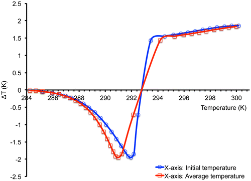
Figures 1 and 2 show plots of adiabatic temperature change, ΔT, versus initial and average temperature in gadolinium and Ni₅₁Mn_33.4In_15.6, respectively. For calculating average temperature, the initial temperature is added to the half of adiabatic temperature change at that initial temperature:(5) $$T_{\text{avg}}=T_i+{\left\{\frac{\mathrm{\Delta }{T}_{\text{ad}}}{2}\right\}}_{T_i}$$(5)

Figure 1. A comparison of gadolinium adiabatic temperature change as a function of initial temperature and average temperature with 2T applied field near the Curie temperature.

The computed areas under these two curves are different.

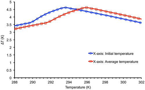
Figure 2. A comparison of Ni₅₁Mn_33.4In_15.6 adiabatic temperature change as a function of initial temperature and average temperature with 2T applied field near the Curie temperature.

The computed areas under these two curves are different.

In Figure 1, the adiabatic temperature change curve for gadolinium as a function of average temperature, ${\{\mathrm{\Delta }{T}_{\text{ad}}\}}_{T_{\text{avg}}}$, shows higher ΔT in temperature range above the Curie temperature and lower temperature change under the Curie temperature, compared to the adiabatic temperature change curve as a function of initial temperature, ${\{\mathrm{\Delta }{T}_{\text{ad}}\}}_{T_i}$.

In Figure 2 for Ni₅₁Mn_33.4In_15.6 Heusler alloy, in the inverse magnetocaloric region, the curve as a function of average temperature tends toward lower temperatures and in the conventional region tends toward higher temperatures compared to plotting the curve versus initial temperature. It should be noticed that in Figures 1 and 2 the differences between the curves (initial temperature and average temperature) are not simply a linear shift, but produces different areas under the curves.

The CF amount for gadolinium when ΔT_ad is plotted as a function of initial temperature is computed to be 58 K² for the temperature range of 14 K (288–302 K). Work by Griffel, Skochdopole, and Spedding (1954) reports an average specific heat capacity c_p − avg (within temperature range of 288–302 K) of gadolinium to be 0.28 J g⁻¹ K⁻¹. Hence, the COP is computed to be 116/W using Equation 4 for m = 100 g. In comparison, the calculation of COP at the Curie temperature, independent of CF, results to COP = 129/W, where m = 100 g, ΔT_ad = 4.62 K, and c_p = 0.285 at the Curie temperature. These results show that for our measurements on gadolinium, using CF in calculating COP, produces a 10% correction.

Furthermore, a CF value of 59 K² was computed from ΔT_ad plot as a function of average temperature, which shows 1.7% difference compared to the initial temperature for gadolinium. These results show that plotting ΔT_ad as a function of average temperature gives a different value for CF, compared to plotting ΔT_ad as a function of initial temperature. Plotting ΔT_ad versus average temperature emphasizes the reversibility of the MCE. For calculating the actual COP, the CF for average temperature should be used.

5. Conclusion

In this research, the adiabatic temperature change of gadolinium and Ni₅₁Mn_33.4In_15.6 Heusler alloy has been studied. The CF is defined as the area under the adiabatic temperature change versus ambient temperature curve. The CF gives a more representative measure of cooling performance in magnetic refrigeration. The relation between CF and COP has been presented. It has been shown that using average temperature in calculating the adiabatic temperature change results in a different, and more realistic, value for CF compared to the initial temperature.

Cover image

Source: Author.

Acknowledgments

We would like to thank Drs. Francis Johnson and Min Zou from GE Global Research for supplying the test sample and for useful discussions. We also would like to thank Professor Ekkes Brück for his comments on this work.

Additional information

Funding

Funding. This work was supported by the US Department of Energy and G.E. Global Research under award number DE-EE0003839.

Notes on contributors

Mohammadreza Ghahremani

Mohammadreza Ghahremani received his MSc degree in Computer Engineering from Sharif University of Technology in 1999 and PhD degree in Computer Engineering from the George Washington University in 2013. He was a research assistant at GWU from 2011 to 2013, where he conducted research in the area of magnetic refrigeration systems and magnetocaloric materials in collaboration with GE Global research. His research objective was to design and build an advanced magnetocaloric temperature change test system.

He is currently a postdoctoral research fellow in the Institute for Magnetics Research (IMR) at the George Washington University, where his research fields are magnetic refrigeration and energy efficient cooling systems.

References

- Bouchard, J., Nesreddine, H., & Galanis, N. (2009). Model of a porous regenerator used for magnetic refrigeration at room temperature. International Journal of Heat and Mass Transfer, 52, 1223–1229.10.1016/j.ijheatmasstransfer.2008.08.031
- Ghahremani, M., Jin, Y., Bennett, L. H., & Della Torre, E., ElBidweihy, H., & Gu, S. (2012). Design and instrumentation of an advanced magnetocaloric direct temperature measurement system. IEEE Transactions on Magnetics, 48, 3999–4002.
- Ghahremani, M., Seyoum, H. M., ElBidweihy, H., Della Torre, E., & Bennett, L. H. (2012). Adiabatic magnetocaloric temperature change in polycrystalline gadolinium—A new approach highlighting reversibility. AIP Advances, 2, 32149–32156.10.1063/1.4748131
- Griffel, M., Skochdopole, R. E., & Spedding, F. H. (1954). The heat capacity of Gadolinium from 15 to 355°K. Physical Review, 93, 657–661.10.1103/PhysRev.93.657
- Gschneidner, Jr., K. A., & Pecharsky, V. K. (2000). Magnetocaloric materials. Annual Review of Materials Science, 30, 387–429.10.1146/annurev.matsci.30.1.387
- Hu, J. C., & Xiao, J. H. (1995). New method for analysis of active magnetic regenerator in magnetic refrigeration at room temperature.. Cryogenics, 35, 101–104.10.1016/0011-2275(95)92877-U
- Jeppesen, S., Linderoth, S., Pryds, N., Kuhn, L. T., & Jensen, J. B. (2008). Indirect measurement of the magnetocaloric effect using a novel differential scanning calorimeter with magnetic field. Review of Scientific Instruments, 79, 83901–83906.10.1063/1.2957611
- Liu, J., Gottschall, T., Skokov, K. P., Moore, J. D., & Gutfleisch, O. (2012). Giant magnetocaloric effect driven by structural transitions. Nature Materials, 11, 620–626.10.1038/nmat3334
- Lucia, U. (2008). General approach to obtain the magnetic refrigeretion ideal coefficient of performance COP. Physica A: Statistical Mechanics and its Applications, 387, 3477–3479.10.1016/j.physa.2008.02.026
- Shir, F., Yanik, L., Bennett, L. H., Della Torre, E., & Shull, R. D. (2003). Room temperature active regenerative magnetic refrigeration: Magnetic nanocomposites. Journal of Applied Physics, 93, 8295–8297.10.1063/1.1556258
- Warburg, E. (1881). Magnetische untersuchungen [Magnetic investigations]. Annalen der Physik, 249, 141–164.10.1002/(ISSN)1521-3889
- Yu, B. F., Gao, Q., Zhang, B., Meng, X. Z., & Chen, Z. (2003). Review on research of room temperature magnetic refrigeration. International Journal of Refrigeration, 26, 622–636.10.1016/S0140-7007(03)00048-3