Impact of Real Shocks on Business Cycles in selected Sub-Saharan African Countries

Abstract

This study examines business cycle fluctuations in selected Sub-Saharan African (SSA) countries. The study measures the impact of selected real shocks, namely: terms of trade shocks, commodity price shocks, and government spending shocks, on macroeconomic fluctuations in SSA. The impact of the selected shocks was measured by the Bayesian Panel Vector Autoregression (BPVAR) technique. It was ascertained from the results that real (i.e. productivity) shocks drive business cycles (macroeconomic fluctuations) in SSA countries which support theoretical inclination. Furthermore, from the empirical analysis, terms of trade shocks possess the highest positive impact on business cycles. At the same time, government expenditure has the highest negative impact on business cycle among the three selected real shocks across the SSA region. Thus, the study recommends that government institutions in SSA should embark on sound fiscal policy plan along with monetary policy to stabilise the economy during recessions and expansions. The study highlights the need for diversification of the export base of SSA countries to mitigate terms of trade losses usually occasioned by unfavourable commodity price shocks.

Keywords:

• Bayesian panel VAR
• macroeconomic fluctuations
• real business cycle
• real shocks
• Sub-Saharan Africa

JEL classification:

• C11
• C33
• E19
• F44

PUBLIC INTEREST STATEMENT

Business cycles are influenced uniquely in developing countries and these influences are spurred by political and economic crises. These crises induce macroeconomic fluctuations which are evidenced by the wave of shock triggered by either domestic or external factors. The global economic and financial downturn experienced in 2007/2008 which began as the sub-prime mortgage turmoil in the United States in 2007 turned into financial crisis that induced an economic recession in developed economies by 2008. This further induced a development crisis in Africa from 2009. The unprecedented nature of the crisis resulted in a continuous and large downward trend of major macroeconomic indicators in Africa for which the economy of most African countries declined as an aftermath of the global financial crisis. This study empirically investigates the issues pertinent to the drivers of business cycles in Africa.

1. Introduction

Economies strive to experience high and stable economic expansion devoid of macroeconomic fluctuations. This is often unachievable as proven by the recession phase of the business cycle. A recession is characterised by a decline in Gross Domestic Products (GDP) in two consecutive quarters. A period of recession may last for more than a few months, resulting in increased unemployment rate, fall in real income, reduction in productivity, and reduction in aggregate demand. Therefore, analysing business cycles is useful for a variety of reasons. Such insights could guide researchers in selecting principal indicators for economic activity, and provide a set of “regularities” which macroeconomists can use as a benchmark to examine the validity of numerical versions of theoretical models like the Real Business Cycle (Burns & Mitchell, 1947).

Business cycles are influenced uniquely in developing countries, and these influences are spurred by political and economic crises. These crises induce macroeconomic fluctuations which are evidenced by the wave of shock triggered by either domestic or external factors. The global economic and financial downturn experienced in 2007/2008, which began as the sub-prime mortgage turmoil in the United States in 2007 turned into a financial crisis that induced an economic recession in developed economies by 2008. This further caused a development crisis in Africa from 2009. The unprecedented nature of the crisis resulted in a continuous and large downward trend of major macroeconomic indicators in Africa for which the economy of most African countries declined as an aftermath of the global financial crisis (Adeleye, Osabuohien, Bowale, Matthew & Odutan, 2018). For instance, the economic growth of Nigeria, the largest economy in the continent, dipped from 6.3 percent in 2008 to 4.5 percent, 2.7 percent and 2.2 percent in 2012, 2015 and 2019, respectively (World Bank, 2020).

The scenario was the same in South Africa where economic growth declined from 3.2 percent in 2008 to 2.22 percent, 1.28 percent and 0.15 percent in 2012, 2015 and 2019, respectively; while the case is not different in Egypt, Morocco, Malawi and most of the African countries (World Bank, 2020). The percent of market capitalisation to Gross Domestic Products (GDP) declined in Nigeria from 23 percent in 2008 to 10.4 percent in 2015 and 9.8 percent in 2019. The downturn was also witnessed in Egypt, which nose-dived from 48 percent to 16 and 14 percent, respectively, during the same period (World Bank, 2020). Therefore, an understanding of the causes and consequences of these fluctuations has motivated individuals, policymakers, and researchers towards business cycle research.

The 2016/2017 recession observed in Nigeria, increased the level of awareness on the need to study business cycles more extensively within the African continent. In the second quarter of 2016, Nigeria’s GDP declined by −2.06 percent in real terms, following an initial decline in the first quarter of the same year of −0.36 percent (National Bureau Statistics, 2016). According to the NBS, Nigeria entered into the recession phase of the business cycle by the second quarter of 2016. The business cycle fluctuation experienced by African countries motivates this study to attempt to apply the RBC theory in examining the effects of real shocks in driving macro-economic fluctuations in Nigeria and other selected Sub-Saharan countries. Thus, increasing the literature on business cycle research in developing economies.

Given the existing literature on business cycles, in both developed and developing countries, this study is conducted with the view of exploring the sources of the shocks that influence business cycle fluctuations, in the spirit of the real business cycle theory in Africa. Macroeconomic variables in many African economies have been highly unstable for over a decade (Combes et al., 2014). Towards the goal of reducing these large fluctuations displayed by the cyclical components of macroeconomic variables in the region. The study examines the effect of real shocks on the business cycles in Africa. The focus of this study on the African continent increases the quality, as well as the quantity of literature on business cycle research in the region but also as emerging market economies, are gaining traction globally, it is resourceful to investors and policymakers. The outcome of this study is resourceful to policymakers and investors because the knowledge gained will indicate the importance and significance of priority sectors to focus policies and invest funds that will drive economic growth as well as business cycles in African countries.

The sources of these shocks are, however, pivotal in understanding the nature of these macroeconomic fluctuations. Alege (2008) examined the role of sources of these shocks (real shocks, money supply shocks and external trade shocks) in driving macro-economic fluctuations in Nigeria. Establishing that short-run behaviour of macroeconomic time series was influenced by real shocks, while long-run behaviour, on the other hand, was determined by nominal shocks. This research is thus premised on the investigation of macro-economic fluctuations in Sub-Saharan Africa by determining how much these fluctuations are influenced by real shocks, in the spirit of the real business cycle theory as a gap identified in the literature. Hence, the study extends Alege (2008) study to test out the real business cycle theory in SSA. The rest of the study consist of section two with the insights from literature, section three with the theoretical framework guiding the study, section four with the empirical analysis while section five contains the conclusion and recommendation based on the study.

2. Insights from the literature

This section reviews relevant literature which explains the relationship between real, nominal shocks and business cycles. It focuses on an empirical review of relevant literature. The empirical review shows other research work findings in sub-Saharan Africa and selected African countries. Olaniran et al. (2017) examined the dynamic interaction among business cycle, macroeconomic variables and economic growth in Nigeria between 1986 and 2014. The study employed the vector autoregression technique (VAR) to investigate the business cycle effect on economic growth and its interaction with government expenditure and money supply in Nigeria during the study period. Quarterly time series data between 1986 and 2014 was used for the study. They found that business cycle affected growth and the performance of macroeconomic variables in the study period, although its effect lacked persistence throughout the study period.

Patroba and Raputsoane (2016) investigated how far permanent and transitory productivity shocks can account for the dynamics observed in the South African business cycle (1946–2014) using Bayesian VAR techniques with annual South African data on output growth, consumption growth, investment growth and the trade balance to output ratio. By estimating a standard small open economy real business cycle model and its financial frictions augmented counterpart, which shows that permanent productivity shocks are more critical than transitory ones in explaining this country’s business cycle fluctuation. The authors found that financial frictions such as country risk premium shocks help to explain the fluctuations in investment and the trade balance to output ratio.

Alege (2009) employed small business cycle model in line with the Dynamic Stochastic General Equilibrium (DSGE)-VAR techniques to investigate the sources of business cycle fluctuations in Nigeria and used the model for policy analysis. The study employed annual and quarterly data covering periods from 1970 to 2004. This study highlighted the policy implications of monetary supply, technology and export supply shocks on some macroeconomic aggregates such as namely consumption, labour, price level, deposits, loans, interest rate, wage rate, money supply, export, and aggregate output and capital stock. The study adopts the models of Nason and Cogley (1994) and Schorfheide (2000), but the author incorporates the export sector into the model to assess the transmission channel of terms of trade. The results obtained showed that the business cycle exists in Nigeria, and it is driven by both real and nominal shocks. Specifically, productivity shock, money supply growth shock and export supply growth shock contributed in the significantly in explaining business cycle in the country.

Sissoko and Dibooglu (2006) examined the sources of business cycles in sub- Saharan Africa (SSA) countries with particular attention to the exchange rate system. The study covered 30 sub-Saharan African countries from both the CFA and the non-CFA zone from the period 1960 to 2000. A small open economy of aggregate demand and supply model was adopted to reflect exogenous capital mobility. The essence of the model was to allow the capture of five identified economic disturbances, namely: terms of trade shocks, aggregate supply shocks, trade balance shocks, money supply shocks and real demand shocks.

In characterising the impact of the identified economic disturbances, terms of trade shocks influence macroeconomic fluctuations in both the CFA and the non-CFA countries alike. In contrast, domestic shocks play a limited role in the variation of the terms of trade. Business cycles are majorly driven by supply shocks, as they dominate changes in output at both short and long-term forecasting horizons. Real demand shocks, on the other hand, play a limited role in the CFA countries. The trade balance or balance of payment shocks do not account for significant influence in changes in output movements in CFA countries. Whereas, external shocks such as terms of trade disturbances seem to matter to macroeconomic fluctuations in output. Further analysis shows evidence that the impacts of terms of trade shocks on output can be attributed to the exchange rate system in the CFA countries (Sissoko & Dibooglu, 2006).

Real exchange rate fluctuations in the non-CFA countries are mostly caused by disturbances to both terms of trade and the balance of payment, otherwise known as the trade balance. However, monetary shocks affect real exchange rate movements in the non-CFA countries, indicating the impact of the flexible exchange rates system that is present in the region. Monetary shocks are also the main source of fluctuations in the price level in Sub-Saharan Africa. However, terms of trade, real demand and supply shocks also play a significant role in these countries. As for the role of the exchange rate system, there does not appear to be a major difference in the source of the price level movements in the CFA versus the non-CFA countries (Sissoko & Dibooglu, 2006).

Literature examination brings to the fore the test of the real business cycle theory in Sub Saharan Africa region and a comparison of the impact of some identified shocks which include terms of trade shocks, commodity price shocks, and government spending shocks on business cycle in the SSA region have not been addressed and discussed. Hence, this study contributes and fills this observed gap by testing the hypothesis of the existence of the real shocks as a determinant of business cycles.

3. Theoretical framework and methodology

3.1. The real business cycle theory

The emphasis on the role of real shocks (particularly technological shocks) in driving business fluctuations as first presented by Kydland and Prescott (1982), is the idea behind the real business cycle (RBC) theory. Prescott (1986) computes total factor productivity (TFP) and treats it as a measure of exogenous technology shocks. The other shocks include but are not limited to monetary, fiscal and oil price shocks. However, Prescott presents an argument that technology shocks account for more than half the macroeconomic fluctuations. The RBC theory views recessions and booms as efficient responses to exogenous changes in the real economic environment. Business cycles do not represent a failure of markets to clear but rather reflect, possibly, most efficient operations of the economy, given the structure of the economy and the rationality of the economic agents. The construction of the model is based on rational expectations and expected utility maximisation. The theory holds the view that the level of output in the economy at any point maximises the expected utility of the economy-wide agents.

3.2. The structure of the RBC model

There is a consensus that booms are preferred to recessions. Given that economic agents make optimal choices towards prosperity, fluctuations are then necessarily caused by factors outside the decision-making process. The question then remains what exogenous factors influence the decision making by economic agents. Kydland and Prescott (1982) pioneered a new perspective of macroeconomics by building a theoretical framework to account for the observed fluctuations. They stated the exogenous factor responsible for these fluctuations to be technology shocks, that is, fluctuations in the productivity level that shifted aggregate output trend up and down. These fluctuations are said to be real because they are direct changes in the effectiveness of capital and labour. This influences the decisions of workers and firms, who in turn change their consumption and investment pattern; thus, resulting in a change in aggregate output level.

The Real Business Cycle (RBC) theory relies on the neoclassical concept of rational expectations and expected utility maximisation. Therefore, it is imperative to understand the central assumption of the theory: individuals and firms respond to economic events optimally at all times. In a recession preceded by an undesirable productivity shock which introduces constraints, economic agents make decisions that would maximise their expected utility and achieve the best output level. This means that the low output level experienced in recessions are a result of the optimal choices of economic agents to maximise expected utility. This is to say that recessions and booms are responses to exogenous innovations in the real economic environment.

The RBC theory possesses two underlying principles. First, money holds little importance in business cycles. The theory holds that monetary shocks are not significant in explaining aggregate output fluctuations. Second, business cycles result from rational economic agents responding to real shocks optimally. These real shocks are assumed to result from mostly fluctuations in productivity growth (technological progress). A simple RBC model includes only the household and firms, without the government and external sectors. The model is, however, based on the standard neoclassical growth model where the economy is characterised by a large number of identical infinitely lived households with similar preferences over consumption goods and in which steady-state growth is zero. According to King and Rebelo (1999) and Aleksander (2016), considering a theoretical economy, a representative household maximises the following utility function:

(3.1) $U=\sum _{i=o}^{\mathrm{\infty }}{\beta }^{t}u\left(C_t,L_t\right),0<\beta <1$(3.1)

Where $C_t$ denotes the household’s consumption at time t. $L_t$ denotes leisure during time period t. $\beta$ refers to a discount factor that shows the individuals preference for present over future consumption-leisure bundles. There is a strict assumption that the function $u\left(C_t,L_t\right)$must be increasing, concave and satisfy inada conditions. This ensures that an individual in the model always consumes a positive quantity of consumption and leisure bundles.

All individuals in the economy have time as their fundamental endowment, which is shared between working hours ($N_t)$ and leisure ($L_t$). The total amount of time in each period given to an individual possesses the following resource constraint:

(3.2) $N_t+L_t=1$(3.2)

However, for the firm’s behaviour, given the assumption that there is only one homogenous good being produced, total product/output is assumed to be dependent on a production function that combines labour ($N_t)$ and capital $\left(K_t\right)$ inputs. The function is given as:

(3.3) $Y_t=A_{t}F\left(K_t,N_t{X}_t\right)$(3.3)

In the above function, $A_t$ is a random productivity shock factor the represents total output not explained by the amount of inputs utilised in the production process. $X_t$ represents the deterministic component of productivity which expands at a constant rate, expressed as:

(3.4) $X_{t+1}=\gamma X_t,\gamma >1$(3.4)

The stock of capital $K_t$ changes over time and depreciates at a constant rate $\left(\delta \right)$ this represents the definition of Investment and is expressed as:

(3.5) $K_{t+1}=I_t+\left(1-\delta \right)K_t$(3.5)

Total output produced in the economy can be utilised for either consumption $C_t$ or investment $I_t$ purposes. Therefore, the following resource constraint on the economy is expressed as:

(3.6) $Y_t=C_t+I_t$(3.6)

The need to add an assumption to the utility function arises to achieve the desired steady-state to transform the economy. The utility function is then presented as in King and Rebelo (1999):

(3.7) $u\left(C_t,L_t\right)=\frac{1}{1-\sigma }{C}_t^{1-\sigma }V\left(L_t\right)$(3.7)

The above equation compensates for the income and substitutability effects of wage changes in supply. This enables the transformation of the economy as all variables are presented in efficiency units by scaling the variables with the initial level of the deterministic component. The transformed utility function is then expressed as:

(3.8) $\sum _{i=o}^{\mathrm{\infty }}{\left({\beta }^{\ast }\right)}^{t}u\left(C_t,L_t\right)$(3.8)

Where ${\beta }^{\ast }=b{\gamma }^{1-\sigma }$ is a modified discount factor that satisfies the condition $0<\beta <1$. The transformed utility function is then maximised with the following the resource constraints:

(3.9) $\mathrm{L}\mathrm{a}\mathrm{b}\mathrm{o}\mathrm{u}\mathrm{r}:N_t=1-L_t$(3.9)

The production function:

(3.10) $Y_t=A_{t}F\left(K_t,N_t\right)$(3.10)

The Resource Constraint:

(3.11) $Y_t=C_t+I_t$(3.11)

The Law of Motion of Capital:

(3.12) $\gamma K_{t+1}=I_t+\left(1-\delta \right)K_t$(3.12)

To obtain the optimal path for consumption, $C_t$, leisure $L_t$, labour $N_t$ and capital stock $K_t$, the transformed utility function is subjected to the relevant constraint. This is achieved using the Lagrangian multiplier approach:

(3.13) $\mathcal{L}=\sum _{i=o}^{\mathrm{\infty }}{\left({\beta }^{\ast }\right)}^{t}u\left(C_t,L_t\right)+\sum _{t=0}^{\mathrm{\infty }}{\beta }^t{\lambda }_t(A_{t}F\left(K_t,N_t\right)+\left(1-\delta \right)K_t-C_t-\gamma K_{t+1}+\sum _{t=0}^{\mathrm{\infty }}{\beta }^t{\omega }_t\left(1-L_t-N_t\right)$(3.13)

Hence, the first-order conditions (FOC) are:

$C_t:D_{1}u\left(C_t,L_t\right)={\lambda }_t$

$L_t:D_{2}u\left(C_t,L_t\right)={\omega }_t$

$N_t:{\lambda }_t{A}_t{D}_{2}F\left(K_t,N_t\right)={\omega }_t$

$K_{t+1}:\beta {\lambda }_{t+1}\left[A_{t+1}{D}_{1}F\left(K_{t+1},N_{t+1}\right)+1-\delta \right]=\gamma {\lambda }_t$

The notation $D_{i}u\left(C,L\right)$is used to denote the partial derivative of the function $u\left(C_t,L_t\right)$ for the ith term. Consumption, labour and capital are independent over time, and the optimal decision are taken in consideration of the resource constraint of the economy.

3.3. Method of data analysis

This thesis establishes an argument that real shocks are drivers of business cycle fluctuations in Africa. This study holds the position that, these shocks can affect macroeconomic variables in any country. Thus, a negative real shock to the economy can reduce total output and increase the unemployment rate, and vice versa. This study further examines the effects of real shocks on business cycles in African countries using the Bayesian Panel Vector Autoregressive (Bayesian PVAR) approach.

3.3.1. Model specification

The study adapts the model of Alege (2008), which expressed the determinants of the business cycle model for Nigeria as a function of the economic agents/actors/sectors in an economy and their interactions. For example, the economic agents include the household, firms, external sector and the government. The household is expected to consume, and the government is expected to expend and regulate prices. These roles are captured in the economy by household consumption, government expenditure and commodity price, respectively. These and more are expressed in the empirical model. However, this study adopts a partial equilibrium framework as against a general equilibrium framework and hence, drops some monetary variables and adds the terms of trade variable, given that the study focuses on testing the real business cycle theory strictly. The empirical model is specified in its implicit form initially as follows:

RGDP _it = f (GFI_it, IMP_it, EXPT_it, TOT_it,COMP_it, GEXP_it, HCON_it) (3.14)

Where:

RGDP: Real Gross Domestic Product

GFI: Gross Fixed Investment

IMP: Total Import

EXPT: Total Export

TOT: Terms of Trade

COMP: Commodity Price

GEXP: Government Expenditure

HCON: Household Consumption

i: represents individual countries

t: represents the period

Assuming the existence of a non-linear relationship between the dependent variable and the explanatory variables, the model can be written explicitly as follows:

RGDP_it = A. GFI_it^α1. IMP_it ^α2. EXPT_it ^α3. TOT_it ^α4.COMP_it ^α5GEXP_it ^α6. HCON_it ^α7.e_it (3.15)

To carry out the various econometric tests, the model is then linearised by taking the double log of both sides, which are the dependent and the independent variables and is represented as:

lrgdp_it = α₀ + α₁lgfi_it + α₂limp_it+ α₃lexpt_it + α₄ltot_it + α₅lcomp_it + α₆lgexp_it + α₇lhcon_it + e_it (3.16)

From business cycle literature, the gross domestic product (GDP) is an important indicator as it is used to measure the total level of economic activities in any economy. The trend of the GDP serves as an indicator for an economy heading towards economic expansion or recession. This study, however, utilises the real gross domestic product (RGDP) as it helps to capture the real effects of shocks to the economy, as the RGDP considers the price level and inflation.

Household consumption and government expenditure are included in this study, as they are components of GDP. This is based on the fact that household consumption is the total amount of goods and services bought and consumed by the private or household sector. This is important, as it is an indicator of business cycle fluctuations. It reflects the decision of individual agents in the economy, at different periods of the business cycle. During periods of economic recession, there tends to be a decrease in consumption levels, while during an expansion, consumption tends to increase.

Government expenditure is used to capture fiscal policies. It refers to the total amount of goods and services purchased by the government. Figures from the stylised facts established that government expenditure is strongly pro-cyclical among the selected African countries. This then requires an explanation of how shocks can impact the decisions of the government. Gross fixed Investment is included in the model as it is a significant variable in the business cycle literature. As investment spurs more investment in countries with large markets, the economy grows, leading to economic expansion.

Total imports and exports are included in the model as trade is essential. Total imports refer to the total goods and services purchased by residents of a country. This includes citizens, businesses, and the government. Total exports; on the other hand, refer to the total amount of goods and services sold to other countries. The participation of a large number of African countries in international trade for foreign exchange earnings reflects on trade balances. Therefore, a negative balance of trade reduces the external reserves and increases debt portfolio, which could lead to an economic downturn or recession.

The notable contribution to the existing empirical model is the commodity price, government expenditure and terms of trade, which are proxies for productivity shocks or otherwise called real shocks. This study, therefore, examines how shocks to real macroeconomic variables affect business cycles in the region.

3.4. Technique of estimation a. The Bayesian panel vector autoregressive model

To examine the effects of real shocks on business cycles in Africa, the econometric method of Bayesian PVAR is utilised. This technique of estimation makes use of Bayes rules on the standard PVAR models to overcome some of the limitations of the unrestricted VAR method. Panel VAR models have gained popularity in the field of macroeconomic analysis in studying transmission shocks across countries (Ballabringa et al., 2000). Canova and Ciccarelli (2013) also utilised panel VAR models in the realm of business cycles, as they examined the cross-sectional dynamics of Mediterranean business cycles. Cyclical indicators of leading nature, as well as forecasts, can be easily constructed as well as forecasts using panel VARs. Also, technological advancement has aided in estimating increasingly complex VAR models making it available for a variety of decision making and forecasting purposes.

Panel VARs have the same structure as VAR models, meaning that all variables are assumed to be endogenous and interdependent. However, the difference is the addition of a cross-sectional dimension which is a more suitable tool in addressing issues relating to transmission of shocks across countries. They are particularly suited to: (a) capture both static and dynamic interdependencies; (b) treat the links across units in an unrestricted fashion; (c) easily incorporate time variations in the coefficients and in the variance of the shocks; and (d) account for cross-sectional dynamic heterogeneities (Canova & Ciccarelli, 2013). Canova and Ciccarelli (2013) further emphasised that Panel VAR models have three distinctive features which are: 1. Lags of all endogenous variables of all units enter the model for unit i. This is called dynamic interdependence; 2. U_it are generally correlated across i. This feature is described as static interdependence; and 3. The intercept, slope and the variance of the shocks may be unit specific. This is referred to as cross-sectional heterogeneity.

For this study, the Bayesian approach is used in estimating the VAR models. The technique was popularised to literature by the works of Doan et al. (1984), Litterman (1986), and Sims and Zha (1998). This approach creates a suitable framework where one can allow both interdependencies and time variations in the coefficients. The Bayesian approach proffers a solution to the “overfitting” problem associated with the unrestricted VAR approach. Unlike the unrestricted VAR approach, the Bayesian VAR approach considers uncertainty in the population and therefore, it does not rely completely on the model parameters. This uncertainty is considered in the form of a prior probability distribution. This prior symbolises the degree of uncertainty in the value of the parameters and thus lowers the possibility of overfitting.

Bayesian VARs are known to allow some level of flexibility. The model utilises the prior knowledge and economic theory which improves the forecasting ability of the model. Bayesian VARs are preferred to produce better forecasts than unrestricted VARs, ARIMA or structural models (Canova, 1994). This is because the model allows interdependencies and some degree of information pooling across units with the same level of flexibility. Applying the Bayes rules to VAR models presents a probability distribution and a posterior distribution. This offers complete knowledge on the model parameters from data observation initially derived. Second, a prior distribution that shows the degree of uncertainty of the parameters before the data observation is also utilised. There are several prior distributions associated with Bayes theorem. These priors include: Minnesota or Litterman prior, hierarchical prior, diffuse prior, Normal-diffuse prior and normal conjugate prior.

The Minnesota type prior is adopted for the study. Prior specifications are essential in Bayesian analysis because it simplifies the posterior distribution. This prior transforms VAR estimates into a multivariate random walk model. According to Ejemeyovwi, Osabuohien and Bowale (2020) the Minnesota prior accounts for the non-stationarity observed among time series. Given the high dependence of the intertemporal variables, the prior mean of the VAR coefficients on the first own lag is one, while for the other coefficient is equal to zero. The covariance matrix is diagonal, and coefficients of higher-order lags are close to zero (i.e. the prior variance decreases with an increase in lag length).

Since the variations on variables in VARs are accounted for by own lags, coefficients other than the dependent one are assigned smaller relative variance. Finally, the variance-covariance matrix of the error term is assumed to be fixed and known. The panel VAR model presented in this study is adapted from the works of Gavin and Theodorou (1984); Alege and Osabuohien (2009), which is of the form:

(3.17) $Y_{it}=A_{it}+B_i\left(L\right)Y_{it-1}+{\mu }_{it}$(3.17)

Where $Y_{it}$ $=$ $\left[\begin{array}{c}lrgd{p}_{it}\\ lgf{i}_{it}\\ lim{p}_{it}\\ lexp{t}_{it}\\ lto{t}_{it}\\ lcom{p}_{it}\\ lgex{p}_{it}\\ lhco{n}_{it}\end{array}\right]$; $A_i$ $=\left[\begin{array}{c}{\beta }_{rgdp}\\ {\beta }_{gfi}\\ {\beta }_{imp}\\ {\beta }_{expt}\\ {\beta }_{tot}\\ {\beta }_{comp}\\ {\beta }_{gexp}\\ {\beta }_{hcon}\end{array}\right]$; ${\mu }_{it}$ $=\left[\begin{array}{c}{\mu }_{rgdp}\\ {\mu }_{gfi}\\ {\mu }_{imp}\\ {\mu }_{expt}\\ {\mu }_{tot}\\ {\mu }_{comp}\\ {\mu }_{gexp}\\ {\mu }_{hcon}\end{array}\right]$ (3.18)

$Y_{it}$ presents a vector of endogenous variables as defined in equation (4.14) for time, t $=$ 1, … , 15 and individual countries, i $=$ 1 to 15. The vector $Y_{it}$ consist of the logarithms of the specified variables (RGDP, GFI, IMP, EXPT, TOT, COMP, GEXP, HCON), as defined in equation (4.14). $A_i$ is a (8$\times$1) vector of the individual country’s intercept parameters.$B_i(L$) is a (8$\times 8$) matrix of lag polynomials with L identifying as the lag operator. The elements are typically presented with the form: $\sum _{\mathrm{j}=1}^{\mathrm{n}}{\alpha }_{\mathrm{i}\mathrm{x}\mathrm{y}\mathrm{j}}{\mathrm{L}}^{\mathrm{j}}$, where n is the number of lags in the model, x and y are indices over the endogenous variables. The residual ${\mu }_{it}$ is a (8$\times$1) vector of error terms with variance ${\sigma }_i^2$ for each country, indicating a normal distribution. The residuals are assumed to be contemporaneously correlated across equations, but serially uncorrelated, for each country. To estimate the panel vector autoregressive model, the equation for an individual country can be written as follows:

(3.19) $\begin{array}{rl}& Y_{it}={\beta }_{yi}+\sum _{j=1}^n{\alpha }_{1yyj}{Y}_{i-j}+\sum _{j=1}^n{\alpha }_{1ygfij}lgf{i}_{i-j}+\sum _{j=1}^n{\alpha }_{1yimpj}lim{p}_{i-j}+\\ & \sum _{j=1}^n{\alpha }_{1yexptj}lexp{t}_{i-j}+\sum _{j=1}^n{\alpha }_{1ytotj}lto{t}_{i-j}+\sum _{j=1}^n{\alpha }_{1ygexpj}lgex{p}_{i-j}+\\ & \sum _{j=1}^n{\alpha }_{1ycompj}lcom{p}_{i-j}+\sum _{j=1}^n{\alpha }_{1yhconj}lhco{n}_{i-j}+{\mu }_{it}\end{array}$(3.19)

Equation (4.19) represents the VAR model for an individual country for lrgdp ($Y_{it}$). The other endogenous variables (lgfi, limp, lexpt, ltot, lgexp, lcomp, lhcon) have similar equations, as shown in equation (4.19) above. The panel vector autoregressive equations for the 15 individual countries considered for the study are derived by stacking the system of equations in equation (5.18) for each country. This creates a more extensive system of equations that is then estimated using the Bayesian PVAR approach.

The study proposes to investigate the effects of real shocks on business cycle fluctuations in Africa. We introduce commodity price, government spending and terms of trade shocks as proxies for productivity shocks, as sources of real business cycle fluctuations in Africa. We introduce these shocks to six macroeconomic variables: real GDP, Total Import, Total Export, Investment, Household Consumption and Government expenditure across the selected African countries.

Utilising Minnesota prior to estimate the Bayesian PVAR, the Impulse Response Function (IRF) and Variance Decomposition (VD) are generated for the imposed shocks included in the model. The IRF and VD are used to estimate the impact of these shocks across the selected countries for this study over 15 years.

Impulse response functions are essential in studying the interactions between variables in the vector autoregressive model. They represent the reactions of variables to shocks in the model. This technique is relevant to achieving the objectives of this study. The variance decomposition is useful in evaluating how shocks reverberate through the dynamic system (i.e. to assess the pass-through of external shocks to each economic variable). That is the variance decomposition techniques enables us to estimate the amount of variation in the system is caused by a shock to one variable.

3.5. Data sources and measurements

This study employs annual time series data covering various macroeconomic variables that are required to determine the effect of real shocks on business cycle fluctuations in Africa. The data was sourced from annual publications by World Bank (2020. The variables utilised include Real Gross Domestic Products, Gross Fixed Investment, Total Import, Total Export, Terms of Trade, Commodity Price, Government Expenditure, and Household Consumption. The scope of this study covers fifteen countries over 15 years, 2001 to 2015. The choice of the period, as well as cross-section, is considered to be sufficient enough in analysing the dynamic nature of the variables considered and their effect on the business cycles in Africa. The cross-section countries selected for this study are from Sub-Saharan Africa. Given the economic and political peculiarities of Sub-Saharan Africa, the study focuses on this region. Therefore countries chosen for this study include: Botswana, Burundi, Kenya, Liberia, Malawi, Mauritius, Mozambique, Namibia, Nigeria, Rwanda, Sierra Leone, South Africa, Swaziland, Tanzania and Uganda. The scope of the study was also influenced by data unavailability among African countries.

4. Estimation results and discussion

This section presents the empirical coefficients for the impact of real shocks on macroeconomic fluctuations in Sub-Saharan Africa. The Bayesian PVAR model, as specified in the previous section using the Minnesota prior is used to achieve this objective. The impulse response function (IRF) and variance decomposition (VD) are presented in Tables 1 and 2, respectively (see Appendix). These are used in discussing the impact of real shocks on business cycles. This is done in furtherance of the study as it leads to the conclusion and implication of findings in the next section.

Table 1. Impulse response of the macroeconomic variables to real shocks in Africa

Accumulated Response of LGDP
Period	LCOMP	LGEXP	LTOT
1	0.000000	0.000000	0.000000
3	−0.007049	−0.005932	0.004791
5	−0.015775	−0.018501	0.009946
7	−0.024745	−0.035376	0.015122
9	−0.033951	−0.055099	0.020549
10	−0.038642	−0.065743	0.023355
Accumulated Response of LHCON
Period	LCOMP	LGEXP	LTOT
1	−0.009118	−0.017869	0.000000
3	−0.019392	−0.052007	0.010500
5	−0.029824	−0.088271	0.023405
7	−0.039399	−0.123938	0.036158
9	−0.048534	−0.158385	0.048180
10	−0.053011	−0.175111	0.053836
Accumulated Response OF LGFI
Period	LCOMP	LGEXP	LTOT
1	−0.017326	−0.027622	0.000000
3	−0.054286	−0.049207	0.032408
5	−0.080135	−0.049538	0.071345
7	−0.102314	−0.044112	0.105867
9	−0.121895	−0.040034	0.132969
10	−0.130936	−0.039438	0.143920
Accumulated Response of LGEXP
Period	LCOMP	LGEXP	LTOT
1	−0.016288	0.148750	0.000000
3	−0.044905	0.312595	0.003815
5	−0.069690	0.414836	0.005021
7	−0.089944	0.478062	0.007030
9	−0.107172	0.516214	0.010908
10	−0.114968	0.528588	0.013401
Accumulated Response of LIMP
Period	LCOMP	LGEXP	LTOT
1	0.002288	−0.004720	0.000000
3	0.004918	0.006783	0.024310
5	0.006843	0.019131	0.059985
7	0.009320	0.028358	0.094503
9	0.011682	0.033519	0.124361
10	0.012673	0.034584	0.137343
Accumulated Response of LEXPT
Period	LCOMP	LGEXP	LTOT
1	0.028873	0.000000	0.000000
3	0.071347	−0.012146	−0.001048
5	0.105204	−0.025971	0.003466
7	0.131922	−0.039949	0.010333
9	0.152511	−0.054134	0.018633
10	0.160831	−0.061382	0.023085

Source: Authors’ compilation using E-views 9.0

Table 2. Variance decomposition of real shocks in Africa

	Variance Decomposition of LGDP
Period	S.E	COMP	GEXP	TOT
1	0.047533	0.000000	0.000000	0.000000
2	0.064552	0.202282	0.090836	0.111380
3	0.078180	0.419142	0.321996	0.189638
4	0.089816	0.550694	0.636018	0.228198
5	0.100178	0.634631	0.991907	0.247936
	Variance Decomposition of LHCON
Period	S.E	COMP	GEXP	TOT
1	0.081216	1.260322	4.840829	0.000000
2	0.098885	1.025736	5.838840	0.225077
3	0.114038	1.060279	6.958411	0.428712
4	0.125506	1.056714	7.820462	0.617279
5	0.135157	1.052895	8.553333	0.761010
	Variance Decomposition of LGFI
Period	S.E	COMP	GEXP	TOT
1	0.178564	0.941460	2.392819	0.000000
2	0.222752	1.532888	1.996354	0.401198
3	0.247666	1.631807	1.683774	0.870429
4	0.263994	1.695939	1.485630	1.313785
5	0.275773	1.756163	1.363579	1.698836
	Variance Decomposition of LGEXP
Period	S.E	COMP	GEXP	TOT
1	0.162174	1.008765	84.12945	0.000000
2	0.195059	1.171581	79.56906	0.013619
3	0.216791	1.438968	75.93506	0.016065
4	0.231862	1.576911	72.46885	0.015048
5	0.243245	1.663763	69.27469	0.014047
	Variance Decomposition of LIMP
Period	S.E	COMP	GEXP	TOT
1	0.140462	0.026542	0.112921	0.000000
2	0.176299	0.031336	0.174652	0.274729
3	0.199857	0.025029	0.221462	0.782323
4	0.216522	0.022829	0.277354	1.323774
5	0.229199	0.022617	0.313789	1.806492
	Variance Decomposition of LEXPT
Period	S.E	COMP	GEXP	TOT
1	0.184411	2.451309	0.000000	0.000000
2	0.230688	2.510141	0.065561	0.009607
3	0.266525	2.447234	0.103912	0.009269
4	0.293249	2.390225	0.141527	0.011810
5	0.314623	2.336759	0.171121	0.017214

Source: Author’s compilation using E-views 9.0

The results of the accumulated responses of the shock variables: Commodity Price (COMP), Government Spending (GEXP) and Terms of Trade (TOT) to major macroeconomic variables in Africa using some selected SSA countries are presented (Figure 1 and Table 1). The responses of selected macroeconomic variables to these three exogenous shocks were examined over ten horizons (years). In the first period, a one percent shock to commodity price, Government spending and terms of trade have no impact on real GDP. However, the impact of these shocks on real GDP was observed from in subsequent horizons. By the third period to be precise, shocks to commodity price and Government expenditure led to a negative impact of 0.70 percent and 0.59 percent on real GDP. At the same horizon, a one percent shock to terms of trade had a positive impact of 0.48 percent on real GDP. This trend was maintained throughout the horizons examined. Government spending exhibits the most substantial impact on GDP in the tenth period with 6.57 percent. From observing the impact of the exogenous shocks to private consumption, a one percent shock to commodity price and Government spending in the first period leads to a negative impact of −0.91 percent and −0.18 percent, respectively. In the same period, a one percent shock to terms of trade does not have an impact on private consumption levels. However, in the third period, a shock to terms of trade leads to a positive impact of 3.24 percent. The trend of the response of private consumption continues throughout the horizons considered for the study. Terms of trade, however, shows the largest impact on private consumption with 14.4 percent in the tenth period.

Figure 1. Impulse response of macroeconomic variables to real shocks

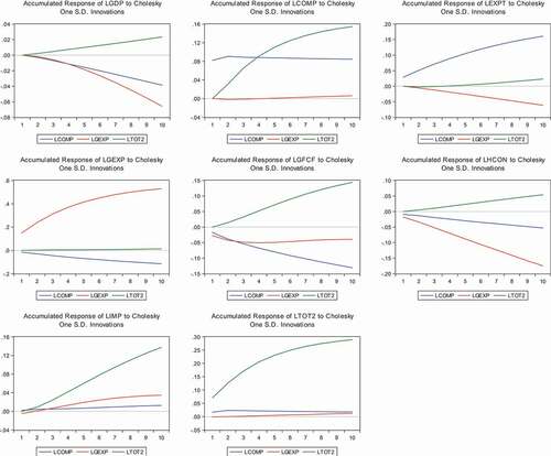
It is evident that a one percent shock to commodity price and Government spending leads to about a negative impact on investment while terms of trade impacts investment positively over the horizon (see Appendix). In the fifth period, a shock to commodity price and Government spending has to a negative impact on investment of −0.80 and −0.49, respectively. As observed in the same period, a percent shock terms of trade brings about a 0.71 percent positive impact on investment. The trend continues over the horizon examined for this study. From examining the response of Government spending to these exogenous shocks, it was observed that commodity price had a negative impact over the horizon. Government spending and terms of trade, however, had a positive impact over the horizon.

In the ninth period, commodity price had a negative impact of −10.7 percent on Government spending. There was a positive impact of 51.6 percent and 10.9 percent from Government spending and terms of trade shocks, respectively, in the same horizon (period). A one percent shock to Government spending has a negative impact of −0.47 in the first period. However, in subsequent periods the impact became positive. Particularly in the third period, Government spending has a positive impact of 0.68 percent on total imports. Commodity price and terms of trade both had a positive impact on total imports. In the seventh period to be precise, commodity price had a positive impact of 0.93 percent, while terms of trade also had a positive impact of 9.45 percent. Terms of trade had a negative impact on total export in the first horizon. However, as the horizons progressed, the impact became a positive one. By the fifth period, a one percent shock in terms of trade had a positive impact of 0.35 percent on total exports. Commodity price exhibited a positive impact on total exports. Government spending, on the other hand, had a negative impact on total exports throughout the horizon. The seventh period, Government spending had a negative impact of −3.99 on total exports. This trend was maintained throughout the horizon considered for the study.

Table 2 presents the results of the variance decomposition of major macroeconomic variables to shocks in commodity price, Government spending and terms of trade. As observed in Table 2, Government spending accounts for the largest variance in real GDP (0.99 percent). In the fifth period, commodity price accounted for 0.63 percent variation in real GDP while terms of trade accounted for 1.05 percent and 0.62 percent in the fourth period, respectively. Terms of trade accounted for the least variance in private consumption.

From observing the variance of shocks to investment, commodity price, Government spending and terms of trade accounted for 1.53 percent, 1.99 percent and 0.40 percent respectively. Government spending also accounts for the largest variance in investment, with 2.39 percent in the first period. Terms of trade, however, accounts for its own largest variation with 84.1 percent in the first period. Then commodity price accounts for about 1.66 percent variation and terms of trade accounts for about 0.014 percent in the fifth period.

The variance decomposition of total imports from Table 2 shows terms of trade accounting for the largest variation (1.81 percent). In comparison, Government spending and commodity price accounted for 0.31 percent and 0.02 percent, respectively in the fifth period. Commodity price appears to account for the largest variance in total exports (2.51 percent). While 0.14 percent and 0.012 percent variations in total exports was accounted for by shocks to government spending and terms of trade as seen in Table 2.

4.1. Discussion

The findings of this study, support the findings of Alege (2008). In effect, commodity prices are observed as the main drivers of terms of trade in developing economies. In Africa exports predominantly depend on a few commodities as compared to other advanced nations. The relevance of terms of trade shocks in Africa is as a result of the high dependence on commodities. Terms of trade may be seen to exhibit a direct relationship with commodity prices. That means when commodity prices increase terms of trade exhibit a corresponding increase, and terms of trade decreases when commodity prices decline. Most African countries are dependent on agricultural commodities and oil for export earnings; therefore, an increase in commodity prices increases export earnings.

Furthermore, with prices of import remaining constant terms of trade improves. An improvement in terms of trade due to increases in commodity prices leads to an increase in other macroeconomic variables such as real output, consumption level, investment spending, exports and imports. Exchange rate, which is seen as the amount of a national currency that is needed in exchange for one unit of another foreign currency, can also be referred to as a major determinant of terms of trade. This, however, may not be the case for African countries as an increase in terms of trade does not necessarily guarantee increased imports and output.

From the definition, the terms of trade shows how much imports a country can purchase given its exports, but that does not necessarily mean the country increases its import spending. The preference factor explains the difference between expectation and behaviour of human beings. Therefore, potential terms of trade may not directly have the same effect as actual terms of trade. The nature of imports and exports from African countries can also explain the reason for the inverse relationship between terms of trade and real output. African countries majorly depend on household consumer goods, machinery and equipment for firms imported from advanced countries. The nature of exports from these African countries, which is mostly agricultural produce cannot adequately compensate for the increase in the price of these foreign commodities. In other words, if the commodity prices of these agricultural products are not increasing at the same or even faster rate than that of these foreign commodities, then the favourable effect of increased commodity prices is lost. Furthermore, an unstable socio-political and economic condition of a country can also result in an adverse effect of favourable terms of trade or increase in commodity prices.

The wealth channel, according to RBC theorists, shows the effects of a favourable government spending shock or fiscal policy shock. Households tend to reduce consumption levels and increase working hours due to the negative wealth effects caused by a positive government spending shock. Real wage also declines as labour supply increases. Inflationary pressures accompany the increase in money supply in the economy. Labourers would instead offer more working hours than leisure hours to make up for the decline in wealth. According to theory, an increase in working hours tends to bring about increased productivity and output. However, as real wages and wealth decline, it has a negative effect on the economy, even in the present state of recession. Therefore, the timing of the individual’s reaction to boost productivity during a recession remains a mystery to economists.

The results obtained from examining the impulse responses of real output to real shocks showed that Commodity price shocks and Government spending shocks has a negative impact on real GDP, while terms of trade shocks has a positive impact. The positive impact of terms of trade is seen across the major macroeconomic variables considered for this study. This implies that there a favourable response from macroeconomic variables to a sudden positive change in terms of trade. Therefore, in Africa, an improvement in terms of trade tends to boost real income, consumption levels and investment through optimism among households and firms due to a positive business expectation. The response of the macroeconomic variables to shocks in terms of trade validates expectation.

The negative response of real GDP to government spending shocks is unexpected. However, the nature of the balance of payment of African countries can explain this inverse relationship. Most African countries borrow huge amounts from international organisations to finance government spending, thereby incurring high-interest rate on repayments (Bello et al., 2020). Therefore, the position on external debt is a possible explanation for the negative impact of government spending shock on real GDP. Government spending was also observed to have a negative impact on export, investment spending and household consumption. The negative impact of commodity price shocks on real output is surprising as an increase in commodity prices, according to theory leads to an increase in real income. A possible explanation for the negative relationship observed between commodity prices, and real GDP can be explained by the high unemployment rates in the region. A high level of unemployment indicates low purchasing power. The weak labour force across African countries shows that an increase in commodity prices may not necessarily increase real output. The import-dependent nature of developing countries may also be a contributing factor to these findings. These economies are mostly classified as low-income countries and are highly dependent on the importation of consumer goods. The import-dependent nature of these economies serves as a limiting factor to positive commodity prices shocks. The variance decomposition results indicate that government spending shocks account for the highest amount of variation in real GDP followed by commodity prices shocks and then terms of trade shocks. This therefore highlights the role of government expenditure across African economies.

5. Conclusion

The Bayesian Panel Vector Autoregressive approach was employed to derive the impact of real shocks (commodity price shocks, government spending shocks, and terms of trade shocks) on business cycles. These exogenous shocks have also been identified as major sources of business cycles in Africa by this study: commodity price shocks, government spending shocks, and terms of trade shocks. A country’s terms of trade refer to the ratio of the country’s export prices to the prices of its imports. The terms of trade measures, the units of imports that can be exchanged for a unit of a country’s exports. Therefore, a favourable increase in the terms of trade of a country indicates an increase in the purchasing power of more imports. This tends to boost real income and increase consumption level in the economy.

Specifically, the study finds that terms of trade shock has the highest positive impact on real business cycles in SSA, while government expenditure has the greatest negative shock on business cycle. Furthermore, in SSA exogenous real shocks are sources of business cycle fluctuations in Africa using the Bayesian panel vector autoregressive approach. It is observed that commodity prices and government spending lead to a negative impact on real output and other macroeconomic variables considered in the study, while terms of trade had a positive impact. The variance decomposition highlights the relative importance of government spending across African countries as it accounts for the largest variations in Real GDP.

In conclusion, the Bayesian PVAR model was used in investigating the impact of real shocks on business cycles. The result findings are in line with theory, as the real shocks incorporated in the study as observed, has a significant influence on the major macroeconomic variables. Therefore, real or productivity shocks drive macroeconomic fluctuations in Africa. Government spending shocks was found to possess the highest impact on Macroeconomic fluctuations across the SSA region. This conforms to a priori expectation, as the Government and its institutions participate immensely in economic activities across SSA countries. Terms of trade shocks and commodity price shocks also impact macroeconomic fluctuations across SSA.

Acknowledgements

The support from Covenant University Centre for Research, Innovation and Discoveries (CUCRID) as well as the Equipment Subsidy Grant from the Alexander von Humboldt Foundation [REF: 3.4-8151/19047] awarded to the Centre for Economic Policy and Development Research (CEPDeR) that facilitated the development of the manuscript are acknowledged. The views expressed are the authors’

Additional information

Funding

The authors received no direct funding for this research.

Notes on contributors

Jeremiah O. Ejemeyovwi

Mr. Barnabas Amu obtained an M.Sc. Economics Degree from Covenant University, Nigeria where he was supervised by Prof. Evans Osabuohien and Prof. Philip Alege. Prof. Evans S. Osabuohien is a Professor of Economics and the Chair, Centre for Economic Policy and Development Research (CEPDeR) at Covenant University, Ota, Nigeria. Prof. Philip Alege is a Professor of Economics and former Dean, College of Management and Social Sciences, Covenant University, Ota, Nigeria. Dr. Jeremiah Ejemeyovwi is a lecturer at Department of Economics and Development Studies, Covenant University and a Research Fellow at CEPDeR. The group’s research activities are guided by an interest to carryout relevant policy and development research to contribute to economic literature and make impact by linking. Research to policy and practice. This study draws from a bigger project on The Real Business Cycle in Africa.

References

- Adeleye, N.,Osabuohien, E.,Bowale, E.,Matthew, O.,& Oduntan, E. (2018). Financial Reforms and Credit Growth in Nigeria: Empirical Insights from ARDL and ECM Techniques. International Review of Applied Economics, 32(6),807-820
- Alege, P. (2008). Macroeconomic Policies and Business Cycles in Nigeria. ( PhD thesis). Department of Economics and Development Studies, Covenant University
- Alege, P. (2009). A business cycle model for Nigeria. CBN Journal of Applied Statistics, 3(1), 85–18. https://www.cbn.gov.ng/out/2012/ccd/cbn%20jas%20volume%203%20number%201_complete.pdf
- Alege, P. O., & Osabuohien, E. S. (2013). G-Localization as a development model: Economic Implications for Africa. International Journal of Applied Economics and Econometrics, 21(1), 41–72. http://eprints.covenantuniversity.edu.ng/id/eprint/3886
- Aleksander, V. (2016). Business Cycles in Bulgaria and the Baltic Countries: An RBC Approach. ( EconStor Theses). ZBW - Leibniz Information Centre for Economics, number 142163.
- Ballabringa, F. C., Gonzalez., L. J. A., & Jareno, J. (2000). A BVAR macroeconomic model for the Spanish economy. Banco de España.
- Bello, H. T., Ayadi, F., Osabuohien, E. S., Ejemeyovwi, J. O., & Okafor, V. (2020). Economic analysis of growth finance and liquid liabilities in Nigeria. Investment Management and Financial Innovations, 17(3), 387–396. https://doi.org/https://doi.org/10.21511/imfi.17(3).2020.29
- Burns, A., & Mitchell, W. (1947). Measuring business cycles. Social Research, 14(3), 370–377. http://www.nber.org/books/burn46-1
- Canova, F. (1994). Statistical inference in calibrated models. Journal of Applied Econometrics, 9(S), 123–144. https://doi.org/https://doi.org/10.1002/jae.3950090508
- Canova, F., & Ciccarelli, M. (2013). Panel vector autoregressive models: A survey. European Central Bank Working Paper Series No 1507, European Central Bank. 1–52.
- Combes, J., Ebeke, C., Etoundi, M. N., & Thierry, Y. U. (2014). Are foreign aid and remittances a Hedge against food price shocks in developing countries? World Development, 54(1), 81–98. https://doi.org/https://doi.org/10.1016/j.worlddev.2013.07.011
- Doan, T., Litterman, R., & Sims, C. (1984). Forecasting and conditional projection using realistic prior distribution. Econometric Review, 3(1), 1–100. https://doi.org/https://doi.org/10.1080/07474938408800053
- Ejemeyovwi, J. O., Osabuohien, E. S. & Bowale, E. I. K. (2020). ICT adoption, innovation and financial development in a digital world: empirical analysis from Africa, Transnational Corporations Review. doi:https://doi.org/10.1080/19186444.2020.1851124
- Gavin, W. T., & Theodorou, A. (2005). A common model approach to macroeconomics: Using panel data to reduce sampling error. Journal of Forecasting, 24(3), 203–219. https://doi.org/https://doi.org/10.1002/for.954
- King, R., & Rebelo, S. (1999). Resucitating real business cycles. In J. B. Taylor & M. Woodford (Eds.), Handbook of macroeconomics (1st ed., pp. 927–1007). Elsevier.
- Kydland, E., & Prescott, E. (1982). Time to build and aggregate fluctuation. Econometrica, 50(6), 1345–1370. https://doi.org/https://doi.org/10.2307/1913386
- Litterman, R. (1986). Forecasting with Bayesian vector auto regressions - Five years of experience. Journal of Business & Economic Statistics, 4(1), 25–38. https://gpe.ufes.br/sites/gpe.ufes.br/files/field/anexo/Forecasting%20with%20Bayesian%20Vector%20Autoregressions%20Five%20Years%20of%20Experience.pdf
- Nason, J. M., & Cogley, T. (1994). Testing the implications of long-run neutrality for monetary business cycle models. Journal of Applied Econometrics, 9(S), 37–70. https://doi.org/https://doi.org/10.1002/jae.3950090504
- National Bureau Statistics (2016). Nigerian gross domestic product report. Retrieved from https://www.nbs.gov.sc/downloads
- Olaniran, O., Oladipo, A., & Yusuff, A. (2017). Business cycle, macroeconomic variables and economic growth in Nigeria (1986-2014); A time series econometric approach. Global Journal of Human-Social Science: Economics, 7(6), 85–95. https://socialscienceresearch.org/index.php/GJHSS/article/view/2420
- Patroba, H., & Raputsoane, L. (2016). South Africa’s real business cycles: The cycle is the trend. Stellenbosch Economic Working Papers: 12/16, Stellenbosch University, Department of Economics, 1–18
- Prescott, E. (1986). Theory ahead of business cycle measurement. Federal Reserve Bank of Minneapolis Quarterly Review, 10(4), 9–22. http://minneapolisfed.org/research/sr/sr102.pdf
- Schorfheide, F. (2000). Loss function-based evaluation of DSGE models. Journal of Applied Econometrics, 15(6), 645–670. https://doi.org/https://doi.org/10.1002/jae.582
- Sims, C., & Zha, T. (1998). Bayesian methods for dynamic multivariate models. International Economic Review, 39(4), 949–968. https://doi.org/https://doi.org/10.2307/2527347
- Sissoko, Y., & Dibooglu, S. (2006). The exchange rate system and macroeconomic fluctuations in Sub-Saharan Africa. Economic Systems, 30(2), 141–156. https://doi.org/https://doi.org/10.1016/j.ecosys.2005.11.002
- World Bank (2020). World development indicators. World Bank Publications https://data.worldbank.org/indicator/NY.GDP.MKTP.KD.ZG?locations=NG (Accessed: 15/ 07/2020).