Estimating the production function for the Brazilian industrial sector: A Bayesian panel VAR approach

Abstract

The scope of this paper is to estimate the production function for the Brazilian industrial sector from a longitudinal panel of the industrial sector (Annual Industrial Survey produced by the Institute of Geography and Statistics—PIA/IBGE—and the Ministry of Labour and Employment’s Annual Relation of Social Information—RAIS/MTE—ranging from 1996 until 2005) through a Bayesian Vector Autoregressive (BVAR) approach. This new method adds to the empirical industrial organization another way to estimate the demand, avoiding cumbersome calculations. It gives the possibility of analysing not only the dynamic relationships among the variables but also the shocks through the impulse response function (IRF). Additionally, it gives the opportunity to analyse the industry sector’s productivity by minimizing the problem of endogeneity and therefore it also sheds some light on the trend of this variable throughout the period abovementioned.

Keywords:

• Bayesian panel vector autoregressive
• production function
• productivity

Subjects:

• L11
• C11
• C32
• C33

PUBLIC INTEREST STATEMENT

The scope of this paper is to estimate the production function for the Brazilian industrial sector from a longitudinal panel of the industrial sector during Real Plan until President’s Lula management through a Bayesian Vector Autoregressive (BVAR) approach. This new method adds to the new empirical industrial organization another way to estimate the demand, avoiding cumbersome calculations such as Olley and Pakes (1996) and Levinsohn and Petrin (2003). It gives the possibility of analysing not only the dynamic relationships among the variables but also innovations through the impulse response function (IRF). Additionally, it gives the opportunity to analyse the industry sector’s productivity by minimizing the problem of endogeneity and therefore it also sheds some light on the trend of this variable. Then, it appoints the idea that human capital itself is not a driver in the Brazilian industry; just for sectors that employ high technological process and requires highly qualified workers.

1. Introduction

The scope of this paper is to estimate the Brazilian production function from a longitudinal panel of the industrial sector (Annual Industrial Survey produced by the Institute of Geography and Statistics—PIA/IBGE—and the Ministry of Labour and Employment’s Annual Relation of Social Information—RAIS/MTE—ranging from 1996 until 2005) through a Bayesian Vector Autoregressive (BVAR) approach. This new method adds to the empirical industrial organization another way to estimate the demand, avoiding cumbersome calculations such as those found at Olley and Pakes (1996) and Levinsohn and Petrin (2003) papers. It also gives the possibility of analysing not only the dynamic relationships among the variables but also the shocks through the impulse response function (IRF). Additionally, it gives the opportunity to analyse the industry sector’s productivity by minimizing the problem of endogeneity and therefore it also sheds some light on the trend of this variable throughout the period abovementioned. One big advantage of using the Bayesian framework relies on the fact that unobservable variables are fully estimated by using the a priori assumption and when this is updated it culminates in a new a posterior distribution.

In item two, it is done a revision of the literature regarding the idea behind Vector Autoregressive theory, mostly used in Macroeconomics. It is rest upon heavily on the Holtz—Eakin’s seminal paper (1988). Afterwards, a brief explanation regarding Bayesian point of view is also outlined, following the suggestion used in LeSage’s Matlab econometrics package and Canova’s book “Methods for Applied Macroeconomic Research”. In the following item, it is explained that the model as well as the retrieval of all variables used within the estimation also pay attention to methodology issues concerning it.

The estimated regression in item four aimed at verifying the dynamic relationship through the Cobb-Douglas production function, accounting for the industrial sector’s input production, that is, salary¹ and capital. As suggested by Olley and Pakes (1996), a certain care was taken in avoiding the selection and endogeneity problem by controlling the number of firms who enter and exit during the timeframe in question. Comparison is made with other estimated methodologies such as Ordinary Least Square (OLS), General Least Square (GLS) and General Method of Moments (GMM). Some interesting findings do not corroborate the analysis of the authors in the aspect of having an overestimating problem with regards to capital and underestimating to labour.

2. Review of the literature

The objective of using the Vector Autoregressive approach (VAR) is related to its parsimony, avoiding cumbersome calculations as, for example, openly used in Olley and Pakes (1996) and Levinsohn and Petrin (2003), which requires a three stage methods to estimate demand functions—and level-based firms’ productivity— of course with variations as proposed by the latter authors, which use an intermediate input (material) as instrumental variables. The basic setup is suggested as follows:

1. Traditional Ordinary Least Square (OLS) regression is made in order to find the coefficient concerning the labour using a fourth order polynomial extension;

2. Analysis of survival through a Probit model;

3. And finally a Nonlinear Least Square (NLS) is performed in order to find the coefficients of capital, given the investment (and material inputs) as instrumental variables and the unobservable factor (which is productivity).

Those structural stages are set up in order to solve the problem of endogeneity towards productivity, which is sorted out between observable and unobservable variables. The first one being the decision-making process made by the board of management; whereas the second one being a truly unpredictable (or unanticipated) shock. However, both are presented as part of the “residuals” within the production function equation. Notwithstanding this rather complicated framework, a couple of assumptions covers both Olley and Pakes (1996) and Levinsohn and Petrin (2003) solutions, which can be subsumed below:

1. Strict monotonicity between the instruments and unobservable productivity;

2. This productivity also enters the instruments equations;

3. Labour does not have a dynamic implication as capital.

A web of science search shows us that firm productivity with panel VAR approach has very few outcomes. In 2018, the results were only 16 articles, while in 2017 accounted only for 11 and 6 in 2016. Overall, the new empirical industrial economics has based their finding in traditional methods, such as linear panel data, maximum likelihood and Arellano-Bond framework. They are shown in Journal of Economic Dynamics and Control (20), Economics Letters (6), Economic Modelling (5). Doing the same search, but only specifying firm productivity estimates using Cobb-Douglas model, articles figures were raised to 409 in 2018, 321 in 2017 and 371 in 2016. Journals that mostly contributed to the above results were essentially Economic Modelling (370), Journal of Economic Dynamics and Control (337) and European Economic Review (308).

It is clear that developing a new approach to the estimation of firm productivity, using panel data allied with non-frequentist time series methods would be a significant contribution to the literature.

In that line of thought, we cite the work of Miranda et al. (2017), which argues that in a traditional Cobb-Douglas model, if only if covariates are correlated with the individual-specific effects and derive appropriate GLS and IV estimators for the resulting correlated random effects spatial panel data model. Also, they provide production function estimates supporting the existence of public capital spillovers, whose relation falls back on the evidence of a relation between public capital and the unobserved productivity (i.e., the individual specific effect of the production function) and its spatial spillover. This fact is not clearly shown in Olley and Pakes (1996), Levinsohn and Petrin (2003), and C. Álvarez et al. (2016) states that production function approach is used to introduce the effect of public infrastructure on economic growth focusing on its spillover effects, being one of them productivity. They also managed to utilize spatial interdependence into these models, applying the most recent spatial econometric techniques based on instrumental variables estimation in spatial autoregressive panel models in comparison with Maximum Likelihood estimation methods. They concluded that in the spatial autoregressive panel model, labor and private capital are relevant production factors. Then, it confirms the relevance and significance of spillovers effects, which is consistent with the new empirical industrial organization.

Mavroeidis et al. (2015) presented a miscellaneous framework, using a maximum likelihood method to estimate the cross sectional distributions of heterogeneous autoregressive (AR) parameters with short panel data. They construct a panel likelihood by integrating unknown cross-sectional density of heterogeneous AR parameters with respect to a known time-series data generating kernel. A model of employment dynamics with the firm-level data of Arellano and Bond (1991) was tested and as a conclusion, they found out that adjustment rates of employment are significantly heterogeneous across firms and this result is not available with the existing methods, since they presume homogeneous adjustment rates or long panel data. In summary, the authors have shown a way to have a more generic and flexible model estimation, avoiding several econometric stages.

3. Methodology

In this article, it will proposed the use of Vector of Autoregressive (VAR), taken the form of as in Holtz-Eakin et al. (1988). The advantage of it is regarding its relative simplicity and flexibility in dealing with econometric problems. Different from the macroeconomic point of view, the micro data have its own idiosyncrasies which accounts for individual’s heterogeneity across the longitudinal panel (cross-section). Pooling cross-section models have the following advantages:

1. Assumption of time stationary can be relaxed, allowing for integrated series if this is the case;

2. Asymptotic theory for large cross-sections units does not require the VAR to have unit or explosive roots (that is, non-stationary), which means the first point of the life of individuals is hypothetically “constant” (or also known as “random walk”).

To a certain point, the abovementioned assumptions are interesting because it provides no restrictions concerning the dynamic relationships among individuals (and those individuals’ movements as time passes by). Most importantly is the fact that allowing for lags from the dependent variable, it solves for the endogeneity problem concerning anticipated or predictable productivity, since it carries over from one time to the subsequent ones, minimizing its impact by giving less relevance to higher lags and therefore the residuals become less correlated to the remaining variables. Henceforth this fact can substitute the three-stage estimation proposed by Olley and Pakes (1996) and Levinsohn and Petrin (2003).

In terms of statistical inferences within the VAR approach, it must hold the orthogonality conditions within the errors and the variables within the system and this will be accomplished by Cholesky decomposition. In addition to it, error correction model can be also estimated in case of a long-term relationship dynamics among the variables.

According to Antonakakisa et al. (2017), the advantages of using a panel VAR methodology relative to other methods are: (i) panel data models allow us to control for unobservable time-invariant characteristics, reducing concerns of omitted variable bias; (ii) time fixed effects can also be added in order to account for any shocks; (iii) the inclusion of variables lags helps to analyse the disequilibrium (or not) relationships among them. In that sense, impulse response functions based on PVARs can account for any delayed effects of the variables under consideration and thus determine whether the effects of those variables are short-lived, long-lived or even both. Such dynamic effects would not have been captured by traditional panel regressions; (iv) PVARs are designed to address the endogeneity problem, which is one of the most serious challenges of any empirical research; and (v) PVARs can be effectively employed with relative short-time series due to the efficiency gained from the cross-sectional dimension.

Moreover, according to Christou et al. (2017), a PVAR model may allow for (i) dynamic interdependencies, which, in turn, occur when one sectoral variable affect another lagged variable, (ii) static interdependencies which occur when the correlations between the VARs’ errors of two or more sector variables are non- zero and (iii) cross-section heterogeneities which happen when two sectors have VARs with different coefficients. Furthermore, given the autoregressive structure of a PVAR, endogeneity problems are solved. Also Koop and Korobilis (2016) developed methods which select among all possible combinations of restricted PVARs and find a parsimonious PVAR which deals with the overparameterization problems.

In Econometrics, it is well-known that one problem related to the micro data is concerning small samples. For that, LeSage’s Matlab Econometrics package and Doam, Litterman and Sims (1984) proposed the use of Bayesian prior information, reflected by the Minnesota prior whose mean and variance are normally distributed and if the former is equal to 1 it reflects its importance in terms of lagged explanatory variables of coefficients of the model and if it is assigned zero is otherwise. This assumption, however, can also be relaxed. With this new framework, it is then presented the Bayesian panel Vector Autoregressive (BVAR).

4. The model

According to Holtz-Eakin et al. (1988), the estimation of the panel Vector Autogressive Moving Average (VARMA (p,q)) will be done using the reduced form, which takes the form of

(1.1) $X_{it}=A_{i1}{X}_{it-1}+A_{i2}{X}_{it-2}+\dots +A_{ip}{X}_{it-p}+B_{i0}{Z}_{it}+B_{i1}{Z}_{it-1}+\dots ++B_{iq}{Z}_{it-q}+u_{it}$(1.1)

where

X_it represents the endogenous variables;

Z_it represents the exogenous variables.

According to Cholesky decomposition (see, Enders (1995) pgs. 302–303), in order to have a complete identification (and therefore guarantee the orthogonality conditions from the residuals that is expectation of the errors are zeros), it must create a linear combination that entails the following:

$\begin{array}{rl}& X_t=A_1{X}_{t-1}+A_2{X}_{t-2}+\dots +A_p{X}_{t-p}+B_0{Z}_t+B_1{Z}_{t-1}+\dots ++B_q{Z}_{t-q}+u_t\\ & \begin{array}{c}{X}_t={\mathrm{\Phi }}_0^{-1}{\mathrm{\Phi }}_1{X}_{t-1}+{\mathrm{\Phi }}_0^{-1}{\mathrm{\Phi }}_2{X}_{t-2}+\dots +{\mathrm{\Phi }}_0^{-1}{\mathrm{\Phi }}_p{X}_{t-p}+{\mathrm{\Phi }}_0^{-1}{\mathrm{\Gamma }}_0{Z}_t+{\mathrm{\Phi }}_0^{-1}{\mathrm{\Gamma }}_1{Z}_{t-1}+\dots ++{\mathrm{\Phi }}_0^{-1}{\mathrm{\Gamma }}_q{Z}_{t-q}+{\epsilon }_t\\ A_t={\mathrm{\Phi }}_0^{-1}{\mathrm{\Phi }}_1;A_2={\mathrm{\Phi }}_0^{-1}{\mathrm{\Phi }}_2;A_p{\mathrm{\Phi }}_0^{-1}{\mathrm{\Phi }}_p;\dots ;B_0={\mathrm{\Phi }}_0^{-1}{\mathrm{\Gamma }}_0;B_1={\mathrm{\Phi }}_0^{-1}{\mathrm{\Gamma }}_1;B_q={\mathrm{\Phi }}_0^{-1}{\mathrm{\Gamma }}_q\end{array}\end{array}$

where ${\epsilon }_t\sim \left(0,\mathrm{\Sigma }\right)$, ${\mathrm{\Phi }}_0^{-1}$ is idempotent and $E\left(u_t{u}_t^{\prime }\right)=E\left({\mathrm{\Phi }}_0^{-1}{\epsilon }_t{\epsilon }_t^{\prime }\mathrm{\Phi }{{ }_0^{-1}}^{\prime }\right)={\mathrm{\Phi }}_0^{-1}E\left({\epsilon }_t{\epsilon }_t^{\prime }\right){\mathrm{\Phi }}_0^{-1^{\prime }}={\mathrm{\Phi }}_0^{-1}{\mathrm{\Lambda }}_t\mathrm{\Phi }{ }_0^{-}{1}^{\prime }=S$

The triangularization can be guaranteed through a linear combination of the type: $S=P_o{P}_0^{\prime }$; where P is an inferior triangular matrix and is also idempotent. Then:

$\begin{array}{rl}& {\mathrm{\Phi }}_0^{-1}{\mathrm{\Lambda }}_t{\mathrm{\Phi }}_0^{-1^{\prime }}=S=P_0{P}_0^{\prime }\\ & {\mathrm{\Phi }}_0^{-1}{\mathrm{\Lambda }}_t{\mathrm{\Phi }}_0^{-1^{\prime }}=P_0{P}_0^{\prime }=P_0\\ & {\mathrm{\Lambda }}_t{\mathrm{\Phi }}_0^{-1^{\prime }}={\mathrm{\Phi }}_0{P}_0\\ & {\mathrm{\Lambda }}_t{\mathrm{\Phi }}_0^{-1^{\prime }}={\mathrm{\Phi }}_0{P}_0\\ & {\mathrm{\Phi }}_0^{-1^{\prime }}={\mathrm{\Phi }}_0\frac{P_0}{{\mathrm{\Lambda }}_t}\\ & {\mathrm{\Phi }}_0^{-1}{\mathrm{\Phi }}_0^{-1^{\prime }}=\frac{P_0}{{\mathrm{\Lambda }}_t}\\ & {\mathrm{\Phi }}_0^{-1}=\frac{P_0}{{\mathrm{\Lambda }}_t}\\ & {\mathrm{\Phi }}_0^{-1}=\frac{P_0}{{\mathrm{\Lambda }}_t}\end{array}$

Then,

${\mathrm{\Phi }}_0^{-1}\left(i,j\right)=\left\{\begin{array}{c}0\Rightarrow i<j\\ 1\Rightarrow i=j\\ P_0\left(i,j\right)/{\mathrm{\Lambda }}_0\left(i,j\right)\Rightarrow i>j\end{array}\right.$

That is for instance, in a generalized form:

(1.2) $\begin{array}{rl}& \left[\begin{array}{c}\begin{array}{cc}1& 0\end{array}\\ \begin{array}{cc}{\mathrm{\Phi }}_0^{21}& 1\end{array}\end{array}\right]\left[\begin{array}{c}{x}_{1t}\\ x_{2t}\end{array}\right]={\mathrm{\Phi }}_1\left[\begin{array}{c}{x}_{1t-1}\\ x_{2t-1}\end{array}\right]+{\mathrm{\Gamma }}_1{Z}_t+\left[\begin{array}{c}{\epsilon }_{1t}\\ {\epsilon }_{2t}\end{array}\right]\\ & {\mathrm{\Phi }}_0{X}_{it}={\mathrm{\Phi }}_1{X}_{it-1}+{\mathrm{\Gamma }}_1{Z}_t+E_{it}\\ & X_{it}={\mathrm{\Phi }}_0^{-1}{\mathrm{\Phi }}_1{X}_{it-1}+{\mathrm{\Phi }}_0^{-1}{\mathrm{\Gamma }}_1{Z}_t+{\mathrm{\Phi }}_0^{-1}{E}_{it}\\ & X_{it}=A_{1t}{X}_{it-1}+B_{1t}{Z}_t+E_{it}\end{array}$(1.2)

The main criticism against VARMA(p,q) models are related to the overparametrization and it reflects only the “reduced form” from a structural model. For the latter critique, a good way to smooth it out is applying the Bayesian VAR (BVAR), where a priori distribution it is calculated for each of the coefficients instead of restrict them to zero, for instance.

Generally speaking, the use of informative priors is to redimensionalise the unrestricted model towards a parsimonious one, therefore reducing the parameter uncertainty within a certain set of random events and improving forecast accuracy. A benchmark application is with regards to the shrinkage prior proposed by Litterman (1979, 1984) and subsequently developed by the University of Minnesota, more specifically Doan, T., Litterman, R., Sims, C. (1984), which is known in the BVAR literature as the “Minnesota prior”. The informativeness of the prior can be set by treating it as an additional parameter, based on a hierarchical interpretation of the model. In summary, the Minnesota prior introduces restrictions in a flexible way since it imposes probability distributions on the coefficients of the VAR which reduce the dimensionality of the problem and, at the same time, give a reasonable account of the uncertainty faced by the Central Bank. The choice of φ is important since if the prior is too loose, overfitting is hard to avoid; while if it is too tight, the data is not allowed to speak.

In order to complete the desired Bayesian framework, the coefficients will vary accordingly to following system:

(1.3) $\begin{array}{rl}& X_{it}=A_{1i}{X}_{it-1}+B_{1i}{Z}_t+E_{it}\\ & B_{1i}={\bar{B}}_{1i}+V_{1i}\end{array}$(1.3)

Where $E_{it}\sim \left(0,{\mathrm{\Sigma }}_E\right),V_{it}\sim \left(0,{\mathrm{\Sigma }}_V\right)$ and priors have a normal probability distribution.

In terms of Impulse Response Function (IRF), the above setup also imposes a similar pass-through shock to the variables, as suggests. Moreover, the question regarding to the lag/leads of the model can be chosen according to the result of ratio likelihood (LR) hypothesis testing as verified by Holtz-Eakin et al. (1988).

According to the Bayesian view, the coefficients allow to be weighted by the Minnesota priors, with the standard deviation having the form:

(1.4) ${\sigma }_{ijk}=\theta w\left(i,j\right)k^{-\varphi }\left(\frac{{\hat{\sigma }}_{uj}}{{\hat{\sigma }}_{ui}}\right)$(1.4)

Where ${\hat{\sigma }}_{ui}$ is the estimated standard error from the univariate autoregression involving i and the scaling factor is the estimated variance of j and i. The remaining variables are the hyperparameters, which reflects the standard deviation of the prior ($\theta$) and the decay of rate, varying from zero to one, as the lag length increases in less importance—$k^{-\varphi }$. Thus, the variance from the above model will be $V_{it}\sim \left(0,{\mathrm{\Sigma }}_{ijk}\right)$ rather than $V_{it}\sim \left(0,{\mathrm{\Sigma }}_V\right)$.

This setup will help consistently recuperate the structural model (production function) and the error will be used to reflect the unobservational productivity of the economy.

4.1. The data

In this study, it is used a sample data from 1996 to 2005 in order to maintain the same monetary policy anchorage, that is, the “Real Plan” and the application of inflation target system with floating exchange rate. It worth noticing that after 2009, a “new development matrix” was applied the Luiz Inacio Lula da Silva’s Government (mandate from 2002 to 2010) and carried out by his successor, Dilma Roussef (mandate from 2010 to 2016), through a credit stimuli and industry subsidies (automobile, textiles and electronics), so as to buffer the subprime contagion into the country.

Therefore, the panel was constructed from Annual Industrial Survey produced by the Institute of Geography and Statistics—PIA/IBGE—and the Ministry of Labour and Employment’s Annual Relation of Social Information—RAIS/MTE—ranging from 1996 until 2005. It was used a 107 disaggregation from sub-sectors of the economic activity according to the CNAE (National Classification of Economic Activity).

Below it can be found the variables retrieved from the above surveys:

1. PRODUCTION (prod)—Earnings from Sales;

2. )LABOUR (lab)—Average Nominal Salary from the year in question;

3. CAPITAL (cap)—Net Fixed Assets in a year (already discounted by the depreciation);

4. INSTRUMENTAL VARIABLE (inst)—Average Nominal Salary from other sectors (except for the one in question);

5. EXIT (exit)—Binary variable that gives 1 to a negative variation of the number of firms;

6. ENTRANCE (ent)—Binary variable that gives 1 to a positive variation of the number of firms.

All non-deterministic variables were deflated by the accumulated annual inflation index calculated by the Brazilian Central Bank (IPCA—IBGE). Firms have the total of employees above 30 people, that is, it has been analysed the small, medium and large enterprises. The avoidance of micro-firms diminishes the strong problem of selection, since its rate of “death” is relatively high, by reaching a foreclosure in the first year, according to SEBRAE survey in 2005.

Turning to the binary variables, exit and entrance might cast some doubts about the possibility of encountering collinearity among the dependence variables. However, this is not seemed to be the case, since there are years, whose variations are zero within the analysed sectors. One can critic this effect because it is not possible to distinguish this zero variation from a transaction between a merger (less 1 one firm) and an entrant (1 additional firm). But this is a problem from Data Generating Process (DGP) because IBGE does not have a plant-based firm database.

It is interesting to show now the dynamics of all sectors pertaining to the panel data in a time average basis, that is, from 1996 to 2005.

The highest level of average production reflects the export sectors from the Brazilian economy, with special attention to Beverages, Food (vegetables and meal), Sugar, Iron Ore, Steel/Metal, and Automobile—represented in great part by the following companies Inbev, JBS, Cosan, Vale, CSN, Petrobras, GM, VM, FIAT and Ford—, as it can be verified in the tables below. Furthermore, they also present a high level of capital stock (in average terms), which suggest that the level of productivity among those sectors through new technologies are relatively low (requiring also certain time for them to mature).

Earnings, however, show a low level of payoff (considering they are not fully labour-intense), except for the automobile industry. This pattern appoints that human capital development is not a driver for the Brazilian industry. Exceptions are those sectors which demands higher labour qualification and they, therefore, offer higher compensations such as the case of Aviation (i.e., Embraer) and Oil derivates (i.e., Petrobras).

From the previous section, the equation which could best describe the dynamics above analysed are the Cobb-Douglas functional form in log terms as of below:

(1.5) $pro{d}_{it}=A_{i1}pro{d}_{it-1}+B_{0t}\mathrm{capita}{l}_{it}+B_{1t}\mathrm{labou}{r}_{it}+B_{2t}ins{t}_{it}+B_{3t}exi{t}_{it}+B_{4}en{t}_{it}+u_{it}$(1.5)

where “i” is the sector analysed, “t” is the time series panel, “A_it” is the lagged dependent variable, “B_0t” to “B_4t” are the exogenous variables and also represent the state space coefficients, according to equation (1.3)(1.3) $\begin{array}{rl}& X_{it}=A_{1i}{X}_{it-1}+B_{1i}{Z}_t+E_{it}\\ & B_{1i}={\bar{B}}_{1i}+V_{1i}\end{array}$(1.3) and assuming (1.4) assumptions.

In the next section, the analysis of the abovementioned estimated equation will take place and some interesting results will be drawn from it.

5. The estimation

The Bayesian panel Vector Autoregressive (BVAR) regression has the recourse of using LeSage’s MATLAB Econometric package and for the comparison with other methodologies (OLS, Fixed Effects, Random Effects, GMM, and GLS).

As it can be seen in Tables 1, 2 and 3 below, although production (prod) and capital (cap) present a high standard deviation (remembering it is in log terms), a test of normality shows that the normal distribution can be rejected at a 5% level of significance. Labour (lab) can also be denoted as normal with the only exception of the instrumental variable, whose has got a probability of rejecting the normality hypothesis around 13%. But this is due to the way this variable was constructed, that is, around an average salary from other sectors and therefore it is less prone to huge dispersion, representing then a leptokurtic form. However, in order to facilitate the analysis, all variables are deemed to be normal, since Chi squared is produced by normal distributions.

Table 1. Average sector output/input results

a
Source: IBGE (National Institute of Statistics and Geography)	Source: IBGE (National Institute of Statistics and Geography)	Source: RAIS/MTE (Ministry of Labour and Employment)
b
Source: IBGE (National Institute of Statistics and Geography)	Source: IBGE (National Institute of Statistics and Geography)	Source: RAIS/MTE (Ministry of Labour and Employment)
c
Source: IBGE (National Institute of Statistics and Geography)	Source: IBGE (National Institute of Statistics and Geography)	Source: RAIS/MTE (Ministry of Labour and Employment)

Table 2. Descriptive statistics

Variable	Mean	Std. Dev.	Min	Max
prod	13.76	3.61	0.00	17.94
lab	6.24	1.17	0.00	8.13
cap	10.89	3.05	0.00	15.81
inst	6.29	0.03	6.24	6.36

Table 3. Normality test (*)

Variable	Pr (Skewness)	Pr (Kurtosis)	chi2 (2)	Prob>chi2
prod	0	0	.	0
lab	0	0	.	0
cap	0	0	.	0
inst	0	0.136	51.6	0

(*) 5% level of significance.

It is worth noticing that all variables are positively correlated, even though on a low value as verified in Table 4Table 5. From this first point of view, it diverges from Olley and Pakes (1996) results in the sense that they verify a negative correlation with regards to capital.

Table 4. Correlation matrix

Variable	prod	lab	cap	inst	prod(-1)lab(-1)		cap(-1)
prod	1
lab	0.371	1
cap	0.952	0.359	1
inst	-0.086	-0.093	-0.0652	1
prod(-1)	0.125	0.017	0.0467	-0.0887	1
lab(-1)	-0.172	-0.031	-0.1681	-0.0786	0.0016	1
cap(-1)	0.054	0.016	0.0662	0.0684	0.7851	0.0073	1

Table 5. Likelihood ratio

No Lags H0	No Lags H1	Statistic	Probability (**)
12	11	1.6177	0.2034
11	10	4.8034	0.0284
10	9	-0.9873	1.0000
9	8	0.0440	0.8338
8	7	47.4348	0.0000
7	6	2.0757	0.1497
6	5	7.1718	0.0074
5	4	9.0597	0.0026
4	3	0.8078	0.3688
3	2	0.0530	1.0000

(*) H0 = ”Full Model” against H1 = ”Restricted Model”

(**) Level of Significance 5%

After the descriptive statistical analysis, now it is necessary to turn to model itself by choosing the lags representing the autoregressive component, according to a Likelihood ratio Hypothesis (LR). It is considered the maximum lag length of 12 and minimum of 3 as it can be shown below. The ideal result achieved is 5 lags.

Now for the Bayesian part, the hyperparameters are set to implement the dissipation of the prior, that is, recalling from section three, tightness is given by theta and equals 1%. The weight is 0.5, which means information from the priors are relatively important. The rate of decay around 1 is a medium “dying out” process. Therefore, running the regressions it yields in the results in Table 3. It is worth noticing that BVAR produces a coefficient in capital whose magnitude is relatively less than the orders estimations. This is an interesting result because the manufacturing industry in Brazil are not fully capital intense in a strict definition, as observed within data in Section 3. It also employs a mix with labour force and capital.

This fact implicates that the high level of average capital stock in the most prominent industries in Brazil does not dominate the data as a whole, since the BVAR regression shows a coefficient of 0.4 (and when comparing to other methodologies, this value is 60% less). That means not only most of the sectors employs low level of capital stock (as seen in Section 3), but it is also carried over to other periods. Considering also the control variables for selection (exit and entrance), coefficients are considerably high too, that is—0.32 and 0.28, respectively. This points to an interesting dynamic:—Firms might improve their level of productivity by “entering” into new markets (or sectors) or alternatively merging or acquiring competitors. Unfortunately, the latter cannot be fully identified owing to the data generating process (DGP) as mentioned before.

However, calculating an estimated productivity a la Olley and Pakes (1996)—where productivity stems from the residuals—, growth (in aggregate terms) is relatively small, with an average increase of 3.9% (CAGR—Compound Annual Growth Rate). It can be verified in Table 6 and Table 7 below.

Table 6. Productivity

Year	% YoY
1997	16.4%
1998	-0.1%
1999	9.3%
2000	0.5%
2001	6.0%
2002	4.4%
2003	1.9%
2004	-0.5%
2005	-1.2%

Table 7. Estimation

SAMPLE	FULL SAMPLE
ESTIMATION	(1) OLS	(2) GMM	(3) GLS	(4) FE	(5) MLE	(6) BVAR
PRODUTO (-1)	-	0.1955	-	-	-	0.7500
st.dev.	-	(0.0317)	-	-	-	(0.0126)
t-stat. (*)		6.1547				59.3839
PRODUTO (-2)	-	-	-	-	-	-0.0490
st.dev.	-		-	-	-	(0.0070)
t-stat. (*)						-6.9773
PRODUTO (-3)	-	-	-	-	-	-0.0176
st.dev.	-		-	-	-	(0.0048)
t-stat. (*)						-3.6414
PRODUTO (-4)	-	-	-	-	-	-0.0084
st.dev.	-		-	-	-	(0.0036)
t-stat. (*)						-2.2986
PRODUTO (-5)	-	-	-	-	-	-0.0053
st.dev.	-		-	-	-	(0.0029)
t-stat. (*)						-1.8068
LABOUR	0.0958	-	0.0455	0.2342	0.1810	0.0626
st.dev.	(0.0291)	-	(0.0710)	(0.0394)	(0.0359)	(0.0413)
t-stat. (*)	3.2868		0.6404	5.9326	5.0383	1.5127
LABOUR (-1)	-	-0.0017	-	-	-	-
st.dev.	-	(0.0782)	-	-	-	-
t-stat. (*)		-0.0217
CAPITAL	1.0936	-	1.0494	1.2341	1.1728	0.4310
st.dev.	(0.0119)	-	(0.0332)	(0.0201)	(0.0175)	(0.0214)
t-stat. (*)	91.1748		31.5364	61.3001	66.7201	20.1290
CAPITAL (-1)	-	1.1356	-	-	-	-
st.dev.	-	(0.0324)	-	-	-	-
t-stat. (*)		35.0099
INST	-2.1044	-1.2880	-2.4448	-1.4123	-1.7997	-2.4753
st.dev.	(0.9892)	(1.1720)	(1.6009)	(0.7844)	(0.7845)	(1.4100)
t-stat. (*)	-2.1273	-1.0989	-1.5271	-1.8003	-2.2941	-1.7555
EXIT	0.4222	-0.1322	0.1466	0.0978	0.1725	0.3178
st.dev.	(0.0930)	(0.1433)	(0.1556)	(0.0779)	(0.0778)	(0.1326)
t-stat. (*)	4.5355	-0.9223	0.9415	1.2549	2.2167	2.3951
ENTRANCE	0.4586	-0.0965	0.1177	0.1175	0.1902	0.2860
st.dev.	(0.0964)	(0.1442)	(0.1467)	(0.0803)	(0.0803)	(0.1375)
t-stat. (*)	4.7557	-0.6693	0.8024	1.4626	2.3676	2.0801
CONSTANT	14.1276	0.0033	17.1379	7.6487	11.0249	14.7724
st.dev.	-6.2390	(0.0164)	(10.1848)	(4.9903)	(4.9786)	(8.8887)
t-stat. (*)	2.2644	0.1999	1.6827	1.5327	2.2144	1.6619
R_SQUARED	0.9189	-	0.5240	0.9166	-	0.8368
OBS	1070	1070	1070	1070	1070	1070
* 5%of significance

In the case of labour, it can be verified it reflects negative bias as shown in other regressions (BVAR, OLS and GLS when compared to FE and MLE). This stems from the fact that DGP (Data Generating Process) has some flaws in the sense that in does not open all the employment feature of the firms in the panel. But it corroborates the idea that human capital itself is not a driver in the Brazilian industry (just for sectors that employ high technological process and requires highly qualified workers as shown previously in the dataset (Figure 1)).

Figure 1. Impulse response.

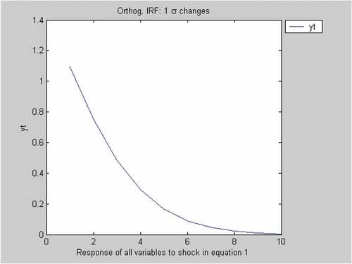
Given that BVAR better describes the dynamics and idiosyncrasies of the Brazilian industrial sector, it is now interesting to analyse “shocks” to productivity in the equation. This is done by considering the impulse response function (IRF). Below in the chart, it is shown that productivity innovations of 1% of standard deviation (that is, 0.55) do not have a permanent impact in production, since it dies out after 10 years in an almost equally paced velocity. This dynamic has a significant meaning because gains in productivity are normally seen in the first periods and the remaining will be absorbed in learning—by—doing process.

6. Concluding remarks

In this paper, it has been presented some interesting results to shed some lights on the estimating the production function from a different and relatively new instrument, that is, the Bayesian Panel Approach. A further line of research will be considering the productivity as an unobservable variable vis-à-vis Kalman Filter (KF). Also, a panel BVAR can be represented by MCMC in case variables a non-linear and non-Gaussian.

Therefore, the scope of this paper is to incentive a further analysis within the new empirical Organisation theory and by avoiding cumbersome calculations such as Olley and Pakes (1996) and Levinsohn and Petrin (2003). It also gives the possibility of analysing not only the dynamic relationships among the variables but also the shocks through the impulse response function (IRF) as seen previously.

Disclosure statement

No potential conflict of interest was reported by the author(s).

Additional information

Funding

The author received no direct funding for this research.

Notes on contributors

Roberto Ivo Da Rocha Lima Filho

My name is Roberto and I am currently an Adjunct Professor at Federal University of Rio de Janeiro in Brazil, teaching economics and principles of finance for engineering undergraduate as well as postgraduate (executive MBAs) students with a myriad of background in the job market.

I deposited my doctorate thesis for a PhD in Science at the University of São Paulo, Medical School, in early 2014. Under the Department of Pathology/Medical Informatics, I managed to better understand the decision making process from traders and students with no financial background with a Neuroeconomics perspective, which is a novelty in the field of finance and economics.

I graduated in Economics in 2000 at the same University and while I was working within the financial markets, I got accepted to the University of Oxford, Queen Elizabeth House, to do a Msc in Economics for Development. After my background within the Financial Markets, I decided to pursue my career in the academia.

Notes

1. In this article, salaries, compensations and earnings are used commonly as synonyms.

Appendix

The algorithms are presented below for both MATLAB and STATA:

M-File MATLAB

% Panel VAR Calculation

nlags = 5; tight = 0.01; weight = 0.5; decay = 1.0; yt = data (:,3); xt = data (:,4:8);

result = bvar(yt,nlags,tight,weight,decay,xt);

prt(result);

% Impulse Response Function

nperiod = 10;

[m1 m2] = irf(result,nperiod,’o1’,’yt’);

Do-File STATA

label data “pia”

tsset sec year

sktest prod lab cap inst

regress prod lab cap inst ent exit

xtreg prod lab cap inst ent exit, fe

xtreg prod lab cap inst ent exit, mle

xtabond prod lab cap, diffvars(lab cap) inst(inst) lags(1) artests(2)

xtgls prod lab cap inst ent exit, panels(correlated) corr(ar1)

sqreg prod lab cap inst ent exit, quantiles(50) reps(20)

References

- Antonakakisa, N., Cunado, J., Filis, G., & Gracia, F. P. (2017). Oil dependence, quality of political institutions and economic growth: A panel VAR approach. Resources Policy, 53, 147–16. doi:10.1016/j.resourpol.2017.06.005
- C. Álvarez, I., Barbero, J., & L. Zofío, J. (2016). A spatial autoregressive panel model to analyze road network spillovers on production. Transportation Research Part A, 93, 83–92. doi:10.1016/j.tra.2016.08.018
- Christou, C., Cunado, J., Gupta, R., & Hassapis, C. (2017). Economic policy uncertainty and stock market returns in Pacific-Rim countries: Evidence based on a Bayesian Panel VAR Model. Journal of Multinational Financial Management, 40, 92–102. https://doi.org/10.1016/j.mulfin.2017.03.001
- Doan, T., Litterman, R.B., and Sims, C.A. (1984). Forecasting and Conditional Projection Using Realistic Prior Distribution. Econometric Review, 3, 1–100. https://doi.org/10.1080/07474938408800053
- Enders, W. (1995). Applied econometric time series. Wyley.
- Holtz-Eakin, D. N., W. Rosen, H., & Rosen, H. S. (1988). Estimating vector autoregressive with panel data. Econometrica, 56(6), 1371–1395. https://doi.org/10.2307/1913103
- Koop, G., & Korobilis, D. (2016). Model uncertainty in panel vector autoregressive models. European Economic Review, 81, 115–131. https://doi.org/10.1016/j.euroecorev.2015.09.006
- LeSage, J. (1999). Applied econometrics using MATLAB. MATLAB Toolbox. https://www.spatial-econometrics.com/html/mbook.pdf
- Levinsohn, J., & Petrin, A. (2003). Estimating production functions using inputs to control for unobservables. Review of Economic Studies, 70(2), 317–342. https://doi.org/10.1111/1467-937X.00246
- Litterman, R. (1979). Techniques of forecasting using vector autoregressions. Federal Reserve Bank of Minneapolis Working Paper. no. 115: pdf.
- Litterman, R. (1984). Specifying VAR’s for macroeconomic forecasting. Federal Reserve Bank of Minneapolis Staff report. no. 92.
- Manuel Arellano, and Stephen Bond. (1991). Some Tests of Specification for Panel Data: Monte Carlo Evidence and an Application to Employment Equations. The Review of Economic Studies, 58(2), 277–297. http://www.jstor.org/stable/2297968
- Mavroeidis, S., Sasaki, Y., & Welch, I. (2015). Estimation of heterogeneous autoregressive parameters with short panel data. Journal of Econometrics, 188(1), 219–235. https://doi.org/10.1016/j.jeconom.2015.05.001
- Miranda, K., Martínez-Ibañez, O., & Manjón-Antolín, M. (2017). Estimating individual effects and their spatial spillovers in linear panel data models: Public capital spillovers after all? Spatial Statistics, 22, 1–17. https://doi.org/10.1016/j.spasta.2017.07.012
- Olley, G., & Pakes, A. (1996). The dynamics of productivity in the telecommunications equipment industry. Econometrica, 64(6), 1263–1297. https://doi.org/10.2307/2171831