The US dollar and trade balance: New findings from the international trade of India with the European Union

Abstract

The US dollar is the most prevalent currency to settle internationally traded merchandise. A few existing studies demonstrate that the US dollar can significantly impact a country’s trade balance with a non-US partner. Nevertheless, the current literature indicates the remarkable deficiency of empirical results for the case of India despite the vital importance of the US dollar in its international trade. Recognizing the European Union (EU) as the largest trading partner of India over the 2000Q1–2022Q2 period, this study is the first to explore how the US dollar influences India’s trade balance with the EU by employing the Nonlinear Autoregressive Distributed Lag (NARDL) method. The results show that, no matter if the US dollar is employed, the depreciation of rupee cannot facilitate India’s trade balance, and the appreciation has a negative effect. Therefore, devaluation is an ineffectual policy for supporting India’s trade balance with the EU.

Keywords:

• EU
• India
• nonlinear
• rupee
• trade balance
• US dollar

JEL classification:

• F10
• F31
• F40

1. Introduction

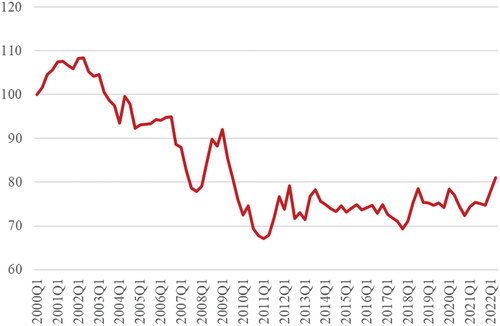
Regardless of the participation of the US, the US dollar is frequently used for settling the goods traded between almost any two countries in the world (Boz et al., 2022). The US dollar is so dominant in the global trade that even large economies substantially depend on its role as an invoicing currency. For instance, while roughly 86% of Indian’s total trade value is invoiced by the US dollar (Gopinath, 2017; Rajan & Yanamandra, 2015), and that number is very noteworthy as the US occupies only around 9.6% of India’s total trade value.¹ Most of the Indian’s trade value with non-US partners, therefore, is settled by the US dollar. Accordingly, the exchange rate between the US dollar and the rupee can affect India’s trade balance with the US as well as the non-US partners. Figure 1 depicts the real exchange rate index between the US dollar and the rupee in the period 2000Q1-2022Q2. There was a sharp downward trend of the index from 2000 to 2011, indicating the appreciation of the rupee against the US dollar. After the first quarter of 2012, the value of rupee in comparison with the dollar was rather stable.

Figure 1. The real exchange rate index between the US dollar and the Indian rupee from 2000Q1 to 2022Q2.

Source: The authors’ computation from the International Financial Statistics (IFS) of IMF.

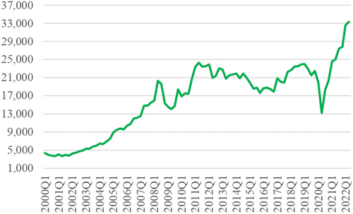
The impacts of the exchange rate between the dollar and the rupee on India’s trade balance with the US have been analyzed by several papers (e.g., Arora et al., 2003; Dash, 2013). Nevertheless, whether it has any influence on the trade balance of India with a non-US country remains a void in the current literature. This research gap motivates this paper to scrutinize the possible effects of the dollar-rupee exchange rate on India’s trade balance with a non-US partner. And we select the EU because it has been the largest trading partner of India for more than two decades. Namely, India’s total trade value with the whole EU was respectively 1.25 and 1.27 times as much as those with China and the US over the period 2000Q1–2022Q2.² Furthermore, the EU altogether consumed India’s products more than any other country across the globe in the same period. Additionally, in June 2022, given the importance of EU-India trade as well as the current restrictive trade regulations in India, the EU resumed the negotiation with India about the free trade agreement (European Commission, 2022). Besides, the investment protection and geographical indications agreements can also enhance the EU-India trade and contribute to the sustainable development (European Commission, 2022). Figures 2 and 3 describe India’s trade balance (measured by exports/imports) and trade value (i.e., exports + imports) with the EU from the first quarter of 2000 to the second quarter of 2022. It can be observed that from 2000Q1 to 2018Q1, India’s trade balance with the EU was mainly in the deficit region (i.e., where the exports/imports ratio is smaller than 1). However, during 2018Q3–2022Q2, there was a strong upward trend in the trade balance, and especially from 2019Q1, it was always in the surplus region. The first quarter of 2022 witnessed the record trade surplus of India with the EU when its exports was 1.55 times more than its imports. During the COVID-19 pandemic, India’s trade value drastically fell by nearly 38.4%. Nevertheless, the trade value quickly recovered and surpassed 33,000 million US dollars in the second quarter of 2022.

Figure 2. India’s trade balance (exports/imports) with the EU from 2000Q1 to 2022Q2.

Source: The authors’ computation from the Direction of Trade Statistics (DOTS) of IMF.

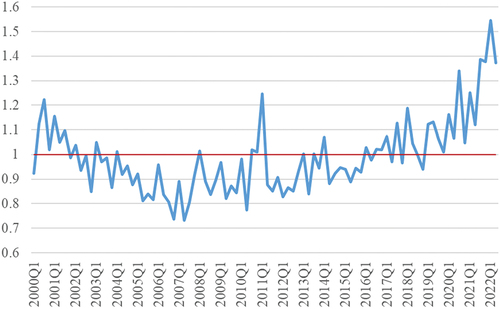
Figure 3. India’s total trade value with the EU during 2000Q1–2022Q2 (million US dollars).

Source: The authors’ computation from the IFS of IMF.

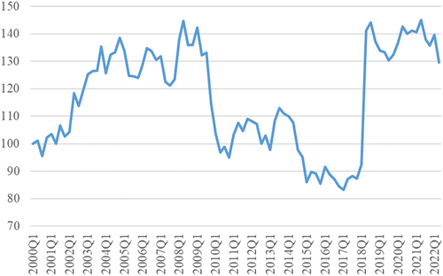
The main objective of this paper is exploring the new evidence for the role of the US dollar in India’s trade balance with the EU over the period 2000Q1-2022Q2. Specifically, the role of the US dollar (reflected by the dollar-rupee exchange rate) is analyzed. Further, to enable more detailed analyses, the effects of the dollar-rupee exchange rate (denoting the usage of the US dollar in the India-EU trade) are compared with those of the EU’s currencies-rupee exchange rate which denotes the non-utilization of the US dollar in the India-EU trade (see Figure 4). Thus, we can observe the different responses of India’s trade balance with the EU under the influences of different invoicing currencies. Besides, due to the application of the NARDL method, the short-run and long-run asymmetric effects of rupee depreciation and rupee appreciation against the US dollar or the EU’s currencies can be clearly revealed.

Figure 4. The real exchange rate index between the EU’s currencies and the rupee from 2000Q1 to 2022Q2.

Source: The authors’ computation from the IFS dataset of IMF.

New contributions to the existing field of research are provided by this article. To begin with, this article realizes the shortage of the empirical evidence for the role of the US dollar in the trade of India with a non-US partner, which is a gap not covered by any existing study. Therefore, this article is the first to explore how the US dollar affects India’s trade balance with a non-US partner. Moreover, this article is also the first to present the empirical evidence for the influences of the US dollar on India’s trade balance with the EU—the largest trading partner of India over the period 2000Q1-2022Q2. Besides, instead of solely analyzing how the dollar-rupee exchange rate impacts India’s trade balance with the EU, this article also scrutinizes the effects of the EU’s currencies-rupee exchange rate. Accordingly, the role of the US dollar is investigated in more details as the trade balance of India with the EU can response differently when it is used for invoicing the goods (reflected by the dollar-rupee exchange rate) and when it is not used (reflected by the EU’s currencies-rupee exchange rate). Additionally, this article employs the NARDL method that can estimate the asymmetric reactions of India’s trade balance with the EU under the depreciation and appreciation of the rupee, which is helpful for identifying novel findings and practical implications regarding the devaluation policy and the selection of invoicing currencies, especially the role of the US dollar, in India-EU trade.

The structure of this article is organized in five sections: Introduction, Literature Review, Materials and Methods, Empirical Results, and Conclusions. The second section summarizes the theoretical frameworks and notable empirical studies in the field of research. The third section (Materials and Methods) demonstrates the sources and the description of variables, the empirical models, and the estimation process of the NARDL method. The fourth section reports the empirical findings about the role of the US dollar in India-EU trade. The final section displays the concluding remarks, the limitation of this article, and the suggestion for future research.

2. Literature review

2.1. The review of major theoretical frameworks

The Marshall-Lerner condition (Lerner, 1944; Marshall, 1923), the J-curve effect (Magee, 1973), and the two-country model (Rose & Yellen, 1989) are normally considered the main theoretical frameworks for researching the impacts of an exchange rate on a trade balance. All the aforementioned frameworks assume that a country uses its currency to invoice its exports to a trading partner. Thus, in the trade between two countries, their currencies are utilized, and a third-country’s currency is absent. Additionally, the depreciation of a country’s currency is expected to facilitate its trade balance. According to the Marshall-Lerner condition, a country’s trade balance is fostered by the depreciation of its currency when the import elasticity of demand in absolute value plus the export counterpart is greater than one. However, the Marshall-Lerner condition is only applicable in the long run, and therefore, the response of the trade balance in the short run cannot be explained. Magee (1973) demonstrated that the trade balance could deteriorate in the short run and then grow in the long run, and he proposed the J-curve effect to explain this phenomenon. Specifically, Magee (1973) expounded the J-curve effect as follows: during the currency-contract and pass-through periods following the devaluation, the import and export quantities cannot promptly change, and consequently the trade balance may decline until the quantities are flexibly adjusted in the long run; and if the Marshall-Lerner condition is satisfied, the trade balance will rise and become surplus. The J-curve effect does not always happen because there are two prerequisites: the reduction of the trade balance in the short run and the occurrence of the Marshall-Lerner condition in the long run. Thus, in order to study the J-curve effect, both the short-run and long-run impacts of the exchange rate on the trade balance must be examined. The current literature demonstrates that the two-country model (Rose & Yellen, 1989) is the popular theoretical framework for conveniently researching the J-curve effect as well as the Marshall-Lerner condition. Rose and Yellen (1989) indicated that a cointegration technique can be applied to estimate the short-run and long-run effects. If the short-run and long-run effects are negative and positive, respectively, the J-curve phenomenon is identified. Moreover, in case the long-run effect is positive, the Marshall-Lerner condition is supported (Bahmani-Oskooee & Kanitpong, 2017; Rose, 1991). Due to the convenience of the two-country model developed by Rose and Yellen (1989), most studies have utilized it for inspecting the exchange rate-trade balance relationship (Baek & Koo, 2009; Bahmani-Oskooee & Aftab, 2018).

The drawback of the aforesaid frameworks is the neglection of a third-country’s currency. This limitation is very crucial in the global trade dominated by the US dollar. Specifically, it is very usual that the US dollar is utilized to settle the trade between any two non-US countries (Boz et al., 2022; Goldberg & Tille, 2008). The heavy dependence on the US dollar can strongly impact the trade of a country with its non-US partners (Gopinath et al., 2020). As a result, the role of the US dollar is so prominent that it cannot be overlooked. Nevertheless, the role of the US dollar in influencing a country’s trade balance with a non-US country is still ignored by the conventional theoretical frameworks (e.g., the Marshall-Lerner condition, the J-curve effect, and the two-country model). Recently, Bao and Le (2022a, 2022b) suggested that the two-country model developed by Rose and Yellen (1989) can be expanded to allow the examination of the US dollar’s role in the trade between two non-US partners.

2.2. The review of relevant empirical studies

India is a large economy in the world with a huge population. Thus, it is not surprising when the relationship between exchange rates and the trade balances of India has drawn much attention from scholars. And most of the existing studies have focused on India’s trade balances with the major individual trading partners of India such as the US, the UK, Germany, China, etc. For instance, Arora et al. (2003) employed the ARDL method to analyzed the impacts of exchange rates on India’s trade balances with the US alongside the UK, Japan, Italy, Germany, France, and Australia over the period 1977Q1-1998Q4. They found that the depreciation of rupee against the US dollar had an insignificant effect on India’s trade balance with the US. And similar results were found in India’s trade with France and the UK. However, the depreciation of rupee against Australian dollar, Japanese yen, Italian lira, and Deutsche Mark fostered India’s trade balances with Australia, Japan, Italy, and Germany. Bahmani-Oskooee and Saha (2017) utilized the NARDL method to scrutinize India’s trade balances with 14 major partners. The results indicated that India’s trade balance with China in the period 1999Q1-2014Q4 was not responsive to the depreciation or the appreciation of the rupee against Chinese yuan. Meanwhile, India’s trade balance with the US between 1973Q1 and 2014Q4 was boosted by the depreciation of the rupee against the US dollar, and the remaining 12 trading partners had mixed outcomes. Chaudhuri (2005) and Islam et al. (2016) also witnessed the positive impacts of the depreciation of the rupee against the US dollar on India’s trade balance with the US. Dash (2013) employed the VECM model and the 1991M1–2005M6 data to examine the bilateral trade of India with the US, Germany, Japan, and the UK. Their findings indicated the J-curve effect in India’s trade with the US, Germany, Indonesia, Japan, Korea, Switzerland, and the UK, which signifies that the depreciation of rupee against the partners’ currencies fostered India’s trade balances.

Many other studies focused on validating the effectiveness of rupee depreciation on India’s total trade balance with the world. For example, Bahmani-Oskooee (1985) found no significant influence of the rupee depreciation on India’s total trade balance, which is in line with the results of Bahmani-Oskooee and Malixi (1992), Bahmani-Oskoee and Alse (1994), and Buluswar et al. (1996). However, Himarios (1989) documented that the depreciation of rupee stimulated India’s trade balance with the world in the periods 1953–1973 and 1975–1984. Lal and Lowinger (2002) utilized the Johansen-Juselius cointegration method for inspecting India’s trade balance with the world over the period 1985Q1-1998Q4, along with some countries including Bangladesh, Nepal, Pakistan, and Sri Lanka. They reported that the depreciation of the Indian rupee and Pakistan rupee encouraged the trade balances of India and Pakistan. In addition, the J-curve effect was observed in Pakistan. Singh (2002) also applied the Johansen -Juselius cointegration method and found that the depreciation of rupee stimulated India’s trade balance during 1960–1995. However, the results were sensitive to the calculation of the exchange rates. Hassan et al. (2017) used the ARDL approach and documented that the depreciation of rupee had no influence on India’s trade balance in the long run over the period 1972–2013. Bhat and Bhat (2021) applied the NARDL method to inspect the exchange rate-trade balance nexus of India. By scrutinizing the monthly data between 1996 M2 and 2017M4, they found that the depreciation of rupee stimulated India’s trade balance.

Rajan and Yanamandra (2015) recognized the prominence of the US dollar as India’s most utilized invoicing currency, but they examined India’s trade balance with the rest of the world which included the US. Some recent studies such as Bao et al. (2022) investigated the importance of the US dollar in the trade of China with a non-US partner. Specifically, Bao et al. (2022) found that China’s trade balance with the EU was significantly affected by the dollar-yuan exchange rate. To the authors’ knowledge, no research has inspected the role of the US dollar in the trade of India with a non-US partner.

3. Materials and methods

This paper uses the quarterly data between 2000Q1 and 2022Q2 collected from reliable sources. Table 1 contains the description and explanation of the variables and their sources. Namely, the exports and imports values of India with respect to the EU, which are used for calculating the trade balance, are downloaded from the Direction of Trade Statistics (DOTS) provided by the International Monetary Fund (IMF) (https://data.imf.org/?sk=9D6028D4-F14A-464C-A2F2-59B2CD424B85). The data about exchange rates and consumer price indices, which are used for calculating the variables REX and RUX mentioned in the Equations 1(1) $\begin{array}{c}ln\mathit{\text{BO}}{T}_t=\alpha +\beta .ln\mathit{\text{RU}}{X}_t+\gamma .ln\mathit{\text{IR}}{I}_t+\delta .ln\mathit{\text{ER}}{I}_t+{\epsilon }_t\end{array}$(1) and 2(2) $\begin{array}{c}\mathit{\text{lnBO}}{T}_t=\alpha {\hspace{0.17em}}^{\mathrm{\prime }}+\beta {\hspace{0.17em}}^{\mathrm{\prime }}.\mathit{\text{lnRE}}{X}_t+\gamma {\hspace{0.17em}}^{\mathrm{\prime }}.\mathit{\text{lnIR}}{I}_t+\gamma {\hspace{0.17em}}^{\mathrm{\prime }}.\mathit{\text{lnER}}{I}_t+{\epsilon {\hspace{0.17em}}^{\mathrm{\prime }}}_t\end{array}$(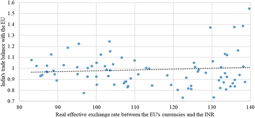2) , are collected from the International Financial Statistics (IFS) dataset provided by IMF (https://data.imf.org/?sk=4c514d48-b6ba-49ed-8ab9-52b0c1a0179b). The real gross domestic products of India and the EU countries are retrieved from the Federal Reserve Economic Data (FRED) of the Federal Reserve Bank of St. Louis (https://fred.stlouisfed.org). The scatter plots indicating the linkage between the exchange rates and the trade balance of India with the EU are given in Figures 5 and 6 in the Appendix section.

Table 1. The description of data

Variable	Description	Measurement	Source
BOT	India’s trade balance with the EU	The ratio Exports/Imports	DOTS
IRI	India’s real income	India’s real GDP	FRED
ERI	The EU’s real income	The weighted average of EU member countries’ real GDPs adjusted by their respective trade shares with India	FRED, IFS, DOTS
REX	The real exchange rate between the EU’s currencies and the rupee	The weighted average of the real bilateral exchange rates between each EU country’s currency and the rupee adjusted by their respective trade shares with India. An increase in REX indicates the depreciation of the rupee.	IFS, DOTS
RUX	The dollar-rupee real exchange rate	The real exchange rate between the US dollar and the rupee. An increase in RUX indicates the depreciation of the rupee.	IFS

Figure 5. The scatter plot between the dollar-rupee real exchange rate index and India’s trade balance with the EU during 2000Q1–2022Q2.

Source: The authors’ computation from the DOTS and IFS of IMF.

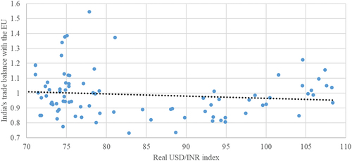
Figure 6. The scatter plot between the EU’s currencies-rupee real exchange rate index and India’s trade balance with the EU during 2000Q1–2022Q2.

Source: The authors’ computation from the DOTS and IFS of IMF.

Following Rose and Yellen (1989), Singh (2002), Arora et al. (2003), Bahmani-Oskooee and Saha (2017), and Bao et al. (2022), this paper uses the following empirical model to investigate the role of the US dollar in India’s trade balance with the EU:

(1) $\begin{array}{c}ln\mathit{\text{BO}}{T}_t=\alpha +\beta .ln\mathit{\text{RU}}{X}_t+\gamma .ln\mathit{\text{IR}}{I}_t+\delta .ln\mathit{\text{ER}}{I}_t+{\epsilon }_t\end{array}$(1)

In Equation 1(1) $\begin{array}{c}ln\mathit{\text{BO}}{T}_t=\alpha +\beta .ln\mathit{\text{RU}}{X}_t+\gamma .ln\mathit{\text{IR}}{I}_t+\delta .ln\mathit{\text{ER}}{I}_t+{\epsilon }_t\end{array}$(1) , BOT represents India’s trade balance with the EU, which is measured by the proportion of India’s exports to imports. The variable RUX denotes the real exchange rate between the US dollar and the rupee. When the coefficient$\beta$ is positive, the depreciation of rupee against the US dollar facilitates India’s trade balance. Next, the variable IRI denotes the real income of India, computed by adjusting its gross domestic product (GDP) by the consumer price index. The sign of $\gamma$ is presumed to be negative, indicating that an increase in India’s income leads to more imports and worsens its trade balance. Similarly, the variable ERI symbolizes the real income of the EU, measured by taking the trade-share-weighted average of their real GDPs. The coefficient $\delta$ is supposed to be positive, signifying that the income of the EU boosts India’s exports and stimulates its trade balance. Besides, all the variables are transformed into indices in which the base period (2000Q1) is set to 100. Then, they are converted into natural logarithm so that the regression coefficients can be interpreted as percentage changes.

The following empirical model indicates the impact of the non-usage of the US dollar on India’s trade balance with the EU:

(2) $\begin{array}{c}\mathit{\text{lnBO}}{T}_t=\alpha {\hspace{0.17em}}^{\mathrm{\prime }}+\beta {\hspace{0.17em}}^{\mathrm{\prime }}.\mathit{\text{lnRE}}{X}_t+\gamma {\hspace{0.17em}}^{\mathrm{\prime }}.\mathit{\text{lnIR}}{I}_t+\gamma {\hspace{0.17em}}^{\mathrm{\prime }}.\mathit{\text{lnER}}{I}_t+{\epsilon {\hspace{0.17em}}^{\mathrm{\prime }}}_t\end{array}$(2)

In Equation 2(2) $\begin{array}{c}\mathit{\text{lnBO}}{T}_t=\alpha {\hspace{0.17em}}^{\mathrm{\prime }}+\beta {\hspace{0.17em}}^{\mathrm{\prime }}.\mathit{\text{lnRE}}{X}_t+\gamma {\hspace{0.17em}}^{\mathrm{\prime }}.\mathit{\text{lnIR}}{I}_t+\gamma {\hspace{0.17em}}^{\mathrm{\prime }}.\mathit{\text{lnER}}{I}_t+{\epsilon {\hspace{0.17em}}^{\mathrm{\prime }}}_t\end{array}$(2) , the variable REX stands for the real exchange rate between the EU’s currencies and the rupee, which is calculated from the real bilateral exchange rates between each currency of the EU countries and the rupee adjusted by their respective trade shares. The rise of REX indicates the depreciation of the rupee. Thus, if $\beta {\hspace{0.17em}}^{\mathrm{\prime }}$ is positive, the depreciation of the rupee improves India’s trade balance. The meanings of the other variables and their respective coefficients in Equation 2(2) $\begin{array}{c}\mathit{\text{lnBO}}{T}_t=\alpha {\hspace{0.17em}}^{\mathrm{\prime }}+\beta {\hspace{0.17em}}^{\mathrm{\prime }}.\mathit{\text{lnRE}}{X}_t+\gamma {\hspace{0.17em}}^{\mathrm{\prime }}.\mathit{\text{lnIR}}{I}_t+\gamma {\hspace{0.17em}}^{\mathrm{\prime }}.\mathit{\text{lnER}}{I}_t+{\epsilon {\hspace{0.17em}}^{\mathrm{\prime }}}_t\end{array}$(2) are analogous to their counterparts in Equation 1.(1) $\begin{array}{c}ln\mathit{\text{BO}}{T}_t=\alpha +\beta .ln\mathit{\text{RU}}{X}_t+\gamma .ln\mathit{\text{IR}}{I}_t+\delta .ln\mathit{\text{ER}}{I}_t+{\epsilon }_t\end{array}$(1)

The choice of an estimation method is very important in an empirical study. Different estimation methods have dissimilar requirements on the characteristics of data. For instance, the well-known Engle-Granger and Johansen-Juselius cointegration techniques are only workable when the variables are I(1) series. Thus, if there are both I(1) and I(0) series, the aforesaid techniques cannot be used, and we must use a more flexible method such as the NARDL method. The motivations for the usage of the NARDL method (Shin et al., 2014) in this paper are threefold. First, it is endowed with all the advantages of the conventional ARDL method such as the allowance for both I(1) and I(0) variables and the suitability for small sample size (Pesaran et al., 2001; Rahman & Ahmad, 2019). Second, the NARDL is the extension of the ARDL method, and thus it provides more flexibility when an increase and a decrease of an independent variable can have different effects on the dependent variable in terms of sign and size. On the contrary, the ARDL method restricts that if a 1% increase in X boosts Y by 0.5%, then a 1% decrease in X must reduce Y by 0.5%. Due to this limitation of the ARDL method, the NARDL counterpart is more superior and can better reflect economic relationships because asymmetry is a notable feature of economic data (Chen et al., 2020; Liang et al., 2019). And the superiority of the NARDL method is well recognized in the literature regarding the impacts of exchange rates on trade balances. As criticized by the pioneering and influential work of Bahmani-Oskooee and Fariditavana (2015, 2016), the symmetric assumption about the exchange rate-trade balance relationship is a common limitation of the prior studies, which contributes to the inadequacy of significant results. And this is the reason why virtually all subsequent published articles employed the NARDL method and affirmed its usefulness (e.g., Bahmani-Oskooee & Nasir, 2020; Iyke & Ho, 2018; Nusair, 2017). Third, recent studies about the role of the US dollar in determining the trade balances of some emerging markets also demonstrated the asymmetric impacts in both the short run and long run (e.g., Bao & Le, 2021a).

The Equations 1(1) $\begin{array}{c}ln\mathit{\text{BO}}{T}_t=\alpha +\beta .ln\mathit{\text{RU}}{X}_t+\gamma .ln\mathit{\text{IR}}{I}_t+\delta .ln\mathit{\text{ER}}{I}_t+{\epsilon }_t\end{array}$(1) and 2(2) $\begin{array}{c}\mathit{\text{lnBO}}{T}_t=\alpha {\hspace{0.17em}}^{\mathrm{\prime }}+\beta {\hspace{0.17em}}^{\mathrm{\prime }}.\mathit{\text{lnRE}}{X}_t+\gamma {\hspace{0.17em}}^{\mathrm{\prime }}.\mathit{\text{lnIR}}{I}_t+\gamma {\hspace{0.17em}}^{\mathrm{\prime }}.\mathit{\text{lnER}}{I}_t+{\epsilon {\hspace{0.17em}}^{\mathrm{\prime }}}_t\end{array}$(2) only describe the long-run relationship of the variables. Therefore, in order to measure both the short-run and long-run asymmetric impacts of the exchange rates, they need to be reformed following the NARDL approach of Shin et al. (2014). First, it is necessary to separate the exchange rates (i.e., RUX and REX) into their respective partial sums of positive and negative changes:

(3) $\begin{array}{c}\mathit{\text{RU}}{X}_t^{+}=\sum _{j=1}^{t}max\left(\mathrm{\Delta }\mathit{\text{lnRU}}{X}_j,0\right)\end{array}$(3)

(4) $\begin{array}{c}\mathit{\text{RU}}{X}_t^{-}=\sum _{j=1}^{t}min\left(\mathrm{\Delta }\mathit{\text{lnRU}}{X}_j,0\right)\end{array}$(4)

(5) $\begin{array}{c}\mathit{\text{RE}}{X}_t^{+}=\sum _{j=1}^{t}max\left(\mathrm{\Delta }\mathit{\text{lnRE}}{X}_j,0\right)\end{array}$(5)

(6) $\begin{array}{c}\mathit{\text{RE}}{X}_t^{-}=\sum _{j=1}^{t}min\left(\mathrm{\Delta }\mathit{\text{lnRE}}{X}_j,0\right)\end{array}$(6)

In Equations 3(3) $\begin{array}{c}\mathit{\text{RU}}{X}_t^{+}=\sum _{j=1}^{t}max\left(\mathrm{\Delta }\mathit{\text{lnRU}}{X}_j,0\right)\end{array}$(3) to 6(6) $\begin{array}{c}\mathit{\text{RE}}{X}_t^{-}=\sum _{j=1}^{t}min\left(\mathrm{\Delta }\mathit{\text{lnRE}}{X}_j,0\right)\end{array}$(6) , the variables with the “$+$” sign (i.e., $\mathit{\text{RU}}{X}_t^{+}$ and $\mathit{\text{RE}}{X}_t^{+}$) are the partial sums of positive changes, and they denote the depreciation of the rupee. Similarly, the variables with the “$-$” sign (i.e., $\mathit{\text{RU}}{X}_t^{-}$and $\mathit{\text{RE}}{X}_t^{-}$) are the partial sums of negative changes, and they signify the appreciation of the rupee. Next, Shin et al. (2014) showed that those partial sums can be treated as normal variables in the error-correction form of the ARDL method proposed by Pesaran et al. (2001). Hence, Equations 1(1) $\begin{array}{c}ln\mathit{\text{BO}}{T}_t=\alpha +\beta .ln\mathit{\text{RU}}{X}_t+\gamma .ln\mathit{\text{IR}}{I}_t+\delta .ln\mathit{\text{ER}}{I}_t+{\epsilon }_t\end{array}$(1) and 2(2) $\begin{array}{c}\mathit{\text{lnBO}}{T}_t=\alpha {\hspace{0.17em}}^{\mathrm{\prime }}+\beta {\hspace{0.17em}}^{\mathrm{\prime }}.\mathit{\text{lnRE}}{X}_t+\gamma {\hspace{0.17em}}^{\mathrm{\prime }}.\mathit{\text{lnIR}}{I}_t+\gamma {\hspace{0.17em}}^{\mathrm{\prime }}.\mathit{\text{lnER}}{I}_t+{\epsilon {\hspace{0.17em}}^{\mathrm{\prime }}}_t\end{array}$(2) can be respectively converted into the error-correction specification as follows:

(7) $\begin{array}{rl}& \mathrm{\Delta }ln\mathit{\text{BO}}{T}_t=\eta +\sum _{g=1}^{p_1}\left({\rho }_{g.}\mathrm{\Delta }ln\mathit{\text{BO}}{T}_{t-g}\right)+\sum _{k=0}^{p_1}\left({\phi }_k^{+}.\mathrm{\Delta }{\mathit{\text{RUX}}}_{t-k}^{+}\right)+\sum _{l=0}^{p_1}\left({\phi }_l^{-}.\mathrm{\Delta }{\mathit{\text{RUX}}}_{t-l}^{-}\right)\\ & +\sum _{m=0}^{p_4}\left({\psi }_{m.}\mathrm{\Delta }ln\mathit{\text{IR}}{I}_{t-m}\right)+\sum _{n=0}^{p_5}\left({\omega }_{n.}\mathrm{\Delta }ln\mathit{\text{ER}}{I}_{t-n}\right)+\lambda .ln\mathit{\text{BO}}{T}_{t-1}\\ & +{\theta }^{+}.{\mathit{\text{RUX}}}_{t-l}^{+}+{\theta }^{+}.{\mathit{\text{RUX}}}_{t-l}^{-}+\pi .ln\mathit{\text{IR}}{I}_{t-1}+k.ln\mathit{\text{ER}}{I}_{t-1}+{\in }_t\end{array}$(7)

(8) $\begin{array}{rl}& \mathrm{\Delta }ln\mathit{\text{BO}}{T}_t={\eta }^{\prime }+\sum _{g=1}^{{p^{\prime }}_1}\left({{\rho }^{\prime }}_{g.}\mathrm{\Delta }ln\mathit{\text{BO}}{T}_{t-g}\right)+\sum _{k=0}^{{p^{\prime }}_2}\left({{\phi }^{\prime }}_k^{+}.\mathrm{\Delta }{\mathit{\text{REX}}}_{t-k}^{+}\right)+\sum _{l=0}^{{p^{\prime }}_3}\left({{\phi }^{\prime }}_l^{-}.\mathrm{\Delta }{\mathit{\text{REX}}}_{t-l}^{-}\right)\\ & +\sum _{m=0}^{p_4}\left({{\psi }^{\prime }}_{m.}\mathrm{\Delta }ln\mathit{\text{IR}}{I}_{t-m}\right)+\sum _{m=0}^{p_5}\left({{\omega }^{\prime }}_{n.}\mathrm{\Delta }ln\mathit{\text{ER}}{I}_{t-n}\right)+{\lambda }^{\prime }.ln\mathit{\text{BO}}{T}_{t-1}\\ & +{{\theta }^{\prime }}^{+}.{\mathit{\text{REX}}}_{t-l}^{+}+{{\theta }^{\prime }}^{+}.{\mathit{\text{REX}}}_{t-l}^{-}+{\pi }^{\prime }.ln\mathit{\text{IR}}{I}_{t-1}+k^{\prime }.ln\mathit{\text{ER}}{I}_{t-1}+{{\in }^{\prime }}_t\end{array}$(8)

One advantage of Pesaran et al.’s (2001) method is that each of the Equations 7(7) $\begin{array}{rl}& \mathrm{\Delta }ln\mathit{\text{BO}}{T}_t=\eta +\sum _{g=1}^{p_1}\left({\rho }_{g.}\mathrm{\Delta }ln\mathit{\text{BO}}{T}_{t-g}\right)+\sum _{k=0}^{p_1}\left({\phi }_k^{+}.\mathrm{\Delta }{\mathit{\text{RUX}}}_{t-k}^{+}\right)+\sum _{l=0}^{p_1}\left({\phi }_l^{-}.\mathrm{\Delta }{\mathit{\text{RUX}}}_{t-l}^{-}\right)\\ & +\sum _{m=0}^{p_4}\left({\psi }_{m.}\mathrm{\Delta }ln\mathit{\text{IR}}{I}_{t-m}\right)+\sum _{n=0}^{p_5}\left({\omega }_{n.}\mathrm{\Delta }ln\mathit{\text{ER}}{I}_{t-n}\right)+\lambda .ln\mathit{\text{BO}}{T}_{t-1}\\ & +{\theta }^{+}.{\mathit{\text{RUX}}}_{t-l}^{+}+{\theta }^{+}.{\mathit{\text{RUX}}}_{t-l}^{-}+\pi .ln\mathit{\text{IR}}{I}_{t-1}+k.ln\mathit{\text{ER}}{I}_{t-1}+{\in }_t\end{array}$(7) and 8(8) $\begin{array}{rl}& \mathrm{\Delta }ln\mathit{\text{BO}}{T}_t={\eta }^{\prime }+\sum _{g=1}^{{p^{\prime }}_1}\left({{\rho }^{\prime }}_{g.}\mathrm{\Delta }ln\mathit{\text{BO}}{T}_{t-g}\right)+\sum _{k=0}^{{p^{\prime }}_2}\left({{\phi }^{\prime }}_k^{+}.\mathrm{\Delta }{\mathit{\text{REX}}}_{t-k}^{+}\right)+\sum _{l=0}^{{p^{\prime }}_3}\left({{\phi }^{\prime }}_l^{-}.\mathrm{\Delta }{\mathit{\text{REX}}}_{t-l}^{-}\right)\\ & +\sum _{m=0}^{p_4}\left({{\psi }^{\prime }}_{m.}\mathrm{\Delta }ln\mathit{\text{IR}}{I}_{t-m}\right)+\sum _{m=0}^{p_5}\left({{\omega }^{\prime }}_{n.}\mathrm{\Delta }ln\mathit{\text{ER}}{I}_{t-n}\right)+{\lambda }^{\prime }.ln\mathit{\text{BO}}{T}_{t-1}\\ & +{{\theta }^{\prime }}^{+}.{\mathit{\text{REX}}}_{t-l}^{+}+{{\theta }^{\prime }}^{+}.{\mathit{\text{REX}}}_{t-l}^{-}+{\pi }^{\prime }.ln\mathit{\text{IR}}{I}_{t-1}+k^{\prime }.ln\mathit{\text{ER}}{I}_{t-1}+{{\in }^{\prime }}_t\end{array}$(8) can be estimated for the short-run and long-run effects concurrently. Another strength of this method is that it permits the combination of I(0) and I(1) series. Nevertheless, as the NARDL method is inapplicable to I(2) processes, the beginning of the estimation procedure is to ensure that all the variables are either I(1) or I(0). The next step is examining the cointegration among the variables by the bounds test (Pesaran et al., 2001). Take Equation 7(7) $\begin{array}{rl}& \mathrm{\Delta }ln\mathit{\text{BO}}{T}_t=\eta +\sum _{g=1}^{p_1}\left({\rho }_{g.}\mathrm{\Delta }ln\mathit{\text{BO}}{T}_{t-g}\right)+\sum _{k=0}^{p_1}\left({\phi }_k^{+}.\mathrm{\Delta }{\mathit{\text{RUX}}}_{t-k}^{+}\right)+\sum _{l=0}^{p_1}\left({\phi }_l^{-}.\mathrm{\Delta }{\mathit{\text{RUX}}}_{t-l}^{-}\right)\\ & +\sum _{m=0}^{p_4}\left({\psi }_{m.}\mathrm{\Delta }ln\mathit{\text{IR}}{I}_{t-m}\right)+\sum _{n=0}^{p_5}\left({\omega }_{n.}\mathrm{\Delta }ln\mathit{\text{ER}}{I}_{t-n}\right)+\lambda .ln\mathit{\text{BO}}{T}_{t-1}\\ & +{\theta }^{+}.{\mathit{\text{RUX}}}_{t-l}^{+}+{\theta }^{+}.{\mathit{\text{RUX}}}_{t-l}^{-}+\pi .ln\mathit{\text{IR}}{I}_{t-1}+k.ln\mathit{\text{ER}}{I}_{t-1}+{\in }_t\end{array}$(7) for example, the bounds test’s null hypothesis is no cointegration (i.e., $\lambda ={\theta }^{+}={\theta }^{-}=\pi =\kappa =0$) and the alternative hypothesis is the presence of cointegration (i.e., $\lambda \ne {\theta }^{+}\ne {\theta }^{-}\ne \pi \ne \kappa \ne 0$). The null hypothesis is rejected when the F-statistic of the bound test is larger than the I(1) critical values (Narayan, 2005; Pesaran et al., 2001). After the cointegration of variables is supported, the next step is estimating the short-run and long-run coefficients. Regarding the long-run impacts, if the depreciation of the rupee (indicated by ${\theta }^{+}$ in the Equation 7(7) $\begin{array}{rl}& \mathrm{\Delta }ln\mathit{\text{BO}}{T}_t=\eta +\sum _{g=1}^{p_1}\left({\rho }_{g.}\mathrm{\Delta }ln\mathit{\text{BO}}{T}_{t-g}\right)+\sum _{k=0}^{p_1}\left({\phi }_k^{+}.\mathrm{\Delta }{\mathit{\text{RUX}}}_{t-k}^{+}\right)+\sum _{l=0}^{p_1}\left({\phi }_l^{-}.\mathrm{\Delta }{\mathit{\text{RUX}}}_{t-l}^{-}\right)\\ & +\sum _{m=0}^{p_4}\left({\psi }_{m.}\mathrm{\Delta }ln\mathit{\text{IR}}{I}_{t-m}\right)+\sum _{n=0}^{p_5}\left({\omega }_{n.}\mathrm{\Delta }ln\mathit{\text{ER}}{I}_{t-n}\right)+\lambda .ln\mathit{\text{BO}}{T}_{t-1}\\ & +{\theta }^{+}.{\mathit{\text{RUX}}}_{t-l}^{+}+{\theta }^{+}.{\mathit{\text{RUX}}}_{t-l}^{-}+\pi .ln\mathit{\text{IR}}{I}_{t-1}+k.ln\mathit{\text{ER}}{I}_{t-1}+{\in }_t\end{array}$(7) ) positively influences India’s trade balance, the devaluation policy is effective. Moreover, the long-run asymmetry is confirmed if the effect of the rupee depreciation (indicated by ${\theta }^{+}$ in the Equation 7(7) $\begin{array}{rl}& \mathrm{\Delta }ln\mathit{\text{BO}}{T}_t=\eta +\sum _{g=1}^{p_1}\left({\rho }_{g.}\mathrm{\Delta }ln\mathit{\text{BO}}{T}_{t-g}\right)+\sum _{k=0}^{p_1}\left({\phi }_k^{+}.\mathrm{\Delta }{\mathit{\text{RUX}}}_{t-k}^{+}\right)+\sum _{l=0}^{p_1}\left({\phi }_l^{-}.\mathrm{\Delta }{\mathit{\text{RUX}}}_{t-l}^{-}\right)\\ & +\sum _{m=0}^{p_4}\left({\psi }_{m.}\mathrm{\Delta }ln\mathit{\text{IR}}{I}_{t-m}\right)+\sum _{n=0}^{p_5}\left({\omega }_{n.}\mathrm{\Delta }ln\mathit{\text{ER}}{I}_{t-n}\right)+\lambda .ln\mathit{\text{BO}}{T}_{t-1}\\ & +{\theta }^{+}.{\mathit{\text{RUX}}}_{t-l}^{+}+{\theta }^{+}.{\mathit{\text{RUX}}}_{t-l}^{-}+\pi .ln\mathit{\text{IR}}{I}_{t-1}+k.ln\mathit{\text{ER}}{I}_{t-1}+{\in }_t\end{array}$(7) ) is different from that of the rupee appreciation (indicated by ${\theta }^{-}$ in the Equation 7(7) $\begin{array}{rl}& \mathrm{\Delta }ln\mathit{\text{BO}}{T}_t=\eta +\sum _{g=1}^{p_1}\left({\rho }_{g.}\mathrm{\Delta }ln\mathit{\text{BO}}{T}_{t-g}\right)+\sum _{k=0}^{p_1}\left({\phi }_k^{+}.\mathrm{\Delta }{\mathit{\text{RUX}}}_{t-k}^{+}\right)+\sum _{l=0}^{p_1}\left({\phi }_l^{-}.\mathrm{\Delta }{\mathit{\text{RUX}}}_{t-l}^{-}\right)\\ & +\sum _{m=0}^{p_4}\left({\psi }_{m.}\mathrm{\Delta }ln\mathit{\text{IR}}{I}_{t-m}\right)+\sum _{n=0}^{p_5}\left({\omega }_{n.}\mathrm{\Delta }ln\mathit{\text{ER}}{I}_{t-n}\right)+\lambda .ln\mathit{\text{BO}}{T}_{t-1}\\ & +{\theta }^{+}.{\mathit{\text{RUX}}}_{t-l}^{+}+{\theta }^{+}.{\mathit{\text{RUX}}}_{t-l}^{-}+\pi .ln\mathit{\text{IR}}{I}_{t-1}+k.ln\mathit{\text{ER}}{I}_{t-1}+{\in }_t\end{array}$(7) ), which can be witnessed by comparing their signs and significance (Bahmani-Oskooee & Baek, 2018; Bahmani-Oskooee & Saha, 2017). And the short-run asymmetry is recognized in a similar manner. Finally, in order to ensure the reliability of the estimated coefficients, the problems of autocorrelation, heteroskedasticity and misspecification should be absent, which are respectively verified by the Breusch-Godfrey (B-G), Breusch-Pagan (B-P), and Ramsey RESET (R-R) tests. Specifically, in the B-G test, the residual is regressed with its lags and the independent variables from the baseline regression, and then an F-test can be used for checking if all the coefficients of the lagged residuals equal zero. If the F-statistic is insignificant, the null hypothesis of no autocorrelation cannot be rejected. Next, the B-P test can help identify the presence of heteroskedasticity in the residual by regressing its square on the independent variables of the baseline regression, and if all the coefficients are not different from zero (which can be checked by an F-test), no evidence of heteroskedasticity is found. Further, the R-R test helps determine if the functional form of the baseline linear regression is wrongly specified. Particularly, the R-R test adds the second power, third power, fourth power, etc. of the fitted values of the dependent variable into the baseline regression to examine whether they can explain the dependent variable. The null hypothesis of the R-R test assumes that all the coefficients of the powers of the fitted values equal zero, which means they cannot explain the dependent variable, and thus there is no evidence of misspecification. Besides, the stability of the estimated coefficients is inspected by Cumulative Sum of Recursive Residuals (CUSUM) and Cumulative Sum of Squares of Recursive Residuals (CUSUM2) tests. The estimation procedure of Equation 8(8) $\begin{array}{rl}& \mathrm{\Delta }ln\mathit{\text{BO}}{T}_t={\eta }^{\prime }+\sum _{g=1}^{{p^{\prime }}_1}\left({{\rho }^{\prime }}_{g.}\mathrm{\Delta }ln\mathit{\text{BO}}{T}_{t-g}\right)+\sum _{k=0}^{{p^{\prime }}_2}\left({{\phi }^{\prime }}_k^{+}.\mathrm{\Delta }{\mathit{\text{REX}}}_{t-k}^{+}\right)+\sum _{l=0}^{{p^{\prime }}_3}\left({{\phi }^{\prime }}_l^{-}.\mathrm{\Delta }{\mathit{\text{REX}}}_{t-l}^{-}\right)\\ & +\sum _{m=0}^{p_4}\left({{\psi }^{\prime }}_{m.}\mathrm{\Delta }ln\mathit{\text{IR}}{I}_{t-m}\right)+\sum _{m=0}^{p_5}\left({{\omega }^{\prime }}_{n.}\mathrm{\Delta }ln\mathit{\text{ER}}{I}_{t-n}\right)+{\lambda }^{\prime }.ln\mathit{\text{BO}}{T}_{t-1}\\ & +{{\theta }^{\prime }}^{+}.{\mathit{\text{REX}}}_{t-l}^{+}+{{\theta }^{\prime }}^{+}.{\mathit{\text{REX}}}_{t-l}^{-}+{\pi }^{\prime }.ln\mathit{\text{IR}}{I}_{t-1}+k^{\prime }.ln\mathit{\text{ER}}{I}_{t-1}+{{\in }^{\prime }}_t\end{array}$(8) is similar to that of Equation 7(7) $\begin{array}{rl}& \mathrm{\Delta }ln\mathit{\text{BO}}{T}_t=\eta +\sum _{g=1}^{p_1}\left({\rho }_{g.}\mathrm{\Delta }ln\mathit{\text{BO}}{T}_{t-g}\right)+\sum _{k=0}^{p_1}\left({\phi }_k^{+}.\mathrm{\Delta }{\mathit{\text{RUX}}}_{t-k}^{+}\right)+\sum _{l=0}^{p_1}\left({\phi }_l^{-}.\mathrm{\Delta }{\mathit{\text{RUX}}}_{t-l}^{-}\right)\\ & +\sum _{m=0}^{p_4}\left({\psi }_{m.}\mathrm{\Delta }ln\mathit{\text{IR}}{I}_{t-m}\right)+\sum _{n=0}^{p_5}\left({\omega }_{n.}\mathrm{\Delta }ln\mathit{\text{ER}}{I}_{t-n}\right)+\lambda .ln\mathit{\text{BO}}{T}_{t-1}\\ & +{\theta }^{+}.{\mathit{\text{RUX}}}_{t-l}^{+}+{\theta }^{+}.{\mathit{\text{RUX}}}_{t-l}^{-}+\pi .ln\mathit{\text{IR}}{I}_{t-1}+k.ln\mathit{\text{ER}}{I}_{t-1}+{\in }_t\end{array}$(7) .

4. Empirical results

The prerequisite of the NARDL method is the absence of I(2) processes. The results of Augmented Dickey-Fuller (ADF), Phillips-Perron (PP), Dickey-Fuller Generalized Least Squares (DF-GLS), and Kwiatkowski-Phillips-Schmidt-Shin (KPSS) unit-root tests presented in Table 2 indicate the non-existence of any I(2) process. Therefore, the NARDL method is applicable. In addition, the variables REX⁺, REX^–, and RUX⁺ are I(1) processes. However, it is uncertain whether the remaining variables are I(1) or I(0) as the tests show mixed results. Namely, regarding lnBOT, it is considered I(0) by the PP test but I(1) by the other tests. Regarding lnIRI, only the PP test with trend supports its stationarity at level. Regarding lnERI, it is deemed I(1) by all the tests except for the ADF, PP, and KPSS tests with trends. Regarding RUX^–, it is I(1) according to all the tests excluding the KPSS test with trend. Thus, we are likely to have all I(1) variables, but the possibility of a combination of I(1) and I(0) series still exists. Therefore, the use of NARDL method, which relies on the bounds test of Pesaran et al. (2001), is appropriate because it allows the mixture of I(1) and I(0) variables. Moreover, the bounds test also works with an I(1) or I(0) dependent variable (Pesaran et al., 2001). Further, the bounds test can still be employed if we have all I(1) variables (Odhiambo, 2009).

Table 2. Checking for the unit roots of the variables

	Test statistics (intercepts & no trend)				Test statistics (intercepts & trends)
Variables	ADF	PP	DF-GLS	KPSS	ADF	PP	DF-GLS	KPSS
lnBOT	0.19	−4.12***	2.42	0.70**	−0.99	−4.60***	−1.61	0.28***
lnIRI	−1.37	−1.32	0.58	1.13***	−1.67	−4.03**	−1.57	0.22***
lnERI	−1.07	−0.81	1.01	0.46**	−4.01**	−3.95**	−1.90	0.10
REX^+	−0.42	−0.42	2.47	0.60**	−2.43	−2.54	−2.26	0.14**
REX^–	−0.21	−0.24	1.14	1.97***	−1.69	−1.92	−1.47	0.13*
RUX^+	0.71	0.61	2.52	4.22***	−2.02	−2.02	−1.39	0.13*
RUX^–	−0.79	−0.74	0.86	3.51***	−0.78	−1.13	−1.41	0.10
ΔlnBOT	−9.62***	−26.96***	−3.68***	0.09	−10.21***	−51.92***	−5.99***	0.06
ΔlnIRI	−4.97***	−19.35***	−3.07***	0.11	−5.09***	−24.33***	−4.40***	0.11
ΔlnERI	−11.76***	−12.13***	−2.93***	0.09	−11.69***	−12.05***	−3.20**	0.07
ΔREX^+	−8.83***	−8.81***	−8.37***	0.13	−8.77***	−8.76***	−8.53***	0.02
ΔREX^–	−8.87***	−8.95***	−6.47***	0.16	−8.81***	−8.89***	−6.92***	0.09
ΔRUX^+	−8.09***	−8.08***	−6.13***	0.15	−8.17***	−8.16***	−7.06***	0.11
ΔRUX^–	−8.61***	−8.72***	−3.65***	0.14	−8.62***	−8.71***	−4.22***	0.11

Notes: The null hypotheses of ADF, PP, and DF-GLS assume the presence of a unit root. The null hypothesis of KPSS test assumes stationarity. The rejections at 1%, 5%, and 10% levels are denoted by ***, **, and *, respectively.

Table 3 demonstrates the role of the US dollar (reflected by the dollar-rupee exchange rate) in affecting India’s trade balance with the EU. The cointegration among the variables is verified by the significant bounds test’s F-statistic as well as the error-correction term. The depreciation of the rupee against the US dollar (i.e., RUX⁺_t) negatively affects India’s trade balance in both the long run and short run. Therefore, the devaluation strategy cannot be used for stimulating India’s trade balance with the EU. Regarding the appreciation of the rupee against the US dollar, while the long-run impact is negative, the short-run effect is insignificant. Moreover, as the sizes of the negative long-run impacts of RUX⁺_t and RUX^–_t are not so distinguishable (i.e., −0.66 and −0.79), the Wald test must be conducted to examine their difference. As the F-statistic of the Wald test is very small, we cannot reject the hypothesis that the effects of RUX⁺_t and RUX^–_t on India’s trade balance with the EU are equal. Therefore, no asymmetry is identified in the long run. Nevertheless, the short-run asymmetry is detected simply by observation when the impacts of ΔRUX⁺_t and ΔRUX^–_t are negative and insignificant, respectively. Besides, no evidence of J-curve effect is found. As all the B-G, B-P, R-R, CUSUM, and CUSUM2 tests in the Table 3 indicate no problem with the estimated results, the findings are reliable.

Table 3. The empirical evidence for the usage of the US dollar (sample: EU-27, 2000Q1–2022Q2)

Variables	Short run	P-value	Variables	Long run	P-value
ΔRUX^+t	−0.59**	0.023	RUX^+t	−0.66**	0.022
ΔRUX^–t	0.18	0.692	RUX^–t	−0.79**	0.023
ΔlnIRIt	0.63**	0.042	lnIRIt	−1.31*	0.053
ΔlnERIt	−2.37***	0.002	lnERIt	1.03	0.530
Constant	5.36	0.208
ECT	−0.89***	0.000
Bounds test	12.07***
Adj – R^2	0.66
L-R Wald test	0.11
B-G test	0.19
B-P test	1.45
R-R test	0.46
CUSUM test	Stable
CUSUM2 test	Stable

Notes: The symbols ***, **, and * indicate statistical significance at 1%, 5%, and 10% levels, respectively. RUX⁺ (RUX^–) denotes the depreciation (appreciation) of the rupee against the US dollar. The F-statistics are given for the bounds test, B-G, B-P, and R-R tests. L-R Wald test stands for the Wald test for the long-run asymmetry, and the F-statistic is reported. ECT stands for error-correction term.

Table 4 shows the asymmetric impacts of the EU’s currencies-rupee exchange rate on India’s trade balance with the EU, which indicates the role of the non-usage of the US dollar. The F-statistic of the bounds test is significant at 10% level, indicating the cointegration among the variables. In addition, the error-correction term (ECT) is −0.25 and significant at 1% level, which reinforces the presence of cointegration. It also demonstrates the speed of adjustment to the long-run equilibrium. In the long run, the depreciation of the rupee against the currencies of the EU (i.e., REX⁺_t) has an insignificant impact on India’s trade balance, but in the short run, it has a negative influence. Thus, the devaluation strategy is not effective in fostering India’s trade balance with the EU. This result can be comparable to the findings of Bahmani-Oskooee and Malixi (1992), Buluswar et al. (1996), and Hassan et al. (2017) because they also found no impact of the rupee depreciation on India’s trade balance with its major trading partners. Regarding the appreciation of the rupee against the currencies of the EU, we observe a negative impact in the long run. Thus, we can conclude that India’s trade balance with the EU cannot be enhanced by the real effective exchange rate between the rupee and the currencies of the EU in both the short run and long run. Besides, as the coefficients of REX⁺_t and REX^–_t are different in terms of sign and significance, the long-run asymmetry is detected (Bahmani-Oskooee & Baek, 2018; Bahmani-Oskooee & Kanitpong, 2017). It should be noted that the Wald test is not necessary for identifying the long-run and short-run asymmetries in Table 3 because they can be easily observed. In other words, regarding the long-run coefficients of REX⁺_t and REX^–_t, while the former is not distinctive from 0, the latter is smaller than 0, and thus the Wald test for their difference, if conducted, would show that they cannot be equal. And the same argument is applied to the short-run asymmetry as the depreciation of the rupee has distinguishable lags and significance from the appreciation counterpart, which can be observed without the Wald test. Additionally, no J-curve effect is found as REX⁺_t fails to facilitate India’s trade balance in the long run. Due to the insignificance of the B-G, B-P, and R-R tests (i.e., no evidence of autocorrelation, heteroskedasticity, and misspecification is found) and the stable outcomes of the CUSUM and CUSUM2 tests, the results in the Table 4 are trustworthy.

Table 4. The empirical evidence for the non-usage of the US dollar (sample: EU-27, 2000Q1–2022Q2)

Variables	Short run	P-value	Variables	Long run	P-value
ΔREX^+t	0.22	0.230	REX^+t	0.35	0.184
ΔREX^+t-1	−0.27	0.145	REX^–t	−0.56*	0.094
ΔREX^+t-2	−0.44**	0.020	lnIRIt	−2.03**	0.023
ΔREX^–t	−0.14	0.155	lnERIt	3.88	0.140
ΔlnIRIt	0.23	0.350
ΔlnERIt	−0.43	0.527
Constant	−1.04	0.619
ECT	−0.25***	0.000
Bounds test	2.31*
Adj – R^2	0.63
B-G test	1.00
B-P test	0.63
R-R test	1.41
CUSUM test	Stable
CUSUM2 test	Stable

Notes: The symbols ***, **, and * indicate statistical significance at 1%, 5%, and 10% levels, respectively. REX⁺ (REX^–) denotes the depreciation (appreciation) of the rupee against the EU’s currencies. The F-statistics are given for the bounds test, B-G, B-P, and R-R tests. ECT stands for error-correction term.

The main results presented in the Tables 3 and 4 are based on the 2000Q1–2022Q2 sample of India’s trade with the EU-27, which may be affected by the COVID-19 and the Russia-Ukraine war. Hence, to exclude those effects and check the robustness of the main results, we select the sample from 2000Q1 to 2018Q1 and analyze India’s trade with the EU-27 (see Tables 5 and 6). Since the UK was still the member of the EU during the period 2000Q1–2018Q1, we also investigate India’s trade with the EU-28 to cover the UK’s role (see Tables 7 and 8). Moreover, as the euro is the official currency of many EU countries and the world’s second most popular currency, we also investigate the impacts of the euro-rupee real exchange rate (representing the non-usage of the US dollar) and the dollar-rupee real exchange rate (representing the usage of the US dollar) on India’s trade balance with the Eurozone (see Tables 9 and 10). The outcomes of all the aforesaid analyses confirm the robustness of the main results: the depreciation of the rupee, no matter if the US dollar is utilized, cannot boost India’s trade balance with the EU. In other words, after excluding the possible effects of COVID-19, Russia-Ukraine war, and the UK’s role the main results are unchanged, which reinforces the ineffectiveness of the devaluation policy in supporting India’s trade balance with the EU.

Table 5. The empirical evidence for the usage of the US dollar (sample: EU-27, 2000Q1–2018Q1)

Variables	Short run	P-value	Variables	Long run	P-value
ΔREX^+t	−0.12	.45	REX^+t	−0.23	.456
ΔREX^–t	0.75**	.012	REX^–t	−0.43***	.002
ΔlnIRIt	0.41	.504	lnIRIt	−0.79	.186
ΔlnERIt	−1.31	.198	lnERIt	2.20	.171
Constant	−1.03	.714
ECT	−0.54***	.000
Bounds test	4.16**
Adj – R^2	0.76
B-G test	1.01
B-P test	0.41
R-R test	0.12
CUSUM test	Stable
CUSUM2 test	Stable

Notes: The symbols ***, **, and * indicate statistical significance at 1%, 5%, and 10% levels, respectively. REX⁺ (REX^–) denotes the depreciation (appreciation) of the rupee against the EU’s currencies. The F-statistics are given for the bounds test, B-G, B-P, and R-R tests. ECT stands for error-correction term.

Table 6. The empirical evidence for the non-usage of the US dollar (sample: EU-27, 2000Q1–2018Q1)

Variables	Short run	P-value	Variables	Long run	P-value
ΔRUX^+t	−0.54	.396	RUX^+t	−0.20	.502
ΔRUX^–t	−0.19	.727	RUX^–t	−1.28***	.001
ΔlnIRIt	−0.02	.972	lnIRIt	−2.27***	.000
ΔlnERIt	−2.79***	.008	lnERIt	3.71**	.014
Constant	−1.43	.636
ECT	−0.71***	.000
Bounds test	9.54***
Adj – R^2	0.54
B-G test	0.00
B-P test	1.50
R-R test	0.31
CUSUM test	Stable
CUSUM2 test	Stable

Notes: The symbols ***, **, and * indicate statistical significance at 1%, 5%, and 10% levels, respectively. RUX⁺ (RUX^–) denotes the depreciation (appreciation) of the rupee against the US dollar. The F-statistics are given for the bounds test, B-G, B-P, and R-R tests. ECT stands for error-correction term.

Table 7. The empirical evidence for the usage of the US dollar (sample: EU-28, 2000Q1–2018Q1)

Variables	Short run	P-value	Variables	Long run	P-value
ΔREX^+t	−0.16	.355	REX^+t	−0.17	.357
ΔREX^–t	0.34	.313	REX^–t	−0.46***	.000
ΔlnIRIt	0.94	.150	lnIRIt	−0.50	.130
ΔlnERIt	−4.02***	.000	lnERIt	0.73	.344
Constant	3.31	.179
ECT	−0.90***	.000
Bounds test	11.98***
Adj – R^2	0.60
B-G test	0.25
B-P test	0.81
R-R test	0.61
CUSUM test	Stable
CUSUM2 test	Stable

Notes: The symbols ***, **, and * indicate statistical significance at 1%, 5%, and 10% levels, respectively. REX⁺ (REX^–) denotes the depreciation (appreciation) of the rupee against the EU’s currencies. The F-statistics are given for the bounds test, B-G, B-P, and R-R tests. ECT stands for error-correction term.

Table 8. The empirical evidence for the non-usage of the US dollar (sample: EU-28, 2000Q1–2018Q1)

Variables	Short run	P-value	Variables	Long run	P-value
ΔRUX^+t	−1.07*	.064	RUX^+t	−0.52	.150
ΔRUX^–t	0.46	.353	RUX^–t	−1.61***	.004
ΔlnIRIt	−0.60	.456	lnIRIt	−2.80***	.001
ΔlnIRIt-1	2.52***	.008	lnERIt	6.30***	.001
ΔlnERIt	−0.74	.601
ΔlnERIt-1	−5.10**	.011
Constant	−10.80**	.021
ECT	−0.94***	.000
Bounds test	5.73***
Adj – R^2	0.81
B-G test	0.14
B-P test	0.98
R-R test	0.87
CUSUM test	Stable
CUSUM2 test	Stable

Notes: The symbols ***, **, and * indicate statistical significance at 1%, 5%, and 10% levels, respectively. RUX⁺ (RUX^–) denotes the depreciation (appreciation) of the rupee against the US dollar. The F-statistics are given for the bounds test, B-G, B-P, and R-R tests. ECT stands for error-correction term.

Table 9. The empirical evidence for the usage of the US dollar (sample: Eurozone, 2000Q1–2018Q1)

Variables	Short run	P-value	Variables	Long run	P-value
ΔREX^+t	0.46	.221	REX^+t	−0.52**	.019
ΔREX^–t	0.13	.694	REX^–t	−0.35***	.000
ΔREX^–t-1	0.67**	.034	lnIRIt	0.45	.349
ΔlnIRIt	2.41**	.011	lnERIt	−1.80	.141
ΔlnERIt	−6.27***	.000
ΔlnERIt-1	4.34***	.002
Constant	9.23***	.006
ECT	−0.83***	.000
Bounds test	7.07***
Adj – R^2	0.67
B-G test	0.33
B-P test	0.47
R-R test	1.59
CUSUM test	Stable
CUSUM2 test	Stable

Notes: The symbols ***, **, and * indicate statistical significance at 1%, 5%, and 10% levels, respectively. REX⁺ (REX^–) denotes the depreciation (appreciation) of the rupee against the EU’s currencies. The F-statistics are given for the bounds test, B-G, B-P, and R-R tests. ECT stands for error-correction term.

Table 10. The empirical evidence for the non-usage of the US dollar (sample: Eurozone, 2000Q1–2018Q1)

Variables	Short run	P-value	Variables	Long run	P-value
ΔRUX^+t	−0.87	.218	RUX^+t	−0.40	.415
ΔRUX^–t	0.30	.626	RUX^–t	−1.09***	.004
ΔlnIRIt	0.43	.610	lnIRIt	−1.95**	.011
ΔlnERIt	−3.24***	.045	lnERIt	2.98*	.082
Constant	−0.04	.992
ECT	−0.81***	.000
Bounds test	8.83***
Adj – R^2	0.49
B-G test	0.01
B-P test	1.30
R-R test	0.00
CUSUM test	Stable
CUSUM2 test	Stable

Notes: The symbols ***, **, and * indicate statistical significance at 1%, 5%, and 10% levels, respectively. RUX⁺ (RUX^–) denotes the depreciation (appreciation) of the rupee against the US dollar. The F-statistics are given for the bounds test, B-G, B-P, and R-R tests. ECT stands for error-correction term.

We also expand the robustness check by using both the NARDL and ARDL methods and including more control variables such as India’s money supply and volatility of exchange rates. The results of Tables 11—14 (displayed in the Appendix section) indicate that the depreciation of the rupee, no matter when the US dollar is utilized, cannot facilitate India’s trade balance with the EU in the period 2000Q1–2022Q2. Thus, the robustness of the findings is once again verified.

Table 11. Robustness check for the usage of the US dollar by using the NARDL method and additional control variables

Variables	Short run	P-value	Variables	Long run	P-value
ΔRUX^+t	−0.41	.441	RUX^+t	−0.64*	.055
ΔRUX^–t	−0.05	.919	RUX^–t	−1.22***	.000
ΔlnIRIt	0.56	.181	lnIRIt	−3.14***	.000
ΔlnIRIt-1	1.80***	.001	lnERIt	4.24**	.004
ΔlnIRIt-2	1.70***	.000	lnMSt	0.30*	.094
ΔlnIRIt-3	0.67**	.039	lnVOL_RUXt	1.01	.449
ΔlnERIt	−2.00**	.034
ΔlnERIt-1	−2.82**	.013
ΔlnERIt-2	−1.93**	.030
ΔlnMSt	0.28*	.083
ΔlnVOL_RUXt	3.96*	.056
ΔlnVOL_RUXt-1	3.40*	.079
Constant	−1.70	.703
ECT	−0.96***	.000
Bounds test	9.45***
Adj—R^2	0.64
B-G test	0.29
B-P test	1.47
R-R test	0.33
CUSUM test	Stable
CUSUM2 test	Stable

Notes: The symbols ***, **, and * indicate statistical significance at 1%, 5%, and 10% levels, respectively. RUX⁺ (RUX^–) denotes the depreciation (appreciation) of the rupee against the US dollar. MS and VOL_RUX represent India’s money supply and the volatility of the exchange rate RUX, respectively. The F-statistics are given for the bounds test, B-G, B-P, and R-R tests. ECT stands for error-correction term.

Table 12. Robustness check for the non-usage of the US dollar by using the NARDL method and additional control variables

Variables	Short run	P-value	Variables	Long run	P-value
ΔREX^+t	0.17	.361	REX^+t	−0.44	.166
ΔREX^–t	0.33	.285	REX^–t	−0.49***	.006
ΔlnIRIt	0.63*	.099	lnIRIt	−4.11***	.000
ΔlnERIt	−2.59***	.004	lnERIt	3.43**	.038
ΔlnMSt	0.45***	.006	lnMSt	1.56***	.006
ΔlnVOL_REXt	1.86	.414	lnVOL_REXt	−2.88	.682
Constant	0.19	.939
ECT	−0.45***	.000
Bounds test	4.83***
Adj—R^2	0.69
B-G test	0.49
B-P test	1.01
R-R test	1.81
CUSUM test	Stable
CUSUM2 test	Stable

Notes: The symbols ***, **, and * indicate statistical significance at 1%, 5%, and 10% levels, respectively. REX⁺ (REX^–) denotes the depreciation (appreciation) of the rupee against the EU’s currencies. MS and VOL_REX represent India’s money supply and the volatility of the exchange rate REX, respectively. The F-statistics are given for the bounds test, B-G, B-P, and R-R tests. ECT stands for error-correction term.

Table 13. Robustness check for the usage of the US dollar by using the ARDL method and additional control variables

Variables	Short run	P-value	Variables	Long run	P-value
ΔlnRUXt	−0.06	.822	lnRUXt	−0.83***	.008
ΔlnIRIt	0.42	.169	lnIRIt	−2.22***	.000
ΔlnERIt	−2.08***	.005	lnERIt	1.90*	.071
ΔlnMSt	0.19	.267	lnMSt	0.30	.151
ΔlnVOL_RUXt	4.03**	.041	lnVOL_RUXt	1.41	.301
Constant	6.97**	.017
ECT	−0.83***	.000
Bounds test	8.05***
Adj—R^2	0.65
B-G test	0.16
B-P test	1.44
R-R test	0.10
CUSUM test	Stable
CUSUM2 test	Stable

Notes: The symbols ***, **, and * indicate statistical significance at 1%, 5%, and 10% levels, respectively. MS and VOL_RUX represent India’s money supply and the volatility of the exchange rate RUX, respectively. The F-statistics are given for the bounds test, B-G, B-P, and R-R tests. ECT stands for error-correction term.

Table 14. Robustness check for the non-usage of the US dollar by using the ARDL method and additional control variables

Variables	Short run	P-value	Variables	Long run	P-value
ΔlnREXt	0.21	.104	lnREXt	−0.50**	.010
ΔlnIRIt	0.52	.153	lnIRIt	−4.43***	.000
ΔlnERIt	−2.41***	.006	lnERIt	3.66**	.023
ΔlnMSt	0.43***	.004	lnMSt	1.71***	.000
ΔlnVOL_REXt	0.91	.437	lnVOL_REXt	−6.43	.170
ΔlnVOL_REXt-1	3.23***	.006
Constant	1.04	.610
ECT	−0.38***	.000
Bounds test	4.92***
Adj—R^2	0.66
B-G test	1.30
B-P test	0.54
R-R test	0.08
CUSUM test	Stable
CUSUM2 test	Stable

Notes: The symbols ***, **, and * indicate statistical significance at 1%, 5%, and 10% levels, respectively. MS and VOL_REX represent India’s money supply and the volatility of the exchange rate REX, respectively. The F-statistics are given for the bounds test, B-G, B-P, and R-R tests. ECT stands for error-correction term.

The results of this study can be further discussed by comparing with those of other relevant papers. First, regarding the effectiveness of devaluation, this study indicates that the devaluation of the rupee, regardless of the utilization of the US dollar, cannot foster India’s trade balance with the EU. Other published papers such as Arora et al. (2003) reported that the devaluation of the rupee against the US dollar could not encourage India’s trade balance with the US. However, Bahmani-Oskooee and Saha (2017) demonstrated that the devaluation of the rupee against the US dollar positively affected India’s trade balance with the US during 1973Q1–2014Q4, which is analogous to the findings of Islam et al. (2016). Thus, it can be inferred from the findings of our study, along with Bahmani-Oskooee and Saha (2017) and Islam et al. (2016), that the devaluation of the rupee against the US dollar can encourage India’s trade balance with the US but discourage India’s trade balance with the EU. It is possible that the devaluation of the rupee against the US dollar fosters the exportation of India’s major industries to the US (which contributes to the increased trade balance of India with the US) and stimulates the importation of India’s essential industries from the EU (which contributes to the decreased trade balance of India with the EU). Nevertheless, to thoroughly explain this outcome, it is necessary to scrutinize the industries traded between India and the US as well as between India and the EU to evaluate how their trade balances react to the exchange rate dollar-rupee, which is beyond the scope of this study. Second, as this study is presumably the first one to inspect the role of the US dollar in determining India’s trade balance with a non-US partner, its results cannot be compared directly with the similar research. The work of Rajan and Yanamandra (2015) is perhaps a relevant study that emphasized the vital role of the US dollar in India’s global trade. Noting that the US dollar is so dominant in India’s trade, they examined the effects of the exchange rate dollar-rupee on India’s trade balances in several industries with the rest of the world. They reported that the devaluation of the rupee against the US dollar reduced India’s trade balance in “Mineral fuels” in both the short run and long run. They explained that the “Mineral fuels” product groups included some important items such as petroleum products, coal, and gases, and the petroleum products occupied more than 33.3% of India’s imports and had inelastic demand. Although Rajan and Yanamandra (2015) acknowledged the dominant role of the US dollar in India’s trade, especially in Mineral fuels where the US dollar was extensively used for invoicing those products, their analysis did not evaluate the role of the US dollar in India’s trade with a non-US partner. Hence, to examine the role of the US dollar as a dominant invoicing currency, the scrutiny must be conducted for the trade of India with a non-US partner. Third, the results of this study for the India-EU trade can be compared with some relevant studies that covered the US dollar’s role in the trade of other emerging markets with a non-US partner. For example, Bao et al. (2022) also used the two-country model to explore the US dollar’s importance in China’s trade with the whole EU. They documented that the depreciation of CNY against the US dollar could not improve China’s trade balance with the EU. Bao and Le (2021b) reported that the depreciation of ASEAN’s currencies against the US dollar stimulated ASEAN’s trade balance with the EU. Therefore, the empirical results about the US dollar’s role in the trade of some emerging markets with the EU are diverse, which may be attributed to the different responses of their trade balances with the EU and the US at the industry level under the impacts of the US dollar’s exchange rates. Consequently, analyzing the India-EU and India-US trade at the industry level can provide new valuable findings.

5. Conclusion

The role of the US dollar in India’s trade with a non-US partner so important that it cannot be unnoticed in the current literature. This paper is the first to examine the US dollar’s role in India’s trade with a non-US partner. Besides, the selection of the India-EU trade is due to the reason that although the EU is the largest trading partner of India during 2000Q1–2022Q2, no research has examined the exchange rate-trade balance relationship in India’s trade with the EU. This paper explores the influences of the dollar-rupee exchange rate (denoting the usage of the US dollar) and EU’s currencies-rupee exchange rate (denoting the non-utilization of the US dollar) on India’s trade balance with the EU. The findings indicate that the depreciation of the rupee, regardless of the usage of the US dollar, is unable to stimulate India’s trade balance with the EU. Especially, the depreciation of the rupee against the US dollar reduces India’s trade balance with the EU. Moreover, the appreciation of the rupee, no matter if the US dollar is used, negatively affects India’s trade balance with the EU.

The findings of this study are robust under various examinations and can suggest some useful implications for policy-makers. To begin with, the exchange rate-trade balance connection in India’s trade with the EU, regardless of the utilization of the US dollar, is not affected by the UK’s role, the COVID-19 pandemic, and Russia-Ukraine war. Further, the exchange rate euro-rupee cannot foster India’s trade balance with the Eurozone. Therefore, the findings of this study demonstrate that the exchange rate-trade balance relationship in India’s trade with the EU is enduring and not affected by external events. Thus, the findings can be helpful for policy-makers in designing trade policies and forecasting. Next, regardless of the choice of the invoicing currencies, the depreciation of the rupee fails to stimulate India’s trade balance with the EU. And the appreciation of the rupee always reduces India’s trade balance with the EU. Accordingly, policy-makers cannot use the devaluation strategy to boost India’s trade balance with the EU. Besides, the less reliance on the US dollar in India’s trade with the EU can be a possible choice, but its benefit seems inconsiderable. Particularly, when the US dollar is not utilized, the depreciation of the rupee against the EU’s currencies does not affect India’s trade balance with the EU. However, when the US dollar is employed, the depreciation of the rupee against the US dollar worsens India’s trade balance with the EU. Nonetheless, as the benefit is negligible for India, the unuse of the US dollar in India’s trade with the EU is not recommended.

The limitation of this study is that it does not examine the industry-level trade of India with the EU and the US to evaluate how the industries’ trade balances react to the exchange rate dollar-rupee. Future research can focus on this topic to thoroughly explain why the depreciation of the rupee against the US dollar can be detrimental to India’s trade balance with the EU but beneficial to India’s trade balance with the US, which provides more detailed and useful findings. Besides, the analyses of the value chains of each industry as well as the determinants of the choice of the invoicing currencies at the industry and firm levels are also the relevant topics for future research.

Acknowledgments

This study has received funding from the European Union’s Horizon 2020 research and innovation program under Marie Skłodowska-Curie grant agreement No. 734712; Ho Chi Minh City University of Law. The authors owe extensive gratitude to the Senior Editor, Professor David McMillan, and the anonymous reviewers for their constructive comments. The authors are solely responsible for any errors.

Disclosure statement

No potential conflict of interest was reported by the author(s).

Data availability statement

Data is available in public repository. The authors confirm that all data underlying the findings are fully available without restriction.

Additional information

Funding

The work was supported by the European Commission [734712]; Ho Chi Minh City University of Law.

Notes on contributors

Ho Hoang Gia Bao

Ho Hoang Gia Bao and Hoang Phong Le are lecturers at the Department of Finance and Accounting Management, Ho Chi Minh City University of Law, and researchers at University of Economics Ho Chi Minh City (Vietnam). Their research interests are international finance, public finance, financial economics, energy and environmental economics, and sustainable development. They have published and reviewed numerous articles in WoS and Scopus indexed journals. This study stems from their works as visiting researchers at the Department of Economics and Finance, Tallinn University of Technology (Estonia), which is funded by the European Union’s Horizon 2020 research and innovation program (Marie Skłodowska-Curie grant agreement No 734712).

Hoang Phong Le

Ho Hoang Gia Bao and Hoang Phong Le are lecturers at the Department of Finance and Accounting Management, Ho Chi Minh City University of Law, and researchers at University of Economics Ho Chi Minh City (Vietnam). Their research interests are international finance, public finance, financial economics, energy and environmental economics, and sustainable development. They have published and reviewed numerous articles in WoS and Scopus indexed journals. This study stems from their works as visiting researchers at the Department of Economics and Finance, Tallinn University of Technology (Estonia), which is funded by the European Union’s Horizon 2020 research and innovation program (Marie Skłodowska-Curie grant agreement No 734712).

Ba Hoang Nguyen

Ba Hoang Nguyen and Thanh An Vu are lecturers at the Faculty of Management, Ho Chi Minh City University of Law, Vietnam. Their research interests are public finance, financial economics, development economics.

Thanh An Vu

Ba Hoang Nguyen and Thanh An Vu are lecturers at the Faculty of Management, Ho Chi Minh City University of Law, Vietnam. Their research interests are public finance, financial economics, development economics.

Notes

1. The authors’ computation from the Direction of Trade Statistics (DOTS) dataset of IMF.

2. The authors’ computation from the Direction of Trade Statistics of IMF.

References

- Arora, S., Bahmani-Oskooee, M., & Goswami, G. (2003). Bilateral J-curve between India and her trading partners. Applied Economics, 35(9), 1037–20. https://doi.org/10.1080/0003684032000102172
- Baek, J., & Koo, W. W. (2009). Assessing the exchange rate sensitivity of U.S. Bilateral agricultural trade. Canadian Journal of Agricultural Economics, 57(2), 187–203. https://doi.org/10.1111/j.1744-7976.2009.01147.x
- Bahmani-Oskoee, M., & Alse, J. (1994). Short-run versus long-run effects of devaluation: Error-correction modeling and cointegration. Eastern Economic Journal, 20(4), 453–464.
- Bahmani-Oskooee, M. (1985). Devaluation and the J-Curve: Some evidence from LDCs. The Review of Economics and Statistics, 67(3), 500–504. https://doi.org/10.2307/1925980
- Bahmani-Oskooee, M., & Aftab, M. (2018). Asymmetric effects of exchange rate changes on the Malaysia-China commodity trade. Economic Systems, 42(3), 470–486. https://doi.org/10.1016/j.ecosys.2017.11.004
- Bahmani-Oskooee, M., & Baek, J. (2018). Asymmetry cointegration and the J-curve: New evidence from Korean bilateral trade balance models with her 14 partners. Journal of the Asia Pacific Economy, 24(1), 66–81. https://doi.org/10.1080/13547860.2018.1469589
- Bahmani-Oskooee, M., & Fariditavana, H. (2015). Nonlinear ARDL approach, asymmetric effects and the J-Curve. Journal of Economic Studies, 42(3), 519–530. https://doi.org/10.1108/JES-03-2015-0042
- Bahmani-Oskooee, M., & Fariditavana, H. (2016). Nonlinear ARDL approach and the J-Curve phenomenon. Open Economies Review, 27(1), 51–70. https://doi.org/10.1007/s11079-015-9369-5
- Bahmani-Oskooee, M., & Kanitpong, T. (2017). Do exchange rate changes have symmetric or asymmetric effects on the trade balances of Asian countries? Applied Economics, 49(46), 4668–4678. https://doi.org/10.1080/00036846.2017.1287867
- Bahmani-Oskooee, M., & Malixi, M. (1992). More evidence on the J-Curve from LDCs. Journal of Policy Modeling, 14(5), 641–653. https://doi.org/10.1016/0161-8938(92)90034-a
- Bahmani-Oskooee, M., & Nasir, M. A. (2020). Asymmetric J-Curve: Evidence from industry trade between U.S. and U.K. Applied Economics, 52(25), 2679–2693. https://doi.org/10.1080/00036846.2019.1693700
- Bahmani-Oskooee, M., & Saha, S. (2017). Nonlinear autoregressive distributed lag approach and bilateral J-curve: India versus her trading partners. Contemporary Economic Policy, 35(3), 472–483. https://doi.org/10.1111/coep.12197
- Bao, H. H. G., & Le, H. P. (2021a). Asymmetric impact of exchange rate on trade between Vietnam and each of EU-27 countries and the UK: Evidence from nonlinear ARDL and the role of vehicle currency. Heliyon, 7(6), e07344. https://doi.org/10.1016/j.heliyon.2021.e07344
- Bao, H. H. G., & Le, H. P. (2021b). The role of vehicle currency in ASEAN-EU trade: A double-aggregation method. The Journal of Asian Finance, Economics & Business, 8(5), 43–52. https://doi.org/10.13106/jafeb.2021.vol8.no5.0043
- Bao, H. H. G., & Le, H. P. (2022a). The application of standard two-country model to analyze the role of vehicle currency and the empirical evidence from Vietnam-Eurozone trade. Studies of Applied Economics, 40(2). https://doi.org/10.25115/eea.v40i2.5990
- Bao, H. H. G., & Le, H. P. (2022b). The roles of vehicle currency and real effective exchange rates in the trade of every ASEAN member with the EU-28. SAGE Open, April-June, 2022(2), 1–27. https://doi.org/10.1177/21582440221091715
- Bao, H. H. G., Tran, T. H. L., & Le, H. P. (2022). The roles of vehicle currency and real effective exchange rate in China’s trade with the whole EU. Cogent Economics & Finance, 10(1). https://doi.org/10.1080/23322039.2022.2028974
- Bhat, S. A., & Bhat, J. A. (2021). Impact of exchange rate changes on the trade balance of India: An asymmetric nonlinear cointegration approach. Foreign Trade Review, 56(1), 71–88. https://doi.org/10.1177/0015732520961328
- Boz, E., Casas, C., Georgiadis, G., Gopinath, G., Mezo, H. L., Mehl, A., & Nguyen, T. (2022). Patterns of invoicing currency in global trade: New evidence. Journal of International Economics, 136, 1–16. https://doi.org/10.1016/j.jinteco.2022.103604
- Buluswar, M. D., Thompson, H., & Upadhyaya, K. P. (1996). Devaluation and the trade balance in India: Stationarity and cointegration. Applied Economics, 28(4), 429–432. https://doi.org/10.1080/000368496328551
- Chaudhuri, K. (2005). Is devaluation working? Evidence from India in phase of economic liberalization. Journal of Quantitative Economics, 3(2), 67–81. https://doi.org/10.1007/BF03404626
- Chen, H., Hongo, D. O., Ssali, M. W., Nyaranga, M. S., & Nderitu, C. W. (2020). The asymmetric influence of financial development on economic growth in Kenya: Evidence from NARDL. SAGE Open, 10(1), 1–17. https://doi.org/10.1177/2158244019894071
- Dash, A. K. (2013). Bilateral J-Curve between India and her trading partners: A quantitative perspective. Economic Analysis and Policy, 43(3), 315–338. https://doi.org/10.1016/s0313-59261350034-8
- European Commission. (2022). Countries and regions–India. https://ec.europa.eu/trade/policy/countries-and-regions/countries/india/
- Goldberg, L. S., & Tille, C. (2008). Vehicle currency use in international trade. Journal of International Economics, 76(2), 177–192. https://doi.org/10.1016/j.jinteco.2008.07.001
- Gopinath, G. (2017, December 21). Dollar dominance in trade: Facts and implications. Export-Import Bank of India. https://www.eximbankindia.in/blog/blog-content.aspx?BlogID=9&BlogTitle=Dollar%20Dominance%20in%20Trade:%20Facts%20and%20Implications
- Gopinath, G., Boz, E., Casas, C., Díez, F. J., Gourinchas, P. O., & Plagborg-Møller, M. (2020). Dominant currency paradigm. The American Economic Review, 110(3), 677–719. https://doi.org/10.1257/aer.20171201
- Hassan, M. S., Wajid, A., & Kalim, R. (2017). Factors affecting trade deficit in Pakistan, India and Bangladesh. Economia Politica, 34(2), 283–304. https://doi.org/10.1007/s40888-017-0053-7
- Himarios, D. (1989). Do devaluations improve the trade balance? The evidence revisited. Economic Inquiry, 27(1), 143–168. https://doi.org/10.1111/j.1465-7295.1989.tb01169.x
- Islam, F., Tiwari, A. K., & Shahbaz, M. (2016). Indo-US bilateral trade: An empirical analysis of India’s trade balance. The Indian Economic Journal, 64(1&2), 75–94. https://doi.org/10.1177/0019466216653505
- Iyke, B. N., & Ho, S. H. (2018). Nonlinear effects of exchange rate changes on the South African bilateral trade balance. The Journal of International Trade & Economic Development, 27(3), 350–363. https://doi.org/10.1080/09638199.2017.1378916
- Krugman, P. (1980). Vehicle currencies and the structure of international exchange. Journal of Money, Credit and Banking, 12(3), 513–526. https://doi.org/10.2307/1991725
- Lal, A. K., & Lowinger, T. C. (2002). Nominal effective exchange rate and trade balance adjustment in South Asia countries. Journal of Asian Economics, 13(3), 371–383. https://doi.org/10.1016/s1049-00780200120-3
- Lerner, A. P. (1944). The economics of control: Principles of welfare economics. Macmillan.
- Liang, C. C., Troy, C., & Rouyer, E. (2019). U.S. uncertainty and Asian stock prices: Evidence from the asymmetric NARDL model. The North American Journal of Economics & Finance, 51, 1–26. https://doi.org/10.1016/j.najef.2019.101046
- Magee, S. P. (1973). Currency contracts, pass through and devaluation. Brookings Papers on Economic Activity, 1(1), 303–325. https://doi.org/10.2307/2534091
- Marshall, A. (1923). Money, credit and commerce. Macmillan.
- Narayan, P. K. (2005). The saving and investment nexus for China: Evidence from cointegration tests. Applied Economics, 37(17), 1979–1990. https://doi.org/10.1080/00036840500278103
- Nusair, S. A. (2017). The J-Curve phenomenon in European transition economies: A nonlinear ARDL approach. International Review of Applied Economics, 31(1), 1–27. https://doi.org/10.1080/02692171.2016.1214109
- Odhiambo, N. M. (2009). Energy consumption and economic growth nexus in Tanzania: An ARDL bounds testing approach. Energy Policy, 37(2), 617–622. https://doi.org/10.1016/j.enpol.2008.09.077
- Pesaran, M., Shin, Y., & Smith, R. (2001). Bounds testing approaches to the analysis of level relationships. Journal of Applied Econometrics, 16(3), 289–326. https://doi.org/10.1002/jae.616
- Rahman, Z. U., & Ahmad, M. (2019). Modeling the relationship between gross capital formation and CO2 (a)symmetrically in the case of Pakistan: An empirical analysis through NARDL approach. Environmental Science and Pollution Research, 26(8), 8111–8124. https://doi.org/10.1007/s11356-019-04254-7
- Rajan, R. S., & Yanamandra, V. (2015). Rupee movements and India’s trade balance: Exploring the existence of a J-Curve. In Managing the macroeconomy (pp. 137–173). Palgrave Macmillan UK. https://doi.org/10.1057/9781137534149_5
- Rose, A. K. (1991). The role of exchange rates in a popular model of international trade. Does the ‘Marshall-Lerner’ condition hold? Journal of International Economics, 30(3–4), 301–316. https://doi.org/10.1016/0022-19969190024-Z
- Rose, A. K., & Yellen, J. L. (1989). Is there a J-Curve? Journal of Monetary Economics, 24(1), 53–68. https://doi.org/10.1016/0304-39328990016-0
- Shin, Y., Yu, B., & Greenwood-Nimmo, M. (2014). Modelling asymmetric cointegration and dynamic multipliers in a nonlinear ARDL framework. In R. Sickels & W. Horrace (Eds.), Festschrift in honor of Peter Schmidt: Econometric methods and applications (pp. 281–314). Springer. https://doi.org/10.1007/978-1-4899-8008-3_9
- Singh, T. (2002). India’s trade balance: The role of income and exchange rates. Journal of Policy Modeling, 24(5), 437–452. https://doi.org/10.1016/s0161-8938(02)00124-2