Long-horizon asset and portfolio returns revisited: Evidence from US markets

Abstract

This study revisits the widely used assumptions in long-term asset allocation: the normal distribution of long-horizon returns and the negligible impacts of estimation errors on the expected returns. This study uses the innovative simulation method of Fama and French (2018) for horizons of up to 30 years. The data in use are the U.S. value-weighted market returns of stocks, Treasury bonds, Treasury bills, commodities, and real estate investment trusts (REITs) for the 1970–2018 period. Distributions of continuously compounded returns from the 10-year horizon are normal across asset classes. Stock return distribution has the slowest rate of convergence to normality among groups of assets. Estimation errors of the expected monthly returns or annual returns are negligible relative to the standard deviation of the unexpected return. As the imprecisions persist over the investment horizons, the estimation errors of the monthly return have a strong effect on the variability of long-term asset returns. This study has significant implications for academics and investors based on the commonly accepted assumptions of long-term asset allocation.

Keywords:

• central limit theorem
• normal distribution
• uncertainty about the expected return
• bootstrap simulation
• long-run investment

JEL Classification:

• G11
• G12
• G17
• C15
• C58

PUBLIC INTEREST STATEMENT

For academic researchers and investors to generate long-return series and payoff series at substantial horizons, it is essential to understand the distribution of long-horizon asset returns. This work has significance for academic researchers in the areas of optimal portfolio selection and asset management, optimized consumption and savings behavior tendencies in life-cycle models, and the evaluation of macroeconomic analyses of asset prices. Due to the single-draw nature of long-term returns for pension savers, investors must evaluate the distribution of long-term returns. Moreover, the incorporation of uncertainty about the revolution of predicted returns assists investors in enhancing their simulations.

1. Introduction

The long-run investment returns have received much attention from investment professionals (Lusinski, 2018; Phillips, 2016) and academic researchers (Ang et al., 2014; Diris et al., 2015). This is due to growing demands for retirement planning when governments around the world can no longer provide sufficient pensions and are under stress from the aging population. Institutional investors and individual investors hence need better strategic asset allocations (SAA) for their retirement planning.

The process can start from a simple rule of thumb such as the four percent rule and progress into customized quantitative wealth management based on sophisticated simulation processes. The key simulation assumption is the normal distribution of asset return. Because the short-horizon distributions of returns are leptokurtic (Fama, 1965a), improving a simulation is to resolve the normal convergence of returns and the increases of risk by a factor of the square root of time. Fama and French (2018) shed insights into the properties of the long-horizon distribution of asset returns. Neuberger et al. (2021) continue Fama and French (2018) to examine two components of skewness in the long horizon including the skewness of short-horizon stock returns and the leverage effect. Other studies study the structure of stock returns including self-similarity (Madan & Schoutens, 2020), the structure of financial returns (Madan & Wang, 2021), and the performance of stock returns versus Treasury Bills returns (Bessembinder, 2018). However, after doing an extensive search, I find no studies regarding the long-horizon return properties of alternative assets. Hence, this research aims to revisit the commonly used assumptions in long-term asset allocation with different asset classes: the normal distribution of long-horizon returns and the negligible impacts of estimation errors on the expected returns.

The study contributes to the literature by expanding our understanding of long-horizon return properties of the stock market returns pioneered in Fama and French (2018) into other key asset classes including bonds, bills, commodities, and real estate investment trusts (REITs) for the 02/1970–07/2018 period. In other words, this research sheds light on the impact of uncertainty about the expected return of long-horizon returns and long-horizon payoffs in other asset classes. Specifically, the estimation errors of the expected monthly returns or annual returns are insignificant, compared to the standard deviation of the unexpected return. Because the imprecision remains over the investment horizons, the estimation errors of the monthly return have robust influences on the variabilities of the long-horizon asset returns. Empirical results also provide an understanding of the degree to which return and payoff distributions of assets converge to normal distributions and lognormal distributions. Distributions of continuously compounded returns from a 10-year horizon are normal across asset classes. Stock return distribution has the slowest convergence rate to normality. The knowledge is also useful for portfolio diversification decisions applied to other asset classes in a growing economy. This is because the alternative assets naturally provide a haven against the consequences of inflation and offset stock declines over the long term. Researchers find the diversification benefits of commodity future returns (Gorton & Rouwenhorst, 2006), U.S. Treasury Inflation-Protected Securities (TIPS) (Kothari & Shanken, 2004; Roll, 2004), real estate (Chun et al., 2004), real estate investment trusts (REITs) (Huang & Zhong, 2011) and alternative asset classes with or without short-sale constraints (Sa-Aadu et al., 2010). This means better asset allocation in social funds, which in turn contributes to higher subsidies to pension and education systems, among others.

2. Literature review

2.1. Theoretical perspective

The Bachelier-Osborne model is gradually contributed by Bachelier (1914) and Osborne (1959). The model starts by assuming that the price movements from transactions in the individual asset are independent, identically distributed variables. It also implies that transactions are reasonably evenly distributed over time and that the distribution of price changes from transactions has a finite variance. If the number of transactions of daily, weekly, or monthly horizons is very high, the price movements over these periods would be the total of several independent variables. The independence of consecutive price fluctuations for an asset may simply reflect a market process that is entirely unrelated to economic and political changes in the real world. As a result, asset prices may only be the sum of a few bits of random noise, which, in this case, psychological and other factors specific to individual investors decide their betting on various companies (Fama, 1965b). Real market prices do not need to be aligned with intrinsic values. In the sense of uncertainty, the intrinsic values can be interpreted in two ways (Fama, 1965a). In the first place, they may only represent the business conventions for determining the worth of investment by relating it to various variables that affect the income of the firm. On the other side, in reality, the intrinsic values could reflect equilibrium prices in the economist’s view. As a consequence, there may always be a difference between individuals, and thus actual prices and intrinsic values can differ. Hence, the general description of “noise” on the market will have uncertainty or doubt as to the intrinsic values. Relevant to the uncertainty about the underlying prices, Kendall (1948) provides an understanding of weekly price movements in British stocks and finds that there are many more fluctuations than normal, including many in extreme tails. Fama (1965a) mentions other cases to report empirical leptokurtosis.

Fama and French (2018) revisit the time-variation issue of stock return distribution in the long run and give rise again to this subject. Higher moments of long-horizon return distribution are crucial for asset pricing, but they are difficult to evaluate effectively employing current methodologies. The commonly found positive skewness in long-run stock returns is the outcome of the compounding effect and is retained not only when the short-run distribution of returns is symmetrical (Arditti & Levy, 1975), but also when the short-run return distributions are negatively skewed (Ndiaye, 2019). Besides, Bessembinder (2018) states that the positive skewness in long-term returns is due both to the skewness in the short-run distribution of returns and to the assumption that the compounding of arbitrary returns causes skewness. The key driving force behind the positive skewness of long-term returns is the compounding law of its own. Further, short-term asymmetry is just a second-order effect whose consequences on the signal of long-term asymmetry become ineligible only for negative short-term skewness.

Neuberger et al. (2021) present a concept demonstrating that without making explicit assumptions about the data-creation technique, the daily return may represent a credible source of reliable estimations of yearly moments. Two authors investigate the short-run skewness and kurtosis characteristics of US stock returns, as well as the leverage effect, and discover that skew is high and negative when the return grows from monthly to annual timeframes.

Aside from research that investigates the features of long-horizon stock market returns, Anarkulova et al. (2022) identify the possibility of keeping equities for extended periods by stimulating the long-term stock returns of 39 established markets from 1841 to 2019.

The duration of the research sample alleviates worries about data distortion in previous works in the area. Anarkulova et al. (2022) similarly calculate a 12% likelihood that a diversified investor with a 30-year investment horizon would lose money compared to inflation. The study’s findings challenge popular wisdom that equities are reliable bets over lengthy periods.

In contrast to Treasury Bill payoffs, Bessembinder (2021) employs a simulation developed by Fama and French (2018) to quantify the gains or declines in the payoffs of US stock market investments beginning in 1926. Money is flowing into a few high-performing enterprises, particularly in technological industries. The findings of the analysis assist investors in making decisions about the many diversification options (narrow versus broad) accessible to them.

2.2. Hypothesis development

Investors are primarily concerned with investment payoffs and how the distribution of payoffs changes as their horizons expand. Investment payoffs for longer horizons are derived from payoffs for shorter durations, and the payoffs may be easily estimated from simple returns. The literature demonstrates that higher-order moments of returns influence portfolio selection, such as the investor preference for positive skewness (Dahlquist et al., 2016; Jurczenko et al., 2012; Mitton & Vorkink, 2007), but the same effect of long-horizon return properties has not been conclusively demonstrated. Recent research, including Pastor and Stambaugh (2012), Avramov et al. (2018), and Carvalho et al. (2018), investigates the predictive variance of stock returns and concludes that assets might or might not be riskier over significant time horizons.

The bootstrap simulation is required for the analysis of long-horizon returns. The central limit theorem states that the effective creation of bootstrapped and continuously compounded cumulative returns occurs when the distribution of continuously compounded returns becomes normal as investors broaden their horizons (Fama & French, 2018). When the continuously compounded returns approach normality, the payoff distribution approaches log normality (Anarkulova et al., 2022). As a result, the first step in studying the properties of payoff distributions requires the normal convergence of returns. The first hypothesis can be stated as follows:

Hypothesis 1: H0:

The long-horizon return, a total of continuous short-horizon returns, does not converge to normality.

H1:

The long-horizon return, a total of continuous short-horizon returns, converges to normality.

The impact of the uncertainty about the expected returns on the long-horizon payoffs is substantial and concerns the investor’s decision-making (Pastor & Stambaugh, 2012). The error in predicting the expected return for the following month or year is negligible compared to the standard deviation of the unexpected return (Anarkulova et al., 2021). However, because the error remains throughout the whole holding period, inaccuracy in the estimation of the projected monthly return has a greater impact on the potential spread of long-horizon payoffs (Bessembinder, 2021). In contrast, the estimated errors of inputs for alternative assets are greater than for stocks, bonds, and bills (Platanakis et al., 2018). Based on the simulation results of Kan and Zhou (2007) and Neuberger et al. (2021), the extent of these asset weight errors grows with the number of alternative assets utilized. Consequently, the uncertainty regarding the evolution of projected return has a substantial influence on the portfolio weights (Michaud & Michaud, 2008). The formulation of the second hypothesis is as follows:

Hypothesis 2: H0:

Estimation errors of monthly returns do not have a strong effect on the variability of long-term asset returns and asset payoffs.

H1:

Estimation errors of monthly returns have a strong effect on the variability of long-term asset returns and asset payoffs.

3. Data and empirical method

3.1. Data

Selected assets for study include stocks, Treasury bonds, Treasury bills, commodities, and real estate investment trusts. The data includes stock returns from Kenneth R. French’s data library. The Farma/French three factors are rm-rf or market return minus risk-free-rate return, smb or small minus big, and hml or high minus low. I obtain the market return by adding the risk-free rate back to the first factor (rm-rf) and calculating the change in market returns. The data range for stock returns is from July 1926 to May 2018.

This research uses values from February 1970 to May 2018 for stock returns (henceforth 1970–2018) partly because there are many missing values in the real estate investment trusts and commodity returns, both of which start after 1970. This is also because Fama and French (2018) calculate the autocorrelations of 1926–2016 at 0.2, which has limited influence on longer legs. They also show that the autocorrelation of 1963–2016 is relatively zero, so the bootstrap simulations, by using 1970–2018 realized monthly returns, are supposedly more relevant to the expected returns. The Farma/French three-factor stock market return is composed of a value-weighted portfolio of the NYSE, the Amex index (after 1962), and the Nasdaq (after 1972). The treasury bond return is obtained from the 10-year term Government bond index of a global financial database (GFD). The data are available from July 1786 to July 2018. The treasury bill return index is acquired from the GFD USA total return T-bill index for December 1790 to July 2018. The commodity return is acquired from the S&P commodity spot return index, which is available on the GFD. The sample period of this database ranges from January 1970 to July 2018. Data on the real estate investment trusts’ return is obtained from the Winans U.S. Real estate investment trusts index in the GFD for January 1969 to July 2018. The correlation between asset returns is considered, so the sample period is from February 1970 to May 2018.

3.2. The rolling data

For the one-month horizon, the data remain unchanged. For one-year horizon returns, going from one window to the next window monthly, 12 months of log returns are rolled over and rounded up for one rolling return. Other return horizons follow a similar process. For a fair comparison, the number of observations of the recently formed rolling datasets is reduced to 221 observations of the 30-year rolling datasets.

3.3. The bootstrap simulation

This research employs a modified Fama and French’s (2018) novel simulation approach¹, the fixed sample (FS), to study the return property of stocks, bonds, bills, commodities, and real estate investment trusts (REITs) in long horizons. $C_T,$the continuously compounded return for longer horizons, is the total of log monthly returns,$C_t$:

(1) $C_T={\sum }_{t=1}^T\text{ln}\left(1+r_t\right)={\sum }_{t=1}^T{C}_t$(1)

where $r_t$ is the simple return for month t.

The bootstrap simulations create the continuously compounded cumulative returns, by totaling continuously compounded monthly returns from the market returns for each asset. For the one-month horizon, the data remain unchanged.

The study continues with the generation of bootstrap simulations for asset returns (see Figure 1). For a one-year return simulation, the mean and standard deviations of the monthly returns are collected. Monthly asset correlations are calculated from the documented asset returns on stock, bond, bill products, and real estate investment trusts. A base sample of 221 monthly observations is derived from a multivariate normal distribution with the same mean and standard deviation as the distribution of actual monthly returns and monthly correlations between asset returns. A virtual dataset of 100,000 observations for the monthly horizon is generated from the newly developed database.

Figure 1. Bootstrap simulation of long-horizon returns.

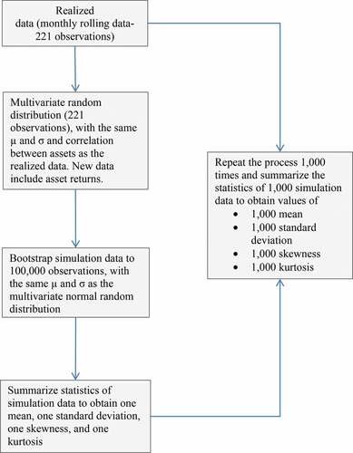
For a one-year simulation, the mean and standard deviation of the monthly returns are calculated. The annual asset correlations are formed from the observed returns of stocks, bonds, bills, commodities, and real estate investment trusts. Next, 12 monthly random observations are drawn with replacement from the base sample in the second step and sum up to 12 monthly random observations to acquire one annual simulated return. Drawing and summing up random observations are repeated until 100,000 annual bootstrapped observations are achieved. Longer horizon returns are treated similarly.

For all horizons, the 100,000 bootstrapped returns are extracted to obtain one mean, one standard deviation, one skewness, and one kurtosis, and then calculate correlations between assets. The drawing of 100,000 simulated returns 1000 times is repeated to acquire 1000 means, 1000 standard deviations, 1000 skewness, and 1000 kurtosis. The moments of correlations for 1000 correlations between assets are obtained.

4. Empirical findings and discussions

4.1. Normal convergence of asset returns

Table 1 summarises the data on the distribution of realized monthly continuously compounded returns and the simulated continuously compounded returns of one replica of the 1,000 simulation runs. Each of the 100,000 continuously compounded returns of T horizon (C_T) returns is a total of T individual draws with the replacement of 221 monthly continuously compounded returns for the period from 1970 to 2018. The central limit theorem implies that the virtual continuously compounded returns achieve normal distributions as the time (T) horizon extends.

Table 1. Speed of convergence to the normal distribution

		1 month	1 year	3 years	5 years	10 years	20 years	30 years
Stocks	Mean	0.009	0.113	0.386	0.651	1.079	2.850	2.984
	SD	0.051	0.161	0.295	0.361	0.543	0.748	0.930
	Skew	−0.226	−0.085	0.070	−0.027	0.004	0.009	−0.016
	Kurt	3.684	3.061	2.988	3.002	3.022	2.956	3.012
	JB	2795.764*	135.022*	82.227*	12.340*	2.252	9.490	5.038
Bonds	Mean	0.005	0.043	0.282	0.330	0.846	2.461	2.590
	SD	0.029	0.090	0.160	0.196	0.298	0.432	0.550
	Skew	−0.105	−0.029	0.001	−0.009	−0.019	−0.011	−0.004
	Kurt	3.063	2.959	3.018	3.011	3.035	3.003	3.018
	JB	200.743*	21.124*	1.374	1.750	11.132	2.192	1.615
Bills	Mean	0.006	0.069	0.219	0.371	0.751	1.508	2.275
	SD	0.002	0.007	0.015	0.017	0.026	0.033	0.042
	Skew	0.433	0.043	−0.009	−0.069	−0.020	−0.023	0.009
	Kurt	3.276	3.022	2.983	2.986	3.007	2.989	2.989
	JB	3438.871*	32.636*	2.480	80.144	6.732	9.552*	1.708
Commodities	Mean	0.005	0.040	−0.006	0.284	0.560	−0.941	−2.126
	SD	0.055	0.173	0.346	0.395	0.599	0.797	1.027
	Skew	0.078	0.059	0.009	0.014	0.008	−0.002	−0.014
	Kurt	3.434	3.008	3.020	2.992	3.007	2.997	2.993
	JB	885.438*	58.290*	2.905	3.475	1.259	0.111	3.305
REITs	Mean	−0.020	−0.111	−0.061	−0.253	−0.392	−1.628	−4.221
	SD	0.083	0.292	0.510	0.631	0.939	1.337	1.556
	Skew	0.117	−0.101	0.000	−0.047	−0.002	0.027	0.022
	Kurt	3.192	3.033	3.000	2.972	3.001	2.982	3.011
	JB	380.422*	175.931*	0.003*	40.468	0.054	13.560*	8.208

This table summarises the averages of one simulation replication (see Appendix Table A3). Following the fixed sample (FS) simulation process of Fama and French (2018), each repetition of simulations generates 100,000 continuously compounded returns for each period by drawing monthly returns from multivariate normal distributions. The mean and standard deviation of observed monthly returns, as well as the correlations between rolling asset returns across investment horizons, are used as distribution inputs. The parameters are for various assets such as stocks, bonds, bills, commodities, and real estate investment trusts. The presented averages of parameters for various assets are the mean, standard deviations (SD), skewness (Skew), and kurtosis (Kurt) of the 100,000 simulated continuously compounded returns. Skew is calculated by dividing the third moment about the mean by SD³. Kurt is defined as the fourth moment about the mean divided by SD⁴. The symbol * reflects the 1% significance amount for the Jarque-Bera (JB) normality test, meaning that the null hypothesis is rejected with a joint hypothesis of skewness and excess kurtosis being zero. REITs stand for real estate investment trusts.

In absolute terms, the realized monthly continuously compounded returns for the 1970–2018 period are either skewed left (stock and bond) or right (other) and leptokurtic. Skewness and kurtosis decay over one year, 10 years, and 30 years across asset classes. Furthermore, when drawn from normal multivariate distributions, the returns converge to normal distributions at a rate other than $1/\sqrt{T}$. Specifically, the skewness for the simulated stock returns, commodity returns, and real estate investment trusts’ returns converge at a faster pace than the expected skewness ($\text{Skewnes}{\mathrm{s}}_{1\mathit{\text{month}}}/\sqrt{T}$ (Fama & French, 2018)) and increases after 10 years.

However, the figures for bond returns and bill returns consistently approach normality at a faster rate than the projected values. In-depth, the simulated (expected) skewness decreases to-0.085 (−0.065) for stock returns, −0.029 (−0.030) for bond returns, 0.043 (0.125) for bill returns, 0.059 (0.224) for commodity returns and −0.101 (0.337) for one year returns for real estate investment trusts. Skewness for 10-year and 30-year horizons is very different across asset classes. Besides, Kurtosis is usually predicted to reach its normal value (3,000) quicker than skewness. Kurtosis in horizons varies from the predicted value, ($\mathit{\text{Kurtosi}}{s}_{1\mathit{\text{month}}}-3.0)/T$, but achieves normality as the horizon extends.

The decay rate of skewness and kurtosis in Table 1 departs from expectations due to sampling errors. The cross-iteration standard deviations of skewness and kurtosis in Appendix Table A2 also decline over horizons at a near-projected decay rate of skewness and kurtosis. This occurs because the iteration skewness in T longer horizons is $\text{Skewnes}{\mathrm{s}}_{1\mathit{\text{month}}}/\sqrt{T}$ coupled with sampling error, and the kurtosis is $(\mathit{\text{Kurtosi}}{s}_{1\mathit{\text{month}}}-3.0)/T$ coupled with the sampling error. In summary, with longer horizons, the standard deviations of skewness and kurtosis from Appendix Table A2 become smaller.

Table 2. Moments of asset payoffs without incorporating the uncertainty about the expected returns

		1 month	1 year	3 years	5 years	10 years	20 years	30 years
Stocks	Mean	1.009	1.102	1.373	1.714	3.058	10.957	46.006
	SD	0.050	0.182	0.408	0.673	1.772	9.700	54.141
	Skew	0.002	0.452	0.890	1.215	1.914	3.333	5.135
	Kurt	2.984	3.352	4.431	5.723	10.143	28.315	69.635
Bonds	Mean	1.007	1.082	1.293	1.542	2.412	6.116	15.643
	SD	0.027	0.098	0.209	0.324	0.730	2.689	8.611
	Skew	0.004	0.246	0.476	0.629	0.927	1.399	1.819
	Kurt	2.959	3.105	3.401	3.707	4.567	6.678	9.423
Bills	Mean	1.006	1.071	1.243	1.442	2.095	4.420	9.294
	SD	0.002	0.008	0.017	0.025	0.052	0.154	0.399
	Skew	0.004	0.022	0.040	0.051	0.074	0.104	0.128
	Kurt	2.973	2.998	3.003	3.004	3.010	3.020	3.029
Commodities	Mean	1.003	1.029	1.097	1.188	1.490	2.590	6.357
	SD	0.055	0.187	0.361	0.516	0.966	2.612	8.769
	Skew	0.002	0.500	0.990	1.356	2.190	4.041	6.703
	Kurt	2.984	3.435	4.779	6.425	12.578	41.812	143.614
REITs	Mean	0.995	0.945	0.858	0.777	0.687	0.680	1.103
	SD	0.084	0.268	0.452	0.556	0.783	1.395	3.678
	Skew	−0.009	0.786	1.660	2.442	4.795	13.291	30.511
	Kurt	2.970	4.085	8.241	15.150	60.286	584.371	2842.457

This table summarises data on 100,000 simulated payoffs derived from 221 realized monthly returns using sampling with replacement. For the 1970–2018 period, the one-month estimates show moments of monthly payoffs (1+realized monthly returns). The parameters given are the mean, standard deviations (SD), skewness (Skew), and kurtosis (Kurt) of 100,000 simulated continuously compounded payoffs for each horizon. Skew is determined by dividing the third moment by the mean by SD³. Kurt is defined as the fourth moment about the mean divided by SD⁴. REITs stand for real estate investment trusts.

The skewness of one distribution replica (Table 1) is not more than three cross-replication standard deviations (Appendix Table A2) from 0.000. The common deviation is between one or two standard deviations from 0.000. Kurtosis values (Table 1) suggest that convergence to normality is not complete for returns on stocks, bonds, and real estate investment trusts because one unexpected deviation from 3,000 (more than five standard deviations) occurs in one of those assets’ returns within 10 years or longer horizons. In conclusion, skewness and kurtosis imply the asset returns revert to normal distributions in a 10-year horizon or longer.

The Jarque-Bera normality test to asset returns at a 1% significance level is applied and finds that convergences to normal return distributions occur after a 10-year investment horizon. Investors must be cautious of the non-normal distributions which may include fat tails and high peaks during the simulation phase. The findings confirm those of previous studies that find a difference in statistical properties between stocks, bonds, and bills and alternative classes such as commodities (Gorton & Rouwenhorst, 2006), real estate (Myer & Webb, 1994), and private equity (Cumming et al., 2013).

4.2. The conclusion for hypothesis 1

Higher moments of returns (Kurtosis and skewness values) and Jarque-Bera test values suggest that the convergence to normality for returns happens after 10 years. For investment horizons of less than 10 years, the null hypothesis is not rejected. The null hypothesis is denied; however, when the investment horizon exceeds 10 years.

4.3. Simulations of asset payoffs

Investors are typically concerned about their payoffs and ignore facts about continuously compounded returns. Table 2 summarises data on realized and virtual continuously compounded return distributions from 1970 to 2018. The table shows the mean, standard deviation, skewness, and kurtosis of the payoffs for each return horizon. The distribution of realized monthly payoffs is analyzed in the one-month lines. Other rows display the distribution of 100,000 bootstrapped payoffs over longer periods.

Empirical findings provide several surprising observations. The payoffs and uncertainty about the payoffs grow as the period T becomes longer. The skewness of payoff distributions also rises, from 0.000 for stocks, 0.004 for bonds, 0.0042 for bills, 0.002 for commodities, and −0.008 for real estate investment trusts for monthly payoffs to 5.135 for stocks, 1.819 for bonds, 0.128 for bills, 6.703 for commodities, and 30.511 for real estate investment trusts for 30-year payoffs. Despite higher estimation errors in payoffs for longer time horizons, the increase in average payoffs and skewness combine to pull the distribution to the right as the time horizon (T) increases. Kurtosis is greater than 3.0 for most horizons; it is marginally less than three for one-month payoffs and rises for longer horizons. Skewness and kurtosis are extreme in the distributions of commodity and real estate investment trusts’ payoffs, but near to normality in the distribution of bill payoffs. The kurtosis of commodity and real estate investment trusts’ payoff distributions rises at an exponential rate, growing from 12.58 (commodity) and 60.29 (real estate investment trusts) in 10 years to 60.29 (commodity) and 2842.46 (real estate investment trusts). In summary, payoff distributions in longer time horizons are becoming leptokurtic, but their increasing positive skewness suggests that outliers still exist in the right tail.

There have been concerns over whether the distribution of payoffs approaches lognormal as investment horizons expand. Since the relation between continuously compounded returns and payoffs is clear, as C_T converges to normality as the time horizon (T) increases, payoffs approximate lognormal. The payoff is calculated as the exponential of 1 + R_T. As a result, the normality convergence rate of returns is the same as the lognormality convergence rate of payoffs. Since the normal convergence of continuously compounded returns is not complete after 10 years, the normal convergence of payoffs is not final.

4.4. Uncertainty about the expected asset returns

Table 3 summarises statistics on asset payoffs that include uncertainty about the expected return. Uncertainty over asset returns has a minor impact on payoff distributions over the short term. The random error increases the standard deviations of simulated three-year returns for the 1970–2018 period from one percent to three percent for the all-assets portfolio.

Table 3. Asset payoffs incorporating the uncertainty about the expected returns

		1 month	1 year	3 years	5 years	10 years	20 years	30 years
Stocks	Mean	1.009	1.100	1.360	1.688	3.005	10.447	40.854
	SD	0.050	0.182	0.408	0.664	1.745	9.318	48.299
	Skew	−0.004	0.454	0.895	1.215	1.918	3.376	5.245
	Kurt	2.953	3.358	4.451	5.718	10.194	28.559	77.743
Bonds	Mean	1.007	1.084	1.291	1.528	2.417	6.149	16.250
	SD	0.027	0.098	0.209	0.320	0.726	2.688	8.894
	Skew	−0.014	0.249	0.475	0.624	0.919	1.393	1.807
	Kurt	2.992	3.105	3.400	3.697	4.538	6.648	9.320
Bills	Mean	1.006	1.070	1.242	1.441	2.090	4.401	9.243
	SD	0.002	0.008	0.017	0.025	0.051	0.153	0.396
	Skew	−0.003	0.023	0.039	0.050	0.073	0.104	0.128
	Kurt	2.982	2.999	3.002	3.003	3.009	3.019	3.029
Commodities	Mean	1.002	1.027	1.097	1.201	1.518	2.658	6.310
	SD	0.054	0.186	0.361	0.521	0.978	2.685	8.673
	Skew	0.006	0.498	0.990	1.351	2.177	4.007	6.530
	Kurt	2.959	3.432	4.777	6.397	12.459	40.873	125.943
REITs	Mean	0.996	0.951	0.870	0.804	0.713	0.902	1.325
	SD	0.084	0.270	0.458	0.572	0.811	1.850	4.213
	Skew	1.000	0.783	1.658	2.423	4.825	13.609	28.773
	Kurt	2.988	4.075	8.215	14.830	64.521	592.814	2422.891

This table summarises statistics from 100,000 simulated payoffs derived from 221 realized monthly returns using sampling with replacement. The parameters shown are mean, standard deviations (SD), skewness (Skew), and kurtosis (Kurt). Skew is determined by dividing the third moment by the mean by SD³. Kurt is defined as the fourth moment about the mean divided by SD⁴. For each 100,000 simulation run, The standard errors taken from normal distributions of errors of mean zero and standard deviations are equal to the standard error of the average realized monthly returns for the 1970–2018 period. The add-in standard errors are 0.19 percent for stock returns, 0.10 percent for bond returns, 0.01 percent for bill returns, 0.24 percent for commodity returns, and 0.30 percent for real estate investment trusts (REITs)’ returns. The one-month figures show moments of the monthly payoffs (1+ realized monthly return).

However, uncertainty regarding average projected returns raises the standard deviations of stock and real estate investment trusts’ payoffs by 12 percent and 13 percent, respectively, over 30-year horizons. The shift in standard deviations of bond, bill, and product returns is negligible. Longer time horizons cause asset payoffs to become right-skewed and kurtoleptic. For example, if the calculation errors of the anticipated return are ignored, the kurtosis of stock payoff distributions at 30-year horizons is 66.64 and 77.74 when random errors are included. Incorporating random errors reduces the kurtosis of commodities and real estate investment trusts by 14 percent and 17 percent, respectively. Uncertainty, on the other hand, has a little major impact on bill and bond payoff distributions. In general, measurement errors of the expected return are an irrelevant source of uncertainty for short-horizon payoffs, but they become important in long-horizon payoffs of stocks, commodities, and real estate investment trusts, but the gap between payoffs with and without errors is negligible for bills and bonds. Our results affirm the findings of Pastor and Stambaugh (2012) and Fama and French (2018) based on their theoretical and methodological approaches.

4.4.1. The conclusion for hypothesis 2

In summary, estimation errors are not pertinent to any causes of short-term investment payoff uncertainty, but they are substantial for long-term asset payoff uncertainty. The minimal effects of estimation errors on the payoff distributions of bonds and bills are an exception to these findings. With the notable exception of bonds and bills, the conclusion of hypothesis 2 is that estimation errors of monthly returns have a substantial impact on the variability of long-horizon asset returns and payoffs.

5. Conclusions

This study employs Fama and French’s (2018) simulation to investigate the stylized facts of long-horizon market returns and portfolio returns. The central limit theorem proposes that the distributions of continuously compounded returns converge to normality as the investment horizon expands. On a purely random basis, the realized monthly continuously compounded returns used as the base for the bootstrap simulations are independent and identically distributed, so they converge toward normal distributions. Variations from normal distributions are large in the short run, but they diminish as the investment horizon increases. For 10 years or longer, kurtosis is indifferent to the value of normality, 3.0. The left-skewed returns (stock returns and bond returns) or the right-skewed returns (bill returns, commodity returns, and real estate investment trusts’ returns) eventually revert to normal (0.0) in longer horizons. Estimations of parameters of continuously compounded returns become more precise in longer investment horizons, and the remaining negative or positive skewness is no more than three standard deviations from zero. The Jarque-Bera normality test at a 1% significance level is applied to asset returns and finds those return distributions converge to normality from the 10-year investment period. Also, the stock return distribution converges at the slowest rate to normality.

Investment payoffs (1+R_T) are a direct conversion of continuously compounded returns (R_T) as they are exponential of continuously compounded returns. However, while the continuously compounded returns eventually approach normality, the payoffs fail to achieve log normality. The study findings strengthen the results of Pastor and Stambaugh (2012), Fama and French (2018), and Madan and Wang (2021). More importantly, the skewness and kurtosis of asset classes provide evidence for the benefits of diversification as the inclusion of different asset classes helps the return distribution converge faster towards normal distributions. Higher stock concentration increases the normal convergence of payoffs, however, at a marginal pace to the normal convergence of the same asset allocations in longer horizons. In addition, including more assets provides higher diversification as it speeds up the normal convergence of payoffs towards lognormal distributions.

Like Pastor and Stambaugh (2012), Fama and French (2018), and Bessembinder (2021), this research finds that uncertainty about the expected returns has a great impact, on the long-horizon payoffs; however, the degree of impact is smaller across higher stock allocation than longer horizons. The estimation errors of monthly expected returns are hindered by the dispersions caused by the unexpected return. The errors, nonetheless, impact the variations of possible payoffs in 10-year (or more) investment periods.

This study offers some important implications for research scholars and practitioners. There are two implications for the academic researcher. First, introducing more assets to the portfolio offers diversification benefits in the long run. Second, this study ameliorates the easy data bias and provides a more accurate description of tail outcomes that are of concern to academic researchers in optimal portfolio selection and asset management, optimized consumption and savings behavioral patterns in life-cycle models, and the evaluation of macroeconomic analysis of asset values. There are two implications for investors. First, investors should evaluate higher moments and the probability and size of severe tail events due to the single-draw nature of long-term returns for pension savers. Second, investors can improve their simulations to examine the distributions of long-horizon payoffs by including the uncertainty about the expected returns in the simulation run.

Disclosure statement

No potential conflict of interest was reported by the author(s).

Additional information

Notes on contributors

Tri M. Hoang

Tri M. Hoang is a lecturer at Vietnam’s HUTECH University. His research interests include behavioral finance and markets, as well as empirical asset pricing

Notes

1. From their analysis, the empirical results of Fama and French (2018) for stock returns are reproduced for the same sampling duration (1963–2016). The findings of our replication are identical to theirs (see Appendix Table A1).

Appendix

Table A1. Averages of 1000 replications using actual and bootstrapped return using the industry-calculated mean and standard deviations

Table

		1 month	1 year	3 years	5 years	10 years	20 years	30 years
Stock returns	Mean	0.009	0.106	0.317	0.528	1.056	2.112	3.168
	SD	0.050	0.173	0.299	0.386	0.546	0.772	0.945
Bond returns	Mean	0.007	0.085	0.256	0.426	0.852	1.704	2.556
	SD	0.027	0.095	0.164	0.212	0.299	0.423	0.518
Bill returns	Mean	0.006	0.074	0.223	0.372	0.744	1.488	2.232
	SD	0.002	0.008	0.014	0.018	0.025	0.036	0.044
Commodity returns	Mean	0.003	0.032	0.097	0.162	0.324	0.648	0.972
	SD	0.055	0.189	0.327	0.422	0.597	0.844	1.034
REITs’ returns	Mean	−0.005	−0.060	−0.180	−0.300	−0.600	−1.200	−1.800
	SD	0.084	0.290	0.502	0.648	0.916	1.295	1.586

This table summarizes the total of 1000 simulation replications. Using the industry’s standard rule of thumb, the averages and standard deviations are summarized for all return horizons. The industry-standard approach for calculating standard deviations from monthly returns for longer time horizons is to multiply the monthly standard deviations by the square root of the time horizon. To determine the mean returns from monthly returns for longer time horizons, the monthly returns are multiplied by the time horizon. REITs stand for real estate investment trusts.

Table A2. Standard deviations of asset return moments

Table

		1 month	1 year	3 years	5 years	10 years	20 years	30 years
Stocks	Mean	0.003	0.037	0.113	0.203	0.390	0.778	1.199
	SD	0.002	0.008	0.014	0.018	0.027	0.036	0.045
	Skew	0.165	0.048	0.029	0.022	0.018	0.013	0.012
	Kurt	0.313	0.033	0.019	0.017	0.016	0.016	0.016
Bonds	Mean	0.002	0.020	0.063	0.109	0.222	0.433	0.655
	SD	0.001	0.004	0.008	0.010	0.014	0.021	0.024
	Skew	0.165	0.051	0.029	0.022	0.018	0.013	0.012
	Kurt	0.299	0.034	0.017	0.016	0.016	0.015	0.015
Bills	Mean	0.000	0.002	0.005	0.009	0.018	0.036	0.056
	SD	0.000	0.000	0.001	0.001	0.001	0.002	0.002
	Skew	0.165	0.049	0.029	0.022	0.016	0.013	0.012
	Kurt	0.321	0.032	0.018	0.017	0.016	0.015	0.015
Commodities	Mean	0.004	0.041	0.127	0.213	0.444	0.840	1.325
	SD	0.003	0.009	0.015	0.020	0.027	0.042	0.048
	Skew	0.163	0.049	0.029	0.022	0.017	0.013	0.011
	Kurt	0.326	0.032	0.019	0.017	0.015	0.016	0.016
REITs	Mean	0.006	0.064	0.186	0.339	0.658	1.355	2.144
	SD	0.004	0.013	0.023	0.031	0.043	0.058	0.076
	Skew	0.162	0.049	0.029	0.021	0.017	0.013	0.011
	Kurt	0.304	0.031	0.018	0.017	0.015	0.015	0.016

This table summarizes the standard deviations of 1000 replications of simulations. Following Fama and French’s (2018) fixed sample simulation method, each replication of simulations constructs 100,000 continuously compounded returns for every horizon by drawing monthly returns from multivariate normal distributions. The distribution inputs are the mean and standard deviation of the realized monthly returns and the correlations between rolling asset returns across investment horizons. This table provides standard deviations of parameters for different assets, including stocks, bonds, bills, commodities, and real estate investment trusts (REITs). The parameters are mean, standard deviations (SD), skewness (Skew), and kurtosis (Kurt) of the 100,000 simulated continuously compounded returns for each horizon. Skew is the third moment about the mean divided by SD³.Kurt is the fourth moment about the mean divided by SD⁴.

Table A3. Averages of 1000 replications using actual and bootstrapped asset returns

Table

		1 month	1 year	3 years	5 years	10 years	20 years	30 years
Stocks	Mean	0.009	0.097	0.312	0.521	1.047	2.111	3.114
	SD	0.050	0.165	0.294	0.383	0.544	0.768	0.945
	Skew	0.002	−0.001	0.001	0.001	0.000	0.000	0.000
	Kurt	2.984	2.996	3.000	3.000	3.000	3.000	3.000
Bonds	Mean	0.007	0.079	0.256	0.429	0.859	1.726	2.550
	SD	0.027	0.091	0.162	0.210	0.298	0.424	0.519
	Skew	0.004	0.000	0.002	0.000	0.000	0.000	0.001
	Kurt	2.959	2.999	2.998	2.999	3.001	3.000	3.001
Bills	Mean	0.006	0.068	0.218	0.367	0.742	1.490	2.235
	SD	0.002	0.008	0.014	0.018	0.025	0.035	0.043
	Skew	0.004	0.001	0.001	−0.001	0.001	0.000	0.000
	Kurt	2.973	2.997	3.000	2.999	3.000	3.001	3.000
Commodities	Mean	0.003	0.028	0.085	0.150	0.302	0.610	0.951
	SD	0.055	0.181	0.322	0.418	0.595	0.843	1.036
	Skew	0.002	0.001	0.001	−0.001	−0.001	0.000	0.000
	Kurt	2.984	2.997	2.999	2.999	3.000	3.000	3.001
REITs	Mean	−0.005	−0.059	−0.170	−0.308	−0.593	−1.258	−1.873
	SD	0.084	0.277	0.494	0.642	0.913	1.288	1.586
	Skew	−0.009	0.001	0.001	0.000	0.000	0.000	−0.001
	Kurt	2.970	2.997	3.000	2.999	3.000	3.000	3.000

This table summarises the averages of 1000 replications of simulations. Following Fama and French’s (2018) simulation method, each replication of simulations constructs 100,000 continuously compounded returns for every horizon by drawing monthly returns from multivariate normal distributions. The distribution inputs are the mean and standard deviation of the realized monthly returns and the correlations between rolling asset returns across investment horizons. This table provides averages of parameters for different assets, including stocks, bonds, bills, commodities, and real estate investment trusts (REITs). The parameters are mean, standard deviations (SD), skewness (Skew), and kurtosis (Kurt) of the 100,000 simulated continuously compounded returns for each horizon. Skew is the third moment about the mean divided by SD³. Kurt is the fourth moment about the mean divided by SD⁴.

References

- Anarkulova, A., Cederburg, S., & O’Doherty, M. S. (2022). Stocks for the long run? Evidence from a broad sample of developed markets. Journal of Financial Economics, 143(1), 409–16. https://doi.org/10.1016/j.jfineco.2021.06.040
- Ang, A., Papanikolaou, D., & Westerfield, M. (2014). Portfolio choice with illiquid assets. Management Science, 60(11), 2737–2761. https://doi.org/10.1287/mnsc.2014.1986
- Arditti, F. D., & Levy, H. (1975). Portfolio efficiency analysis in three moments: The multiperiod case†. The Journal of Finance, 30(3), 797–809. https://doi.org/10.1111/j.1540-6261.1975.tb01851.x
- Avramov, D., Cederburg, S., & Lučivjanská, K. (2018). Are stocks riskier over the long run? Taking cues from economic theory. The Review of Financial Studies, 31(2), 556–594. https://doi.org/10.1093/rfs/hhx079
- Bachelier, L. J. B. A. (1914). Le Jeu, la chance, et le hasar. Ernest Flammarion.
- Bessembinder, H. (2018). Do stocks outperform Treasury bills? Journal of Financial Economics, 129(3), 440–457. https://doi.org/10.1016/j.jfineco.2018.06.004
- Bessembinder, H. (2021). Wealth Creation in the US Public Stock Markets 1926–2019. Journal of Investing, 30(3), 47–61. https://doi.org/10.3905/joi.2021.1.168
- Carvalho, C. M., Lopes, H. F., & McCulloch, R. E. (2018). On the long-run volatility of stocks. Journal of the American Statistical Association, 113(523), 1050–1069. https://doi.org/10.1080/01621459.2017.1407769
- Chun, G. H., Sa-Aadu, J., & Shilling, J. D. (2004). The role of real estate in an institutional investor’s portfolio revisited [journal article]. The Journal of Real Estate Finance & Economics, 29(3), 295–320. https://doi.org/10.1023/b:Real.0000036675.46796.21
- Cumming, D., Helge Haß, L., & Schweizer, D. (2013). Private equity benchmarks and portfolio optimization. Journal of Banking & Finance, 37(9), 3515–3528. https://doi.org/10.1016/j.jbankfin.2013.04.010
- Dahlquist, M., Farago, A., & Tédongap, R. (2016). Asymmetries and Portfolio Choice. The Review of Financial Studies, 30(2), 667–702. https://doi.org/10.1093/rfs/hhw091
- Diris, B., Palm, F., & Schotman, P. (2015). Long-term strategic asset allocation: An out-of-sample evaluation. Management Science, 61(9), 2185–2202. https://doi.org/10.1287/mnsc.2014.1924
- Fama, E. (1965a). The behavior of stock-market prices. The Journal of Business, 38(1), 34–105. https://doi.org/10.1086/294743
- Fama, E. (1965b). Random walks in stock market prices. Financial Analysts Journal, 21(5), 55–59. https://doi.org/10.2469/faj.v21.n5.55
- Fama, E., & French, K. (2018). Long-horizon returns. The Review of Asset Pricing Studies, 8(2), 232–252. https://doi.org/10.1093/rapstu/ray001
- Gorton, G., & Rouwenhorst, K. G. (2006). Facts and fantasies about commodity futures. Financial Analysts Journal, 62(2), 47–68. https://doi.org/10.2469/faj.v62.n2.4083
- Huang, J., & Zhong, Z. (2011). Time variation in diversification benefits of commodity, reits, and tips. The Journal of Real Estate Finance & Economics, 46(1), 152–192. https://doi.org/10.1007/s11146-011-9311-6
- Jurczenko, E., Maillet, B., & Merlin, P. (2012). Hedge fund portfolio selection with higher-order moments: a nonparametric mean-variance–skewness–kurtosis efficient frontier multi‐moment asset allocation and pricing models. https://doi.org/10.1002/9781119201830.ch3
- Kan, R., & Zhou, G. (2007). Optimal portfolio choice with parameter uncertainty. The Journal of Financial and Quantitative Analysis, 42(3), 621–656. https://doi.org/10.1017/S0022109000004129
- Kendall, M. G. (1948). The advanced theory of statistics. C. Griffin & Co.
- Kothari, S. P., & Shanken, J. (2004). Asset allocation with inflation-protected bonds. Financial Analysts Journal, 60(1), 54–70. https://doi.org/10.2469/faj.v60.n1.2592
- Lusinski, N. (2018). 7 Tips to Help Make Saving for Retirement Easier, According to a Financial Planner. Insider Inc. Retrieved July 6, 2020 from https://www.businessinsider.com/retirement-tips-from-a-financial-planner-2018-10#7-dont-underestimate-healthcare-costs-in-retirement-7
- Madan, D. B., & Schoutens, W. (2020). Self-similarity in long-horizon returns. Mathematical Finance, 30(4), 1368–1391. https://doi.org/10.1111/mafi.12269
- Madan, D. B., & Wang, K. (2021). The structure of financial returns. Finance Research Letters, 40(3), 1572–1616. https://doi.org/10.1016/j.frl.2020.101665. 101665.
- Michaud, R., & Michaud, R. (2008). Efficient asset management: A practical guide to stock portfolio optimization and asset allocation (2nd ed.). Oxford University Press.
- Mitton, T., & Vorkink, K. (2007). Equilibrium underdiversification and the preference for skewness. Review of Financial Studies, 20(4), 1255–1288. https://doi.org/10.1093/revfin/hhm011
- Myer, N., & Webb, J. (1994). Statistical properties of returns: Financial assets versus commercial real estate [journal article]. The Journal of Real Estate Finance & Economics, 8(3), 267–282. https://doi.org/10.1007/bf01096997
- Ndiaye, D. A. (2019). Asset return determinants: risk factors, asymmetry and horizon consideration [ Dissertation, Université de Lyon].
- Neuberger, A., Payne, R., & Van Nieuwerburgh, S. (2021). The skewness of the stock market over long horizons. The Review of Financial Studies, 34(3), 1572–1616. https://doi.org/10.1093/rfs/hhaa048
- Osborne, M. F. M. (1959). Brownian motion in the stock market. Operations Research, 7(2), 145–173. https://doi.org/10.1287/opre.7.2.145
- Pastor, L., & Stambaugh, R. (2012). Are stocks less volatile in the long run? Journal of Finance, 67(2), 431–478. https://doi.org/10.1111/j.1540-6261.2012.01722.x
- Phillips, B. (2016). A pension plan for the creative class. The New York Times Company. Retrieved October 15, 2018 from https://www.nytimes.com/2016/03/06/business/retirementspecial/a-pension-plan-for-the-creative-class.html?ref=retirementspecial
- Platanakis, E., Sakkas, A., & Sutcliffe, C. (2018). Harmful diversification: Evidence from alternative investments. The British Accounting Review, 51(1), 1–23. https://doi.org/10.1016/j.bar.2018.08.003
- Roll, R. (2004). Empirical tips. Financial Analysts Journal, 60(1), 31–53. https://doi.org/10.2469/faj.v60.n1.2591
- Sa-Aadu, J., Shilling, J., & Tiwari, A. (2010). On the portfolio properties of real estate in good times and bad times1. Real Estate Economics, 38(3), 529–565. https://doi.org/10.1111/j.1540-6229.2010.00276.x