Quantifying systemic risk in Morocco’s banking system using Euler indicators and extreme dependence

Abstract

This article contributes to the quantification of systemic risk within the Moroccan banking system, focusing on listed banks. We utilize indicators derived from Tail Value at Risk and expectiles risk measures, as introduced by El qalli and Said (2013) (El Qalli & Said, 2023), to measure the marginal risk of each component. Additionally, we analyze extreme dependencies within the system using tail dependence coefficients. Empirical results identify Attijariwafa Bank and Banque Centrale Populaire as the most systemic banks in Morocco, carrying the potential to trigger systemic crises.

Keywords:

• Systemic risk
• risk measures
• Euler Method
• extreme dependence
• Copulas

JEL classification:

• C02
• G01
• G21
• G28
• G32

1. Introduction

In a world grappling with sustained inflation and economic recession risks, the stability of banking systems faces serious threats. Recent events, including the crisis among regional American banks in March 2023, UBS’s acquisition of Credit Suisse, and JPMorgan’s takeover of First Republic Bank, highlight the urgency of addressing systemic risk.

Panic spreads swiftly, increasing contagion risks with each bank collapse, as seen in the recent collapse of three American regional banks. The US government responded with swift measures to halt panic, guaranteeing deposits and implementing the Bank Term Funding Program. Europe also faced systemic risk, with Credit Suisse’s near collapse affecting other European banks, emphasizing the need for systemic risk management.

Despite progress with Basel III, systemic risk remains a challenge. Rapid regulatory reactions have prevented the worst, but concerns persist. Resolving crises through mergers can create uncontrollable giants, raising future disaster risks. Deposit guarantees reassure clients but do not fully control panic risk.

In Morocco, the banking system comprises 19 banks, with only 6 listed on the Casablanca Stock Exchange. The central bank increased interest rates to curb inflation, testing Moroccan banks’ risk management. As financial regulators in Morocco draw inspiration from international risk management practices, it becomes paramount to assess and quantify systemic risk within the Moroccan banking system.

This article aims to quantify systemic risk within Morocco’s banking system, focusing on listed banks. We acknowledge market inefficiency due to low liquidity but employ a dependence-based approach to quantify risk.

The article is divided into four distinct sections. The first section is dedicated to the literature review, presenting various measures of systemic risk discussed in works on risk management. The second section explains the methodology adopted for this study in detail. The third section focuses on the presentation and analysis of the data used to obtain the results, which will then be presented and discussed in the fourth and final section.

1.1. Literature review

Since the last global financial crisis, the significance of systemic risk in finance has grown considerably. The subprime financial crisis underscored the importance of enhancing our comprehension and modeling of systemic risk. Financial institutions are deemed systemically risky if their bankruptcy could harm the entire financial system. Several systemic risk measures have been suggested in the literature since the last financial crisis, and a bulk of academic works was dedicated to evaluating this risk in different contexts.

Acharya et al. (2010) (Acharya et al., 2010) introduced the marginal expected shortfall (MES) as a measure of systemic risk. It is denoted as $MES$ and defined mathematically for two random variables representing two risks $X$ and $Y$ by:

$ME{S}_{\alpha }(Y|X)=\mathbb{E}[Y|X\ge Va{R}_{\alpha }(X)],$

where $VaR$ (Value at Risk) is a risk measure of a random variable $X$ at the confidence level $\alpha$:

$Va{R}_{\alpha }(X)=F_X^{-1}(\alpha ):=inf\{x\in \mathbb{R}|F_X(x)\ge \alpha \},$

with $F_X$ being the distribution function of $X$.

Another approach to MES was presented by Acharya et al. (2012) (Acharya et al., 2012), as well as in Acharya et al. (2017) (Acharya et al., 2017). They introduce an economic model of systemic risk, where the overall undercapitalization of the financial sector adversely affects the real economy, leading to systemic risk externality. To measure each financial institution’s contribution to systemic risk, they use the systemic expected shortfall (SES), which indicates the likelihood of an institution being undercapitalized during overall undercapitalization of the financial system. The SES increases based on the institution’s leverage and its marginal expected shortfall (MES), reflecting its losses in the tail of the system’s loss distribution.

Brownlees and Engle (2012) (Brownlees et al., 2012) focused on monitoring a financial system comprising $d$ financial institutions, using the capital shortfall defined as

$C{S}_{it}=k{A}_{it}-W_{it}=k(D_{it}+W_{it})-W_{it},$

as a measure of a firm’s distress. Here, $W_{it}$ represents the market value of equity, $D_{it}$ is the book value of debt, $A_{it}$ is the value of quasi assets, and $k$ is the prudential capital fraction.

To predict the capital shortfall during a systemic event, defined as a market decline below a threshold $C$ over a time horizon $h$, they introduce the SRISK index ($SRIS{K}_{it}$), which represents the expected capital shortfall conditional on a systemic event:

$SRIS{K}_{it}=k{D}_{it}-(1-k)W_{it}(1-LRME{S}_{it}),$

where $LRME{S}_{it}$ is the Long Run MES, representing the expectation of the firm’s equity multi-period arithmetic return during the systemic event, calculated as

$LRME{S}_{it}=-{\mathbb{E}}_t[R_{it+1:t+h}|R_{mt+1:t+h}<C],$

where $R_{it+1:t+h}$ and $R_{mt+1:t+h}$ are respectively the multi-period arithmetic firm equity and market returns between period $t+1$ and $t+h$. Thus, the SRISK index provides a measure of systemic risk for individual financial institutions during potential systemic events.

Adrian and Brunnermeier (2011) (Adrian & Brunnermeier, 2011) propose a metric to assess systemic risk: CoVaR, which calculates the financial system’s Value at Risk (VaR) under distressed conditions of institutions. They measure an institution’s impact on systemic risk by comparing its CoVaR under distress to the CoVaR in a typical state. Through their analysis of publicly traded financial institutions, they evaluate how factors like leverage, size, and maturity mismatch can indicate an institution’s contribution to systemic risk.

This measure, also studied in Adrian and Brunnermeier (2016) (Adrian & Brunnermeier, 2016), is mathematically defined for two random variables $X$ and $Y$, representing the risk of two institutions or an institution and the financial system as follows:

$\mathrm{\Delta }CoVa{R}_{\alpha ,\beta }(Y|X)=CoVa{R}_{\alpha ,\beta }^{=}(Y|X)-Va{R}_{\beta }(Y),$

where

$CoVa{R}_{\alpha ,\beta }^{=}(Y|X)=Va{R}_{\beta }(Y|X=Va{R}_{\alpha }(X)).$

Mainik and Schaanning (2014) (Mainik & Schaanning, 2014) provided explicit formulas for $\mathrm{\Delta }CoVaR$ in particular cases and presented a new approach to this risk measure that takes into account the dependence between risks. This measure was also studied in Löffler and Raupach (2013) (Löffler & Raupach, 2013) and Castro and Ferrari (2014) (Castro & Ferrari, 2014).

Similarly, Mainik and Schaanning (2014) (Mainik & Schaanning, 2014) defined the Conditional Expected Shortfall (CoES), based on the definition of the Expected Shortfall risk measure:

$E{S}_{\alpha }(X)=\frac{1}{1-\alpha }{\int }_{\alpha }^{1}Va{R}_u(X)du.$

The CoES is defined as:

$CoE{S}_{\alpha ,\beta }^{=}(Y|X)=\frac{1}{1-\beta }{\int }_{\beta }^{1}CoVa{R}_{\alpha ,u}^{=}(X)du.$

A second version is given by:

$CoE{S}_{\alpha ,\beta }(Y|X)=\frac{1}{1-\beta }{\int }_{\beta }^{1}CoVa{R}_{\alpha ,u}(X)du,$

where

$CoVa{R}_{\alpha ,\beta }(Y|X)=Va{R}_{\beta }(Y|X\ge Va{R}_{\alpha }(X)).$

Other measures based on financial constructions have been introduced in the literature. For example, the tail risk gamma, presented by Knaup and Wagner (2012) (Knaup & Wagner, 2012), utilizes the sensitivity of an institution’s equity return to changes in put options on system prices.

Recently, El qalli and Said (2013) (El Qalli & Said, 2023) introduced some systemic risk indicators based on capital allocation methods used in actuarial practices. They define, for any positive homogeneous risk measure $\rho$, the Euler systemic risk indicator by

(1) $SR{I}_{\rho }^{Euler}(X_i|S)=\frac{\rho (X_i)}{\sum _{\mathrm{\ell }=1}^d\rho \left(X_{\mathrm{\ell }}\right)}-\underset{h\to 0}{lim}\frac{\rho \left(\sum _{\mathrm{\ell }=1}^d{X}_{\mathrm{\ell }}\right)-\rho \left(\sum _{\mathrm{\ell }=1}^d{X}_{\mathrm{\ell }}-h{X}_i\right)}{\rho \left(\sum _{\mathrm{\ell }=1}^d{X}_{\mathrm{\ell }}\right)h}$(1)

where $\mathbf{X}=\left(X_1,\dots ,X_d\right)$ is a random risk vector, and $S={\sum }_{k=1}^n{X}_k$. The constructed indicators verify

$SR{I}_{\rho }^{Euler}(X_i|S)\in [-1,1],$

and the institution represented by $X_i$ is considered as systemic in a financial system represented by $S$ when the value of its indicator is negative.

The main idea behind the construction of these indicators is to evaluate systemic risk by quantifying the difference between the marginal risk contribution of a component within the entire system, without considering diversification, and its actual participation in the overall risk obtained using the Euler method of risk allocation. Additionally, in (El Qalli & Said, 2023), other indicators based on the Shapley method and various risk allocation techniques are also presented.

In the context of Morocco, few studies have quantified systemic risk in the banking system. Firano (2015) (Firano, 2015) evaluates this risk using two approaches: conditional value at risk for measuring systemic importance and heteroscedasticity models to assess correlations with the financial system. The paper identifies three banks as the most systemic, with the potential to trigger crises. It introduces a systemic risk index and develops a macro-financial model demonstrating procyclical systemic risk contagion. Nechba (2021) (NECHBA, 2021) studies systemic risk exposure of Moroccan banks for the period 2005–2017, using CoVaR, MES, and SRISK measures. More recently, Kyoud et al. (2023) (Kyoud et al., 2023) analyze the Moroccan banking system’s systemic risk during the COVID-19 crisis using QRNN (Quantile Regression Neural Network) and CoVaR. They find a significant increase in systemic risk due to pandemic-induced market conditions, resulting in higher non-performing loans and reduced asset values.

In this article, our focus lies on the indicators developed by El qalli and Said (2013) (El Qalli & Said, 2023), which employ the Euler method for capital allocation. Specifically, we utilize Euler indicators derived from common risk measures, such as Tail Value at Risk and Expectiles. In order to rank different banks according to their impact on the overall system, we quantify extreme dependence using the coefficients of tail dependence presented in Joe’s study (1997) (Joe, 1997). These coefficients will be calculated based on estimates of dependence structures using copulas.

1.2. Methodology suggested

Let $P_{i,t}$ denote the price of asset $i$ at time $t$. We consider daily log-returns, which can be expressed as follows:

$R_{i,t}=log\left(\frac{P_{i,t}}{P_{i,t-1}}\right).$

We use actuarial notation, which treats risky scenarios as positive variables. Therefore, we define:

$X_{i,t}=-{\alpha }_{i,t}{R}_{i,t},$

where

${\alpha }_{i,t}=\frac{n_i{P}_{i,t}}{{\sum }_{k=1}^6{n}_k{P}_{k,t}},$

with $n_k$ representing the total number of shares of Bank $k$. Thus, ${\alpha }_{i,t}$ corresponds to the weight of Bank $i$ in the system composed of these six banks. For the sake of simplicity and without losing generality, the number of shares for each of the six banks is considered fixed based on the values observed on 19 May 2023. The risk associated with the financial system composed of these six banks, denoted as $S$, is expressed as:

$S_t=\sum _{i=1}^6{X}_{i,t}=-\sum _{i=1}^6{\alpha }_{i,t}{R}_{i,t}=-R_{S,t}.$

We denote $S_{-i}$:

$S_{-i,t}=-\sum _{k=1,i\ne i}^6\frac{n_k{P}_{k,t}}{{\sum }_{\mathrm{\ell }=1,\mathrm{\ell }\ne i}^6{n}_{\mathrm{\ell }}{P}_{\mathrm{\ell },t}}{R}_{i,t},$

which represents the financial system without the bank $i$

1.3. Systemic risk index

We first propose the construction of a straightforward systemic risk index that quantifies a bank’s capacity to contribute to a substantial loss for the entire system. To achieve this, we concentrate on analyzing the extreme dependence between a bank’s losses and those of the overall system. Mathematically, we model this dependence using the coefficient of tail dependence between $-R_i$ (bank’s losses) and $-R_S$ (system’s losses).

We recall the definition of the upper tail dependence coefficient as presented in Joe (1997) (Joe, 1997) for bivariate random variables $(X,Y)$ with continuous marginal distributions:

${\lambda }_U=\underset{u\to 1^{-}}{lim}\mathbb{P}(Y>F_Y^{-1}(u)|X>F_X^{-1}(u)),$

when the limit exists.

The coefficient ${\lambda }_U$ does not depend on the marginal distributions of the risks but rather on their dependence structure. To isolate this structure, we resort to copulas. Recall that Sklar’s theorem (1959) (Sklar, 1959) states the existence and uniqueness of a copula $C:[0,1{]}^2\to [0,1]$ for any pair of continuous random variables $(X,Y)$, satisfying

$\mathbb{P}\left(X\le x,Y\le y\right)=C\left(F_X(x),F_Y(y)\right),\mathrm{\forall }(x,y)\in {\mathbb{R}}^2.$

The coefficient ${\lambda }_U$ can thus be expressed in terms of $C$ as follows:

${\lambda }_U=\underset{u\to 1^{-}}{lim}\frac{1-2u+C(u,u)}{1-u},$

when the limit exists.

The main advantage of this approach is to capture non-linear extreme dependencies without making assumptions on the marginal distributions of log-returns.

We focus on estimating copulas using families of usual parametric copulas and their survival copulas. The survival copula $\bar{C}$ is defined as:

$\mathbb{P}(X\ge x,Y\ge y)=\bar{C}({\bar{F}}_X(x),{\bar{F}}_Y(y)),\mathrm{\forall }(x,y)\in {\mathbb{R}}^2,$

where ${\bar{F}}_X$ and ${\bar{F}}_Y$ are the survival distribution functions of $X$ and $Y$ respectively. $\bar{C}$ is related to $C$ through the following relation:

$\bar{C}(u,v)=u+v-1+C(1-u,1-v),\mathrm{\forall }(u,v)\in [0,1{]}^2.$

The upper tail dependence coefficient of $\bar{C}$ can be expressed as follows:

${\lambda }_U(\bar{C})=\underset{u\to 1^{-}}{lim}\frac{1-2u+\bar{C}(u,u)}{1-u}=\underset{u\to 1^{-}}{lim}\frac{C(1-u,1-u)}{1-u}=\underset{u\to 0^{+}}{lim}\frac{C(u,u)}{u},$

and this expression represents the lower tail dependence coefficient of $C$, defined by:

${\lambda }_L=\underset{u\to 0^{+}}{lim}\mathbb{P}(Y\le F_Y^{-1}(u)|X\le F_X^{-1}(u))=\underset{u\to 0^{+}}{lim}\frac{C(u,u)}{u},$

if the limit exists.

To estimate the coefficients ${\lambda }_U$, we will first estimate the copulas for the pairs $(-R_i,-R_S)$. We will use the semi-parametric Canonical Maximum Likelihood method introduced by Oakes (1994) (Oakes, 1994) to estimate these copulas using empirical marginal distribution functions. The families of estimated copulas are presented in Table 1. We will select the most suitable copula using the Akaike Information Criteria (AIC) as the selection criterion. Finally, we will use the analytical expressions, presented in Table 2, to estimate the corresponding ${\lambda }_U$ coefficients for the selected copulas. Other statistical methods for estimating the tail-dependence coefficient are also presented in the study by Frahm (2005) (Frahm et al., 2005).

Table 1. Evaluated copula families

Copula	$\mathbf{C}$
Independence	$C(u,v)=uv$
Gumbel	$C(u,v)=exp(-((-logu{)}^{\theta }+(-logv{)}^{\theta }{)}^{1/\theta }),\theta \ge 1$.
Frank	$C(u,v)=\frac{-1}{\theta }log\left(1+\frac{(e^{-\theta u}-1)(e^{-\theta v}-1)}{e^{-\theta }-1}\right),\theta \ne 0$.
Clayton	$C(u,v)={\left(u^{-\theta }+v^{-\theta }-1\right)}^{-1/\theta }\theta >0$.
Gaussian	$C_{\rho }(u,v)=\frac{1}{2\pi \sqrt{1-{\rho }^2}}{\int }_{-\mathrm{\infty }}^{{\mathrm{\Phi }}^{-1}(u)}{\int }_{-\mathrm{\infty }}^{{\mathrm{\Phi }}^{-1}(v)}exp\left(\frac{x^2-2\rho xy+y^2}{2(1-{\rho }^2)}\right)dxdy.$
Student	$C_{\rho ,\nu }(u,u)={\int }_{-\mathrm{\infty }}^{{\mathbf{t}}_{\nu }^{-1}(u)}{\int }_{-\mathrm{\infty }}^{{\mathbf{t}}_{\nu }^{-1}(v)}\frac{1}{\pi \nu \sqrt{1-{\rho }^2}}\frac{\mathrm{\Gamma }\left(\frac{\nu }{2}+1\right)}{\mathrm{\Gamma }\left(\frac{\nu }{2}\right)}{\left(1+\frac{x^2-2\rho xy+y^2}{\nu (1-{\rho }^2)}\right)}^{-\frac{\nu }{2}+1}dxdy.$

Table 2. Tail dependence coefficients

Copula	${\lambda }_{\mathbf{U}}$	${\lambda }_{\mathbf{L}}$
Independence	0	0
Gumbel	0	$2-2^{\frac{1}{\theta }}$
Frank	0	0
Clayton	$2^{-\frac{1}{\theta }}$	0
Gaussian	$11_{\{\rho =1\}}$	$11_{\{\rho =1\}}$
$\mathbf{t}\mathbf{(}\rho ,\nu \mathbf{)}$	$\left(2-2{\mathbf{t}}_{\nu +1}\left(\sqrt{\left(\frac{(\nu +1)(1-\rho )}{1+\rho }\right)}\right)\right)11_{\{\rho >-1\}}$	$\left(2-2{\mathbf{t}}_{\nu +1}\left(\sqrt{\left(\frac{(\nu +1)(1-\rho )}{1+\rho }\right)}\right)\right)11_{\{\rho >-1\}}$

To disentangle the extreme dependence from the influence of a bank’s weight on the entire system, we additionally estimate the upper tail dependence coefficient between each bank and the system constituted by the other banks. This process involves following the same steps and employing the same estimation methods used earlier to measure the extreme dependence between the losses of an individual bank $-R_i$ and the system $S_{-i}$.

1.4. Euler systemic risk indicators

The utilization of extreme dependence coefficients offers an initial means to quantify the influence of individual components within the banking system when confronted with extreme loss scenarios. However, these coefficients do not provide a comprehensive understanding of the actual contribution of each component to the aggregated risk of the system. In response to this requirement, we also incorporate the Euler systemic risk indicators ($SR{I}^{Euler}$) as defined in (El Qalli & Said, 2023). These indicators enable us to assess the systemic significance of each component within the system.

From 1, one can derive an indicator from any positive homogeneous risk measure. For the VaR risk measure the indicator is given by:

$SR{I}_{Va{R}_{\alpha }}(X_i|S)=\frac{Va{R}_{\alpha }(X_i)}{\sum _{\mathrm{\ell }=1}^{d}Va{R}_{\alpha }\left(X_{\mathrm{\ell }}\right)}-\frac{\mathbb{E}[X_i|S=Va{R}_{\alpha }(S)]}{Va{R}_{\alpha }(S)}.$

An other generalization presented in (El Qalli & Said, 2023) derived indicators from Wang’s risk measures introduced in (Wang, 2000), and defined as:

$\rho (X)={\int }_0^{1}Va{R}_{\alpha }(X)\mathrm{d}\mathrm{g}(\alpha ),$

where $g$ is an increasing distortion function satisfying $g(0)=0$ and $g(1)=1$. These measures are homogeneous, translation-invariant, and monotone. The systemic risk indicator in this case is given by

(2) $SR{I}_g(X_i|S)=\frac{{\int }_0^{1}Va{R}_{\alpha }(X_i)\mathrm{d}\mathrm{g}(\alpha )}{{\int }_0^1{\sum }_{k=1}^{d}Va{R}_{\alpha }(X_k)\mathrm{d}\mathrm{g}(\alpha )}-\frac{{\int }_0^1\mathbb{E}[X_i|S=Va{R}_{\alpha }(S)]\mathrm{d}\mathrm{g}(\alpha )}{{\int }_0^{1}Va{R}_{\alpha }(S)\mathrm{d}\mathrm{g}(\alpha )},$(2)

where $g$ is the distortion function associated with $\rho$.

In this paper, we center our attention on Euler indicators derived from two widely adopted risk measures: TVaR (Tail Value at Risk) and expectiles. The selection of these measures is well-justified by their coherence properties. Unlike VaR, which lacks sub-additivity, TVaR adheres to the coherence axiom introduced by Artzner et al. (1999) (Artzner et al., 1999). Expectiles also exhibit coherence as risk measures when considering thresholds greater than 0.5. Moreover, they possess the additional advantage of being elicitable, which allows for direct backtesting. Furthermore, expectiles take into account both tails of the distribution when assessing risk.

1.4.1. The TVaR-based systemic risk indicator

The TVaR at level $\alpha$ is defined as the mean of the VaRs that exceed $Va{R}_{\alpha }(X)$:

$TVa{R}_{\alpha }(X)=\frac{1}{1-\alpha }{\int }_{\alpha }^{1}Va{R}_{\mu }(X)\mathrm{d}\mu .$

It is a risk measure belonging to the Wang family and is associated with the following distortion function:

$g_{\alpha }(x)=\frac{x-\alpha }{1-\alpha }11_{\{x\in [\alpha ,1]\}}.$

Note that for a fixed $\alpha \in [0,1]$, $g_{\alpha }$ represents the uniform distribution function with support $[\alpha ,1]$. Hence, we can use (2.1) to derive the expression of the TVaR-based systemic risk indicator. The TVaR systemic risk indicator for $(X_i{)}_{i=1,\dots ,d}$ is given by:

$SR{I}_{TVa{R}_{\alpha }}(X_i|S)=\frac{\mathbb{E}[X_i|X_i\ge Va{R}_{\alpha }(X_i)]}{{\sum }_{k=1}^d\mathbb{E}[X_k|X_k\ge Va{R}_{\alpha }(X_k)]}-\frac{\mathbb{E}[X_i|S\ge Va{R}_{\alpha }(S)]}{\mathbb{E}[S|S\ge Va{R}_{\alpha }(S)]}.$

In the Gaussian case, the explicit expression of this indicator in terms of volatilities and correlations can be readily obtained, thanks to the properties of Gaussian vectors. A similar approach can be extended to the case of a random vector following a Student’s t-distribution. However, to maintain a non-parametric stance and avoid assumptions about the distributions of risks, we refrain from adopting specific distributional assumptions in this article.

Instead, we employ standard statistical estimators to calculate all the expectations involved in the indicator’s expression and the quantile representing the VaR for each risk. The estimation of the indicator can be conducted either statically, considering the entire data period, or dynamically, with a rolling approach over a shorter period. This allows us to capture the dynamics of systemic risk over time without imposing restrictive distributional assumptions on the underlying risks.

The TVaR is a highly effective tail measure for quantifying the risk of losses beyond its threshold. However, it has two minor disadvantages that may introduce bias in risk management decisions based on its value. The first drawback concerns its non-elicitable nature, which means that it cannot be directly backtestable. Let us recall the definition of elicitability presented in Bellini et al. (2015) (Bellini & Bignozzi, 2015). A risk measure $\rho$ is considered elicitable with respect to the class $\mathcal{P}$ if there exists a scoring function $S:{\mathbb{R}}^2\to {\mathbb{R}}^{+}$ such that

$\rho (\mathbb{P})=\underset{x\in \mathbb{R}}{argmin}\int S(x,y)d\mathbb{P}(y),\mathrm{\forall }\mathbb{P}\in \mathcal{P}.$

Elicitability is a desirable statistical property for risk measures. However, in the case of TVaR, its non-elicitable nature is not critical since we can test TVaR using VaR, which is elicitable.

The second point concerns its use in capital allocation, which may penalize risks that perform well in positive scenarios. This is due to its construction, as it measures only one tail of the distribution. These two disadvantages are absent in the case of expectile risk measures. Expectiles are the only risk measures that are both coherent and elicitable, as shown by Bellini and Bignozzi (2015) (Bellini & Bignozzi, 2015), and their economic interpretation integrates both the risk behavior in positive and adverse scenarios. From this perspective, it would be interesting to examine the systemic risk indicator derived from expectile measures.

1.4.2. The expectile-based systemic risk indicator

Expectiles were initially introduced within the context of statistical regression models by Newey and Powell (1987) (Newey & Powell, 1987). For a random variable $X$ with a finite second-order moment, the expectile of level $\alpha$ is defined as follows:

(3) $e_{\alpha }(X)=arg\underset{x\in \mathbb{R}}{min}\mathbb{E}[\alpha (X-x{)}_{+}^2+(1-\alpha )(x-X{)}_{+}^2],$(3)

where $(x{)}_{+}=max(x,0)$. Expectile risk measures are elicitable by construction and are coherent for all $\alpha 1/2$. However, for $\alpha <1/2$, expectiles become super-additive, which makes them incoherent. Notably, when $\alpha =1/2$, the expectile corresponds to the mean value. Throughout this paper, we focus on the case where $\alpha >1/2$.

Alternatively, the expectile can be defined for any random variable with a finite first-order moment as the unique solution of the following equation:

(4) $\alpha \mathbb{E}[(X-x{)}_{+}]=(1-\alpha )\mathbb{E}[(x-X{)}_{+}].$(4)

This equation arises as an optimality condition using the strict convexity of the scoring function. It can also be expressed as:

$\frac{1-\alpha }{\alpha }=\frac{\mathbb{E}[(X-x{)}_{+}]}{\mathbb{E}[(x-X{)}_{+}]}.$

From this definition, we can provide an economic interpretation for the expectile risk measure as a threshold that represents a profits/losses ratio of value $\frac{1-\alpha }{\alpha }$.

The properties of expectile risk measures have been studied in several papers. Interested readers can refer to (Emmer et al., 2015) and (Bellini & DiBernardino, 2017) for more information. A multivariate extension of expectiles is proposed in (Maume-Deschamps et al., 2017), and their asymptotic behavior is studied in (Maume-Deschamps et al., 2018). The Expectile-based capital allocation is examined in (Emmer et al., 2015) and (Said, 2023).

The Expectile-based systemic risk indicator of $(X_i{)}_{i=1,\dots ,6}$ is defined as follows:

(5) $SR{I}_{e_{\alpha }}(X_i|S)=\frac{e_{\alpha }(X_i)}{{\sum }_{k=1}^d{e}_{\alpha }(X_k)}-\frac{\alpha \mathbb{E}\left[X_{i}11_{\{S>e_{\alpha }(S)\}}\right]+(1-\alpha )\mathbb{E}\left[X_{i}11_{\{S<e_{\alpha }(S)\}}\right]}{\alpha \mathbb{E}\left[S11_{\{S>e_{\alpha }(S)\}}\right]+(1-\alpha )\mathbb{E}\left[S11_{\{S<e_{\alpha }(S)\}}\right]}.$(5)

We can clearly observe a substantial difference between the indicator based on TVaR and the one based on expectiles, evident from their respective expressions. The Expectile-based indicator not only considers the contribution of a component to the losses of the system but also its involvement in generating gains, with coefficients $\alpha$ and $1-\alpha$, respectively. It is important to note that this indicator is computationally more demanding compared to the TVaR-based one in terms of estimation, as it requires optimization to determine both the univariate expectiles and the sum expectile.

1.5. Data

In this study, our primary objective is to quantitatively assess systemic risk within the Moroccan banking sector. To achieve this, we employ a robust dataset consisting of daily stock price information for the six publicly traded Moroccan banks listed on the Casablanca stock exchange market, collectively forming the MASI Banks sectoral index. These banks include Attijariwafa Bank (ATW), Banque Centrale Populaire (BCP), Banque Marocaine du Commerce et de l’Industrie (BMCI), Bank of Africa (BOA), Crédit du Maroc (CDM), and Crédit Immobilier et Hôtelier (CIH). The data spans a comprehensive period of five years, from 21 May 2018, to 19 May 2023, thereby encompassing diverse market conditions and economic dynamics.

Our analysis is exclusively focused on these six banks, as they constitute the entirety of publicly listed banks on the Moroccan stock exchange. It is important to note that financial information for non-listed banks is not accessible, and this inherent limitation compelled us to restrict the scope of our study solely to these listed banks. This approach allows us to conduct a comprehensive assessment of systemic risk within the bounds of available data and ensures the credibility and transparency of our findings.

The credibility of this dataset is underpinned by its origin from Investing.com, a reputable and widely acknowledged financial data platform known for providing accurate and comprehensive financial market data. To ensure the integrity of our data, we conducted meticulous validation and cleaning procedures, including checks for missing values and data consistency, thereby enhancing the reliability of our findings. Detailed information regarding our data collection process and procedures can be accessed on Investing.com’s platform, further reinforcing the dataset’s credibility and transparency.

Table 3 presents the included banks and their respective market capitalizations as of 19 May 2023. These market capitalizations will be used to analyze the risk composition of our financial system, which is solely represented by these six banks.

Table 3. Composition of MASI banks index—May 19, 2023

Ticker	Instrument	Number of shares	Price (MAD)	Capitalization
ATW	ATTIJARIWAFA BANK	215,140,839	408.50	87,885,032,731.50
BCP	BCP	203,312,473	231.00	46,965,181,263.00
CIH	CIH	30,519,784	330.00	10,071,528,720.00
BCI	BMCI	13,279,286	460.00	6,108,471,560.00
CDM	CDM	10,881,214	675.00	7,344,819,450.00
BOA	BANK OF AFRICA	208,769,827	165.00	34,447,021,455.00

source: Casablanca stock exchange

Table 4 displays a summary of log-returns statistics. It is evident that all kurtosis values are greater than three, indicating heavier tails in the data compared to a normal distribution. Moreover, the Shapiro, Lilliefors, and Jarque—Bera tests indicate significant deviation from a normal distribution, further supporting the presence of non-normality and heavier-tailed distribution. Lastly, the augmented Dickey—Fuller (ADF) test suggests that all the log-returns, as time series, exhibit stationary behavior.

Table 4. Summary Statistics of the banks’ log-returns

Bank	AWB	BCP	BMCI	BOA	CDM	CIH
Min.	−0.11	−0.11	−0.22	−0.10	−0.16	−0.10
Mean	0	0	0	0	0	0
Max.	0.06	0.07	0.10	0.10	0.10	0.08
S.D.	0.0126	0.0123	0.0230	0.0142	0.0176	0.0171
Skewness	−0.71	−1.06	−0.98	−0.24	−0.76	−0.25
Kurtosis	10.51	13.70	12.52	11.16	13.11	6.93
Shapiro p-Value	0	0	0	0	0	0
Lilliefors p-Value	0	0	0	0	0	0
Jarque-Bera p-Value	0	0	0	0	0	0
ADF Statistic	−11.07	−11.62	−11.10	−11.41	−10.89	−11.82
ADF p-Value	0.01	0.01	0.01	0.01	0.01	0.01
Shannon’s Entropy	9.4967	8.9222	6.6056	7.5093	3.5551	7.6929
Hill’s Estimator $\hat{\gamma }$ (k = 100)	0.4432	0.4422	0.3820	0.4358	0.6170	0.3738
Domains of attraction	Fréchet	Fréchet	Fréchet	Fréchet	Fréchet	Fréchet
Tail Index $\hat{\theta }$	2.26	2.26	2.62	2.29	1.62	2.68

This statistical observation necessitates an examination of the nature of the tail distributions of our series. Using extreme value statistics, we can estimate the power law in the tails.

For a sequence of ordered and identically distributed random variables $X_{1,n},X_{2,n},\dots ,X_{n,n}$, Gnedenko’s (1943) Extreme Values Theorem (Gnedenko, 1943) characterizes the limiting distribution of the maximum, $X_{n,n}$, using a normalization operation. It states that if there exist two sequences, a positive scale $(b_n)$ and a position $(a_n)$, such that the limit distribution $H$ of $\frac{X_{n,n}-a_n}{b_n}$ is non-degenerate, then $H$ can take one of the following three forms:

(1) Fréchet Distribution:

${\mathrm{\Phi }}_{\theta }(\mathit{x})=\left(\begin{array}{cc}\mathbf{0}& \mathrm{i}\mathrm{f}\mathit{x}\le \mathbf{0}\\ \mathbf{e}\mathbf{x}\mathbf{p}\mathbf{(}-{\mathit{x}}^{-\theta }\mathbf{)}& \mathrm{i}\mathrm{f}\mathit{x}>\mathbf{0}\end{array}\right.$

(2) Weibull Distribution:

${\mathrm{\Psi }}_{\theta }\mathbf{(}\mathit{x}\mathbf{)}=\left(\begin{array}{cc}\mathbf{e}\mathbf{x}\mathbf{p}\mathbf{(}-{\mathbf{(}-\mathit{x}\mathbf{)}}^{-\theta }\mathbf{)}& \mathrm{i}\mathrm{f}\mathit{x}\le \mathbf{0}\\ \mathbf{1}& \mathrm{i}\mathrm{f}\mathit{x}>\mathbf{0}\end{array}\right.$

(3) Gumbel Distribution:

$\mathrm{\Lambda }(x)=exp\left(-e^{-x}\right),x\in \mathbb{R},$

where $\theta$ is a positive parameter referred to as the Tail Index.

These three limit distributions naturally correspond to the three domains of attraction, each bearing its name. They are collectively encompassed in the general form introduced by Jenkinson (1955) (Jenkinson, 1955):

$\underset{n\to \mathrm{\infty }}{lim}\mathbb{P}\left(\frac{X_{n,n}-a_n}{b_n}\le x\right)=H_{\gamma }(x)$

Here, $\gamma$ represents the extreme values index, and $H_{\gamma }(x)$ is defined as:

$H_{\gamma }(\mathit{x})=\left(\begin{array}{cc}\mathbf{e}\mathbf{x}\mathbf{p}\left(-\mathbf{(}\mathbf{1}\mathbf{+}\gamma x{\mathbf{)}}_{\mathbf{+}}^{-\mathbf{1}/\mathit{\gamma }}\right)& \mathrm{i}\mathrm{f}\gamma \ne \mathbf{0}\\ \mathbf{e}\mathbf{x}\mathbf{p}\left(-{\mathit{e}}^{-\mathit{x}}\right)& \mathrm{i}\mathrm{f}\gamma \mathbf{=}\mathbf{0}\end{array}\right.$

This theorem provides essential insights into the behavior of extreme values in probability distributions.

Several estimators for the extreme values index are available in the literature. One of the simplest and most well-known estimators for the extreme values index is the Hill estimator introduced by Hill (1975) (Hill, 1975), defined as follows:

$\hat{\gamma }=\frac{1}{k_n}\sum _{\mathrm{\ell }=1}^{k_n}log\left(X_{n-\mathrm{\ell }+1,n}\right)-log\left(X_{n-k_n+1,n}\right),$

where $k_n$ is a suitable choice of $k$. It’s important to note that this estimator is applicable only for Fréchet distributions ($\gamma >0$). This estimator is known to converge in probability as $k\to \mathrm{\infty }$ and $k/n\to 0$ when $n\to \mathrm{\infty }$.

A natural estimator for the tail index is given by:

$\hat{\theta }=\frac{1}{\hat{\gamma }}.$

In Table 4, we provide Hill’s estimator for each series. The chosen number of extremes, k, is set to 100, which corresponds to 8% of the data. All the distributions fall within the Fréchet domain of attraction, indicating heavy tails. We also calculate the tail index, which provides us with the power law in the tails. This approach is commonly employed in the literature to investigate the power law behavior in the tails of financial returns and volatilities (see, for example, Ghosh and Krishna (2019) (Ghosh & Krishna, 2019)).

To identify potential embedded herding behavior and the presence of bubbles within Moroccan listed banks, we computed Shannon’s Entropy for each log-return series.

Shannon’s entropy ($H$) is a measure used to quantify the level of information uncertainty. It is defined mathematically as:

$H(X)=-\sum _{i=1}^{n}P(x_i){log}_2(P(x_i)),$

where:

• $H(X)$ represents Shannon’s entropy;

• $n$ is the number of possible outcomes;

• $x_i$ represents each possible outcome;

• $P(x_i)$ is the probability of outcome $x_i$ occurring.

If the measure of Shannon’s entropy is higher than 3.5, the uncertainty is beyond control, indicating that a crisis is imminent. Conversely, when this measure is below 3.5, it signifies that there is low uncertainty of information, which is within control.

The calculated values are presented in Table 4. It’s noteworthy that for all banks, the Shannon’s entropy measure surpasses the threshold of 3.5. This indicates that the level of information uncertainty has exceeded a critical point, suggesting a situation where information dynamics may be beyond manageable control. Economically, this heightened uncertainty could signify a potential crisis or the presence of significant market turbulence that warrants careful monitoring and analysis.

Additional measures, including the Hurst exponent and Fractal dimension, are valuable tools for identifying potential herding behaviors and the emergence of bubble-related information. These metrics provide valuable insights into comprehending the mindset, behaviors, and actions of market participants, thereby contributing to more effective market functioning. Ghosh et al. (2020) (Ghosh et al., 2020) employed these measures in their study To explore the occurrence of herding behavior concerning the EURIBOR (Euro Interbank Offered Rate) within five prominent European banks.

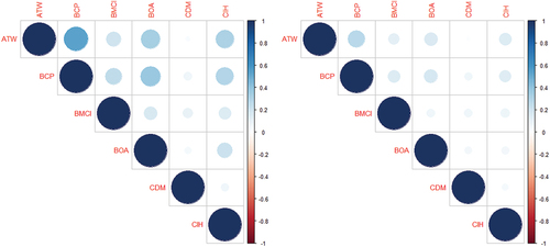
Figure 1 displays the level of bivariate dependence between the log-returns of the six banks’ stocks over the studied period, as measured using Pearson’s correlation and Kendall’s tau. Kendall’s tau is a comprehensive measure of concordance that captures various types of dependencies, while Pearson’s correlation is more appropriate for quantifying linear correlations. Notably, we observe that the stock returns of bank CDM exhibit negligible dependence with all the other banks, indicating a low systemic impact within the considered banking system.

Figure 1. Correlogram: Pearson’s correlation (right) & Kendall’s $\tau$ (Left).

2. Results and discussion

To estimate the upper tail dependence coefficients, we begin by estimating the bivariate copulas between each pair of banks $C(-R_i,-R_j{)}_{i\ne j,i,j\in \{1,\dots ,6\}}$ and between each bank and the banking system $C(-R_i,-R_S{)}_{i=1,\dots ,6}$. The upper tail dependence coefficients between the banks allow us to quantify the impact of a crash in one bank’s value on the other. In the case where the asymptotic dependence is important, we can classify the two banks as being systemic to each other. The bivariate copulas, representing the losses of the banks, are obtained using our entire dataset ($n=1245$ log-returns) with the semi-parametric Canonical Maximum Likelihood (CML) as the method and Akaike Information Criteria (AIC) as the selection criterion. The obtained copulas are presented in Table 5.”S-Gumbel” refers to the Survival Gumbel copula.

Table 5. Estimations of ${\hat{C}}_n-\left(R_i,-R_j\right)$using the CML method with AIC criterion

	BCP	BCI	BOA	CDM	CIH
ATW	t($0.41,3$)	t($0.18,10$)	t($0.24,5$)	Independence	Gumbel ($\theta =1.18$)
BCP		t($0.22,18$)	t($0.27,5$)	Frank ($\theta =0.6$)	t($0.21,5$)
BCI			t($0.12,14$)	S-Gumbel ($\theta =1.07)$	Gumbel ($\theta =1.09$)
BOA				Frank ($\theta =0.53$)	t($0.1,6$)
CDM					S-Gumbel ($\theta =1.04$)

The corresponding bivariate upper tail dependence coefficients are presented in Table 6. We observe the presence of asymptotic dependencies between several pairs of banks. Overall, this dependence remains far from perfect dependence (${\lambda }_U=1$), which indicates the case of comonotonicity of risks, but it remains significant, especially between the banks ATW-BCP, ATW-BOA, and ATW-BCP. This measure of asymmetric dependence is independent of the nature of the marginal behavior as well as the weight of the bank in the system, thus providing an objective quantification of the capacity of a severe loss in one bank’s assets to cause a significant loss in the other.

Table 6. Bivariate upper tail dependence coefficients between banks ${\hat{\lambda }}_{U,n}\left(-R_i,-R_j\right)$

	ATW	BCP	BCI	BOA	CDM	CIH
ATW	1	0.266	0.019	0.104	0.000	0.000
BCP		1	0.003	0.112	0.000	0.094
BCI			1	0.004	0.091	0.000
BOA				1	0.000	0.048
CDM					1	0.049
CIH						1

We adopt a similar approach to compute the coefficients of extreme dependence between each bank and the entire system. Figure 2 presents empirical density plots of copulas between the system and two banks, ATW and CDM. The shapes of these densities reveal the presence of positive dependence between bank ATW and the system, with the dependence being prominent at the tail levels. Conversely, the copula linking bank CDM to the system shows asymptotic independence, indicating a lack of significant dependence.

Figure 2. Density of empirical copula: left (ATW) - right (CDM).

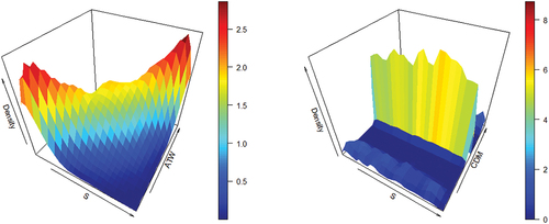
Table 7 displays all the estimated copulas between each bank and the system, while Table 8 presents the corresponding Upper Tail Dependence Coefficients. Figure 3 provides a comprehensive summary of all the relationships of extreme dependence between the banks and the considered banking system.

Figure 3. Extreme interdependence within the Moroccan banking system.

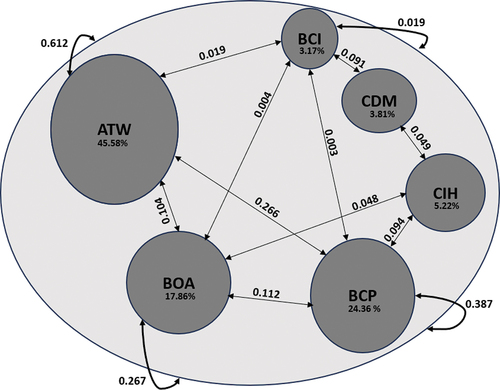
Table 7. Estimations of ${\hat{C}}_n\left(-R_i,S\right)$using the CML method with AIC criterion

	ATW	BCP	BCI	BOA	CDM	CIH
S	t$(0.86,3)$	t$(0.7,4)$	t$(0.33,13)$	t$(0.52,4)$	Gaussian$(0.14)$	Gumbel ($\theta =1.29$)

Table 8. Upper tail dependence coefficients between banks and the System ${\hat{\lambda }}_{U,n}\left(-R_i,S\right)$

	ATW	BCP	BCI	BOA	CDM	CIH
S	0.612	0.387	0.019	0.267	0.000	0.000

Only the two banks, CDM and CIH, are asymptotically independent from the system composed of all the banks. This observation is not directly related to the weight of these banks in the system but rather to the nature of the risk they carry. This is particularly evident in the comparison between the cases of BCI and CIH, for example. However, the strong dependence between the right tails of the losses of the system and those of banks like ATW and BCP is certainly related not only to the nature of the risk but also to their weights in the system, which determine its composition. To confirm these observations, we will also estimate the Upper Tail Dependence Coefficients between each bank and the system composed of the other banks, denoted as ${\lambda }_U(X_i,S_{-i}).$ The estimated copulas and the corresponding upper tail dependence coefficients are presented in Tables 9 and 10, respectively.

Table 9. Estimations of ${\hat{C}}_n\left(-R_i,S_{-i}\right)$using the CML method with AIC criterion

	ATW	BCP	BCI	BOA	CDM	CIH
${\mathbf{S}}_{-\mathbf{i}}$	t$(0.4,3)$	t$(0.45,3)$	t$(0.23,10)$	t$(0.28,4)$	Gaussian$(0.08)$	t$(0.25,5)$

Table 10. Upper tail dependence coefficients ${\hat{\lambda }}_{U,n}\left(-R_i,S_{-i}\right)$

	ATW	BCP	BCI	BOA	CDM	CIH
${\mathbf{S}}_{-\mathbf{i}}$	0.262	0.286	0.024	0.156	0.000	0.107

The coefficients obtained in Table 10 indicate, firstly, that the weight of a bank in the system, as measured by its capitalization, can introduce bias in the quantification of the systemic risk it presents. This effect can occur in both directions; for instance, in the case of the ATW bank, the risk was overestimated due to its significant weight, whereas in the case of the CIH bank, this risk was underestimated. With this last estimation method, BCP has emerged as the bank that exhibits the strongest asymptotic dependence with the rest of the system. Both methods confirm that the banks that can potentially cause the most losses to the system in the event of a decline in their values are ATW, BCP, and BOA.

To deepen our analysis, we now shift our focus to the systemic risk indicators derived from the risk measures TVaR and Expectile. These measures are based on the idea of comparing the weight that a bank $X_i,i=1,\dots ,6$ represents in the system’s risk, without considering dependence, or rather considering perfect dependence that neglects the diversification gain within the system, with the actual weight derived from the Euler risk allocation method, which takes into account the dependence structure between the system’s components. It should be noted that the difference between the two risk measures used lies in the consideration of the bank’s performance through the expectile, while TVaR exclusively measures the risk of losses. The bank’s weight is directly taken into account in the construction of the method since $X_i=-{\alpha }_i{R}_i,i=1,\dots ,6$.

In the first step, we set the threshold to 95% and used the entire database of logarithmic returns. Table 11 presents the values obtained using the two risk indicators. These indicators indicate that a bank exhibits systemic risk when they are negative. In the case of positive values, they suggest that the dependence between the bank and the other components of the system does not generate additional risk. As the indicator’s value increases (moving towards positive values), the risk is perceived to decrease. We can set a tolerance threshold of, for example, 5%, in line with the $\alpha$ threshold.

Table 11. $SR{I}_{TVa{R}_{95\mathrm{\%}}}\left({\alpha }_i{X}_i|S\right)$ and $SR{I}_{e_{95\mathrm{\%}}}\left({\alpha }_i{X}_i|S\right)$

	ATW	BCP	BCI	BOA	CDM	CIH
$SR{I}_{TVa{R}_{95\mathrm{\%}}}\left({\alpha }_i{X}_i|S\right)$	-10.44%	-0.66%	+3.01%	+3.38 %	+2.91%	+1.80%
$SR{I}_{e_{95\mathrm{\%}}}\left({\alpha }_i{X}_i|S\right)$	-10.62%	-1.60%	+3.11%	+4.49 %	+3.03%	+1.60%

According to the results, Bank ATW is identified as systemic by both indicators, and BCP is also systemic without exceeding the 5% threshold. The other banks are not systemic according to these results, and bank BOA represents the least risky component of the system. These findings also suggest that the bank’s weight can contribute to increasing the risk it carries when it is systemic.

To confirm these conclusions, we vary the threshold $\alpha$ between 90% and 99.99%. Figure 4 displays the results obtained for the two systemic risk indicators.

Figure 4. $SR{I}_{TVa{R}_{\alpha }}\left({\alpha }_i{X}_i|S\right)$(Left) and $SR{I}_{e_{\alpha }}\left({\alpha }_i{X}_i|S\right)$ (right) for $\alpha \in \left[0.90,1\right]$.

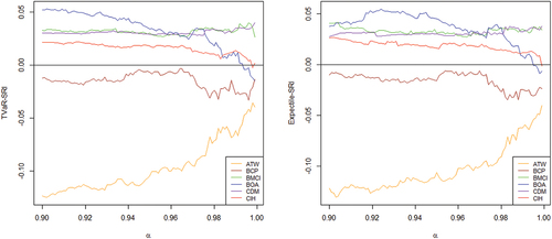
The behavior of the indicators varies depending on the chosen threshold $\alpha$. The instability observed in the resulting curves can be attributed to the presence of nesting estimation errors inherent in the indicator calculations. To address this challenge and enhance the interpretability of our findings, we apply spline smoothing with a fixed parameter value of approximately 1 for all indicators. While this parameter selection lacks specific mathematical criteria, it is intended to emphasize prominent trends within our indicators. Spline smoothing, as a data-driven technique, aids in uncovering underlying patterns in our data. The smoothed curves are presented in Figure 5.

Figure 5. Smoothed spline of $SR{I}_{TVa{R}_{\alpha }}\left({\alpha }_i{X}_i|S\right)$ (Left) and $SR{I}_{e_{\alpha }}\left({\alpha }_i{X}_i|S\right)$ (right).

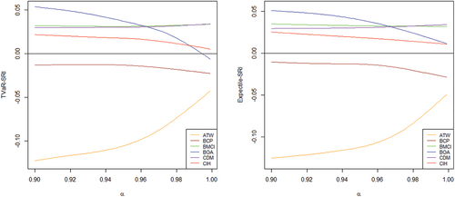
The banks identified as non-systemic, namely BCI and CDM, maintain this status for all values of the threshold $\alpha$, indicating low asymptotic dependence with the rest of the system. Conversely, the banks showing significant extreme dependence, such as BOA and CIH, exhibit positive systemic risk indicators that increase as $\alpha$ approaches 1, indicating higher degrees of risk and approaching the negative zone. This behavior is more pronounced for the indicator based on TVaR, as it solely considers contributions to the system’s losses. With this indicator, BOA becomes systemic at the asymptotic level.

The two systemic banks, ATW and BCP, maintain their systemic status for all threshold values of $\alpha$, with a decrease in risk for ATW. This decrease could be influenced by the increase in systemic risk of other banks at the asymptotic level of $\alpha$, as risk measures severely evaluate all potential loss risks. However, comprehending the asymptotic behavior of the indicators, as $\alpha$ approaches 1, requires specific treatment using extreme value statistics.

In all the previous analyses, we assessed systemic risk using indicators estimated on a 5-year database of stock market quotes. However, this approach does not provide insights into the indicators’ behavior over time. To address this limitation, we employ a dynamic estimation approach. We consider a reference period of one financial year with 252 trading days (1Y). The indicators are calculated using a sliding window, and at each date, $t$, the indicator is estimated using data from the past 252 days (i.e., between dates $t-251$ and $t$). This approach enables us to observe the evolution of the two indicators over a span of four financial years.

The results obtained from this dynamic estimation process for $\alpha =95\mathrm{\%}$ are presented in Figure 6. This approach allows us to gain a better understanding of how our systemic risk indicators fluctuate over time and respond to changing market conditions and economic events.

Figure 6. $1Y-SR{I}_{TVa{R}_{95\mathrm{\%}}}\left({\alpha }_{i,t}{X}_{i,t}|S_t\right)$ (Left) and $1Y-SR{I}_{e_{95\mathrm{\%}}}\left({\alpha }_{i,t}{X}_{i,t}|S_t\right)$ (right).

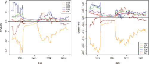
With only slight differences in values between the two indicators, resulting from the distinction between TVaR and Expectile as risk measures, the overall behavior follows similar trends for both indicators. However, we observe significant variations in the corresponding systemic risk indicators, particularly for the two banks ATW and BCP. The other banks remain relatively non-systemic during the 4-years period. To better understand the reasons for these changes for ATW and BCP, which were previously identified as the most systemic within the Moroccan banking system, we compare the evolution of the indicators in their cases with their rolling annual returns:

$R_{i,t}\mathrm{\_}1Y=\prod _{\mathrm{\ell }=0}^{251}\left(1+R_{i,t-\mathrm{\ell }}\right)-1,i=1,\dots ,d.$

Figure 7 presents the curves obtained for the two banks.

Figure 7. ATW (Left)—BCP (right): 1Y $\begin{array}{rl}& R_{i,t}vsSR{I}_{TVa{R}_{95\mathrm{\%}}}\left({\alpha }_{i,t}\hspace{0.17em}{X}_{i,t}|S_t\right)vsSR{I}_{e_{95\mathrm{\%}}}\\ & \left({\alpha }_{i,t}{X}_{i,t}|S_t\right)\end{array}$.

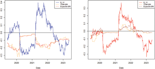
The most notable behavior is observed in the indicators for the BCP bank, which tends to exhibit a higher level of systemic risk during periods of negative performance. In such periods, its systemic risk indicators also become positive, and their evolution closely follows the performance of its returns. On the other hand, the ATW bank remains consistently within the systemic zone throughout the entire 4-year period. Its systemic level decreases (the value of the indicator increases) during periods of losses and increases during periods of gains. This finding suggests that the systemic nature of ATW bank is likely influenced by its weight within the system. During periods of positive returns, its weight in the system increases, leading to a higher systemic risk level. Conversely, during periods of negative returns, the risk decreases due to its reduced weight in the system caused by a decrease in its capitalization.

To sum up, this study identifies two banks, ATW and BCP, as systemic within the Moroccan banking system, consisting of listed banks. The analysis reveals that ATW significantly contributes to the systemic risk, primarily due to its substantial weight within the system, surpassing that of all other components. Similarly, BCP exhibits considerable systemic risk and demonstrates significant extreme dependence with the rest of the system. Consequently, based on these findings, it can be inferred that BCP carries a higher level of systemic risk compared to ATW. The different banks are thus ranked in ascending order of their systemic levels, from the most systemic to the least systemic, as follows: BCP, ATW, BOA, CIH, BCI, and CDM. Notably, the last two banks, BCI and CDM, do not demonstrate an empirical level of risk that qualifies them as systemic within the analyzed context.

Our study has important implications for financial regulators and policymakers in Morocco. It underscores the need for a proactive approach to managing systemic risk in the banking system, particularly among listed banks. Regulators should consider implementing measures such as increasing capital requirements, enhancing liquidity requirements, and strengthening deposit guarantee funds to mitigate systemic risks.

However, it is important to acknowledge the limitations of our study. Our indicators are based on stock market data, which may not fully capture the complexity of systemic risk. Risk can be endogenous and may not always manifest in stock prices. Therefore, our indicators should be used in conjunction with other risk assessment tools for a more comprehensive analysis of systemic risk.

In addition, our study focuses on listed banks and does not account for the entire Moroccan banking system. Future research could expand the scope to include non-listed banks and explore the interconnectedness between different segments of the banking sector.

Overall, our research provides valuable insights into the quantification of systemic risk, but it should be considered alongside its limitations when formulating regulatory strategies.

3. Conclusion

In conclusion, this article introduces simple indicators for identifying systemic banks and quantifying systemic risk. While these indicators provide valuable insights, they do not fully capture endogenous risk not reflected in stock market values.

Our findings underscore the importance for financial regulators, especially in the Moroccan context, to consider individual banks’ risk profiles when implementing risk mitigation measures. This may include raising capital requirements, increasing high-quality liquid assets, and enhancing participation in deposit guarantee funds. Special attention should be given to systemic banks with foreign capital and international branches to address cross-border risks comprehensively.

In summary, our proposed indicators offer valuable insights for identifying systemic risks and guiding regulatory efforts to maintain a stable financial system. However, comprehensive assessments considering endogenous risk and other factors are essential for robust risk management practices.

Disclosure statement

No potential conflict of interest was reported by the author(s).

References

- Acharya, V., Engle, R., & Richardson, M. (2012). Capital shortfall: A new approach to ranking and regulating systemic risks. The American Economic Review, 102(3), 59–19. https://doi.org/10.1257/aer.102.3.59
- Acharya, V., Pedersen, L., Philippon, T., & Richardson, M. (2010). Measuring systemic risk. The Review of Financial Studies, 30(1), 2–47.
- Acharya, V. V., Pedersen, L. H., Philippon, T., & Richardson, M. (2017). Measuring systemic risk. The Review of Financial Studies, 30(1), 2–47. https://doi.org/10.1093/rfs/hhw088
- Adrian, T. and Brunnermeier, M. K. (2011). Covar. Technical report, National Bureau of Economic Research.
- Adrian, T., & Brunnermeier, M. K. (2016). Covar. The American Economic Review, 106(7), 1705. https://doi.org/10.1257/aer.20120555
- Artzner, P., Delbaen, F., Eber, J.-M., & Heath, D. (1999). Coherent measures of risk. Mathematical Finance, 9(3), 203–228. https://doi.org/10.1111/1467-9965.00068
- Bellini, F., & Bignozzi, V. (2015). On elicitable risk measures. Quantitative Finance, 15(5), 725–733. https://doi.org/10.1080/14697688.2014.946955
- Bellini, F., & DiBernardino, E. (2017). Risk management with expectiles. European Journal of Finance, 23(6), 487–506. https://doi.org/10.1080/1351847X.2015.1052150
- Brownlees, C. T., & Engle, R. (2012). Volatility, correlation and tails for systemic risk measurement. Available at SSRN, 1611229. https://doi.org/10.2139/ssrn.1611229
- Castro, C., & Ferrari, S. (2014). Measuring and testing for the systemically important financial institutions. Journal of Empirical Finance, 25, 1–14. https://doi.org/10.1016/j.jempfin.2013.10.009
- El Qalli, Y. and Said, K. (2023). Some systemic risk indicators. https://hal.science/hal-04162836.
- Emmer, E., Kratz, M., & Tasche, D. (2015, December). What is the best risk measure in practice? A comparison of standard measures. Journal of Risk, 18(2), 31–60. https://doi.org/10.21314/JOR.2015.318
- Firano, Z. (2015). Systemic risk and financial contagion in morocco: New approaches of quantification. In Overlaps of Private sector with public sector around the globe (Vol. 31, pp. 141–171). Emerald Group Publishing Limited.
- Frahm, G., Junker, M., & Schmidt, R. (2005). Estimating the tail-dependence coefficient: Properties and pitfalls. Insurance: Mathematics and Economics, 37(1), 80–100. https://doi.org/10.1016/j.insmatheco.2005.05.008
- Ghosh, B., & Krishna, M. C. (2019). Power law in tails of bourse volatility–evidence from india. Investment Management & Financial Innovations, 16(1), 291–298. https://doi.org/10.21511/imfi.16(1).2019.23
- Ghosh, B., Le Roux, C., & Verma, A. (2020). Investigation of the fractal footprint in selected euribor panel banks. Banks and Bank Systems, 15(1), 185. https://doi.org/10.21511/bbs.15(1).2020.17
- Gnedenko, B. (1943). Sur la distribution limite du terme maximum d’une serie aleatoire. Annals of Mathematics, 44(3), 423–453. https://doi.org/10.2307/1968974
- Hill, B. M. (1975). A simple general approach to inference about the tail of a distribution. The Annals of Statistics, 3(5), 1163–1174. https://doi.org/10.1214/aos/1176343247
- Jenkinson, A. F. (1955). The frequency distribution of the annual maximum (or minimum) values of meteorological elements. Quarterly Journal of the Royal Meteorological Society, 81(348), 158–171. https://doi.org/10.1002/qj.49708134804
- Joe, H. (1997). Multivariate models and multivariate dependence concepts. CRC Press.
- Knaup, M., & Wagner, W. (2012). Forward-looking tail risk exposures at U.S. Bank Holding Companies. Journal of Financial Services Research, 42(1–2), 35–54. https://doi.org/10.1007/s10693-012-0131-5
- Kyoud, A., El Msiyah, C., & Madkour, J. (2023). Modelling systemic risk in morocco’s banking system. International Journal of Financial Studies, 11(2), 70. https://doi.org/10.3390/ijfs11020070
- Löffler, G. and Raupach, P. (2013). Robustness and informativeness of systemic risk measures. Deutsche Bundesbank.
- Mainik, G., & Schaanning, E. (2014). On dependence consistency of covar and some other systemic risk measures. Statistics & Risk Modeling, 31(1), 49–77. https://doi.org/10.1515/strm-2013-1164
- Maume-Deschamps, V., Rullière, D., & Said, K. (2017). Multivariate extensions of expectiles risk measures. Dependence Modeling, 5(1), 20–44. https://doi.org/10.1515/demo-2017-0002
- Maume-Deschamps, V., Rullière, D., & Said, K. (2018). Extremes for multivariate expectiles. Statistics & Risk Modeling, 35(3–4), 111–140. https://doi.org/10.1515/strm-2017-0014
- NECHBA, Z. B. (2021). Moroccan conventional banks’ contribution to systemic risk. International Journal of Business and Technology Studies and Research, 3(3), 10.
- Newey, W. K., & Powell, J. L. (1987, July). Asymmetric least squares estimation and testing. Econometrica, 55(4), 819–847. https://doi.org/10.2307/1911031
- Oakes, D. (1994). Multivariate survival distributions. Journal of Nonparametric Statistics, 3(3–4), 343–354. https://doi.org/10.1080/10485259408832593
- Said, K. (2023). Expectile-based capital allocation. International Journal of Analysis and Applications, 21, 79. https://doi.org/10.28924/2291-8639-21-2023-79
- Sklar, M. (1959). Fonctions de répartition à n dimensions et leurs marges. Annales de l’ISUP, 8(3), 229–231.
- Wang, S. S. (2000). A class of distortion operators for pricing financial and insurance risks. The Journal of Risk and Insurance, 67(1), 15–36. https://doi.org/10.2307/253675