Modeling the characteristics and quantification of adulterants in gasoline using FTIR spectroscopy and chemometric calibrations

Abstract

The criminal act of fuel (gasoline) adulteration still remains a global worry due to its environmental, health and economic effect. Current methods for the detection of fuel adulteration have not been effective in most developing countries due to the associated cost of implementation. Therefore, there is the need for a fast, reliable and cheaper approach for screening of adulterants in fuel. This study combined FTIR analyses with Chemometric (multivariate) techniques for qualitative and quantitative determination of four possible adulterants: kerosene, diesel, naphtha and premix in gasoline. Synthetic admixtures prepared by mixing the gasoline with varying proportions of the adulterants were obtained and used for the model calibration. Soft Independent Modeling Class Analogy (SIMCA) classification and Partial Least Square (PLS) regression methods were the Chemometric techniques employed. The SIMCA classification model developed predicted the type of adulterant present at an error rate of 6.25% for Kerosene and naphtha, and 12.5% for premix. However, no prediction error was recorded for classifying samples contaminated with diesel. The PLS regression model was able to predict the concentrations of adulterant with prediction errors lower than 5% for all adulterants considered. Applying the models to commercial gasoline samples collected from a Metropolis in Ghana revealed 7% gasoline adulteration with kerosene (4%), premix (2%) or diesel (1%). No adulteration with naphtha was detected. The FTIR-Chemometric approach proved a fast and cheaper method for detection of adulteration which can be adopted by quality assurance and monitoring laboratories for forensic screening of gasoline in Ghana

Keywords:

• adulteration
• fuels
• characterization
• quantification
• spectroscopy
• chemometrics

PUBLIC INTEREST STATEMENT

Fuels, such as gasoline, are basically used in our vehicles. However, there are other types of fuels, such as kerosene and diesel, which are also used for other purposes. Fuels can be adulterated, that is by mixing two or more fuel types to form a mixture. This adulterated fuel has serious consequences such as pollution of the environment when burnt in the open, as well as its effect on the engines. Governments in developing countries are cracking down perpetrators of fuel adulteration. This work looks at developing a fast and vigorous method that is cheap and easy to detect and quantify adulterated fuels. From the research work, we have been successful in developing a technique to achieve our aim. This technique can be used by governments’ agencies, such as environmental protection agencies, filling station operators and any other activity that employs the use of liquid fuels. This method will give liquid fuels users an idea about the purity of their product.

1. Introduction

The incidence of fuel adulteration continues to exist globally, especially in developing countries. The situation has gained public attention due to its devastating economic and environmental effects. The intentional blending of high-grade gasoline and diesel with lower grade ones, other cheaper products and solvents in an attempt to maximize profit has shown to have stiffening effects on a national economy and this is a major concern for most countries. Adulterated fuels often result in low engine performance and engine life. It has also been proven that combustible engines with adulterated fuels often produce excessively high quantities of tailpipe emissions of harmful products, hence its environmental concerns (Ale, 2003). The differences in the prices of different petroleum products have been the major driving force for adulteration. In attempt to minimize these losses, several regulatory schemes are being adopted by most countries, especially to detect adulterated fuel, punish culprits and deter potential fraudsters. Over the years, several analytical techniques have been employed in the detection of fuel adulteration, from the use of physicochemical parameters to the use of spectroscopic (Patra, Sireesha, & Mishra, 2000) and chromatographic fingerprinting methods (Pedroso, De Godoy, Ferreira, Poppi, & Augusto, 2008). Recently, fuel marking has proven the best detection technique. This technique has also been used since 2014 in Ghana under the Petroleum Product Marking Scheme. Despite the efficiency of this technology, both marking and/or detection are extremely expensive and as such, countries have to spend millions of dollars on each batch of petroleum product. Due to the confidentiality and exclusivity of this technique, few laboratories are equipped and mandated to perform these analyses which are often burdened with the task of analyzing massive numbers of samples. The time-consuming and laborious nature of the analytical technique also propels most laboratories to randomly select and analyze only few of the samples presented at any time. In Brazil, only 10% of commercial gasoline samples selected are subjected to solvent tracer analysis (Tanaka, De Oliveira Ferreira, Ferreira Da Silva, Flumignan, & De Oliveira, 2011). There is therefore the need to develop rapid, less expensive techniques that can be used to screen and predict adulteration of commercial fuel. Current developments have proved the feasibility of Chemometric techniques such as Hierarchical Cluster Analysis, Principal Component Analysis (PCA), Least Discriminant Analysis, Soft Independent Modeling of Class Analogy (SIMCA) and Successive Progression Algorithm as an important tool applied to the fast detection of fuel adulteration. However, no such study has been conducted in Ghana. This study therefore seeks to apply such Chemometric tools to develop models that can be used to preliminary screen and predict adulteration of gasoline on the Ghanaian Market.

2. Materials and methods

• Experimental approach was employed in building the predictive models (SIMCA and PLS): phase I. Only primary data obtained in the experiment was used. For phase II, a cross-sectional survey approach was adopted to assess the level of adulteration in commercial gasoline samples in Ghana using the constructed model.

• Commercial gasoline samples for the external validation of the model (phase II) were purchased from various fuel outlets in the Kumasi Metropolis in the Ashanti region of Ghana. Fuel outlets were selected from all sub-metro in Kumasi.

2.1. Sample collection

All pure and quality samples (gasoline, diesel, kerosene, premix fuel and light naphtha) for the experimental phase were supplied by the Inspectorate Ghana Limited. The gasoline samples were kept in dark bottles in a refrigerator before use. For the external validation of the model, 100 commercial gasoline samples were purchased from different filling stations in the Kumasi Metropolis using cluster sampling technique. All samples were kept in Polyethylene Terephthalate bottles and stored in a cool dry place prior to analysis.

2.2. Experimental phase

2.2.1. Sample preparation

Synthetic mixtures were prepared by mixing the gasoline (base fuel) with varying amounts of each selected adulterants (kerosene, premix, naphtha) to cover the range of 5–50% v/v as shown in Table 1.

Table 1. Ratio of gasoline–adulterant admixture prepared in the laboratory

Sample no.	% v of gasoline–kerosene mixture (GK)	% v of gasoline–premix mixture (GP)	% v of gasoline–naptha mixture (GN)	% v of gasoline–diesel mixture (GD)
1	95:5	95:5	95:5	95:5
2	90:10	90:10	90:10	90:10
3	85:15	85:15	85:15	85:15
4	80:20	80:20	80:20	80:20
5	75:25	75:25	75:25	75:25
6	70:30	70:30	70:30	70:30
7	65:35	65:35	65:35	65:35
8	60:40	60:40	60:40	60:40
9	50:50	50:50	50:50	50:50

2.2.2. Instrumental analysis

Instrumental analysis was performed at the Central Laboratory of the Kwame Nkrumah University of Science and Technology, Kumasi, Ghana. The neat fuel (control) and synthetic mixtures were analyzed using a PerkinElmer FTIR spectrometer to obtain their distinctive spectral fingerprints.

Each spectrum was obtained within the range of 400–500 cm⁻¹ wavenumber with a resolution of 4 cm⁻¹ and scanned 64 times. Each mixture was run in triplicate and the sample area cleaned twice with acetone in between runs. The mean spectra as well as absorbance data and their corresponding wavenumber for each sample were recorded.

2.2.3. Chemometric analysis

The spectral data obtained were then used in the calibration and validation of the predictive models. Chemometric analysis was done using the PLS Toolbox 8.1 with MATLAB R2012a. The samples for each class of adulterant were divided into two sets: calibration (training set) and the validation (test set).

A classification (SIMCA) model was built using the data obtained from the FTIR analysis of the calibration set. Several processing techniques involving Mean Centralization, derivation and Multiplicative Scatter Correction were applied to all or portions of the spectra to obtain a more accurate PCA sub-models for each class (adulterant). The four PCA models were then assembled as the SIMCA model. A PLS regression model was also built for each class of adulterant based on the absorbance and concentrations of adulterants added to the base fuel. All models were validated by internal cross-validation and also by using a different set of data (external validation set).

The predictive capacity of each of the models were determined using calculated parameters such as optimum number of latent variables, Root Mean Square Error of validation, Root Mean Square Error of calibration, coefficient correlation of calibration and coefficient correlation of validation. The models with the best predictive capacity were selected and validated.

2.3. Cross-sectional phase

The commercial samples purchased were also subjected to FTIR spectral analysis using the PerkinElmer FTIR spectrometer under the same conditions as used for the calibration set. The built classification model (SIMCA) was applied to the obtained data to predict the type of adulterant (if any) present. The concentration of the adulterant present in the samples classified as adulterated was then determined using the appropriate PLS model.

3. Results and discussions

3.1. FTIR analysis of standard petroleum products

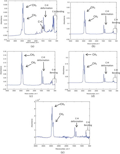
The standard (neat) fuel samples, gasoline (base fuel), diesel, kerosene, naphtha and premix (possible adulterants) were supplied by the Inspectorate Ghana Limited. The standard samples were analyzed using the FTIR spectrometer. The respective spectra obtained for each sample are shown in Figure 1. Most samples absorbed at the same wavenumber with slight differences in the degree of absorbance.

Figure 1. Spectrum of pure gasoline (a), diesel (b), kerosene (c), premix (d), naphtha (e).

3.2. FTIR analysis of fuel admixture

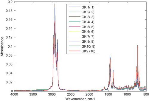
3.2.1. Gasoline–kerosene mixture

To calibrate the models, adulteration of fuels were simulated in the laboratory. Ten synthetic mixtures prepared by adding different concentrations of kerosene (5–50% v/v) to the base fuel (gasoline) were each subjected to FTIR analysis and their resulting respective spectrum are superimposed in Figure 2. The spectra showed strong overlaps almost at the entire spectral range. At wavenumbers with significantly high absorption, absorption barely correlated with the concentration of adulterant (kerosene) added.

Figure 2. Spectra of gasoline–kerosene mixtures at different concentrations.

Samples GK1-GK10 are gasoline–kerosene admixtures with concentrations of kerosene from 5–50% v/v, respectively.

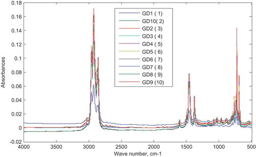
3.3. FTIR analysis of gasoline–diesel admixtures

Admixtures prepared by addition of different concentrations of diesel to the gasoline were also analyzed using the FTIR spectrometer. Figure 3 shows the superimposed spectrum of each prepared mixture.

Figure 3. Spectra of gasoline-diesel mixtures at different concentrations.

Samples GD1-GD10 are gasoline–diesel admixtures with concentrations of diesel from 5–50% v/v, respectively.

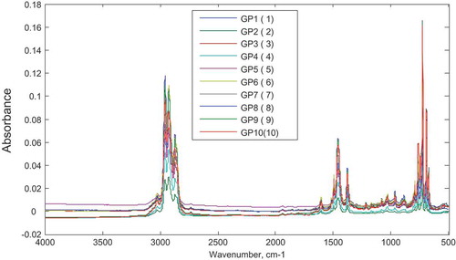
3.4. FTIR analysis of gasoline–premix admixtures

Ten mixtures of gasoline–premix were also prepared in the laboratory at varying concentrations (5–50% v/v). Each individual mixture was subjected to FTIR analysis and the obtained spectra are superimposed in Figure 4. Strong overlapping regions were observed among the individual spectrum across the spectra range.

Figure 4. Spectra of gasoline–premix mixtures at different concentrations.

Samples GP1-GP10 are gasoline–diesel admixtures with concentrations of premix from 5–50% v/v, respectively

3.5. FTIR analysis of gasoline–(L) naphtha admixtures

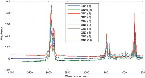
The synthetic mixtures prepared by addition of varying concentrations of the L-naphtha to the gasoline were also analyzed using the FTIR. The absorbance spectrum obtained for each mixture over the range of 4000–500 cm⁻¹ is shown in Figure 5. The spectra showed strong overlap at almost the entire range and absorbance barely correlated with the amount of L-naphtha added.

Figure 5. Spectra of gasoline–naphtha mixtures at different concentrations.

Samples GN1-GN10 are gasoline–diesel admixtures with concentrations of naphtha from 5–50% v/v, respectively.

3.6. Chemometric analysis

3.6.1. Classification by SIMCA

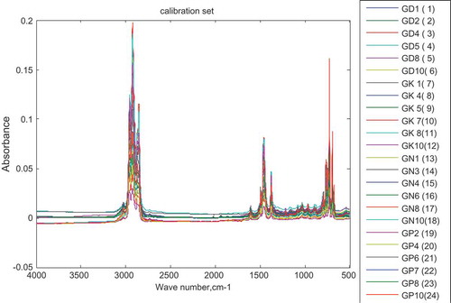
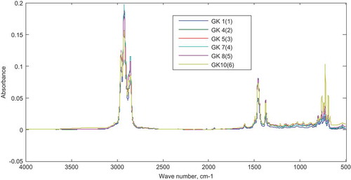
To determine the type of adulterant present in gasoline samples, SIMCA was adopted. SIMCA is able to classify samples as belonging to a predefined class (in this case adulterant) based on established rules (Dago Morales, Cavado Osorio, Fernández, & Dennes, 2008). To develop the SIMCA model, six samples from each class (each class is adulterated with either of the four considered) adulterants were selected for the calibration of the data. Each sample was predefined as belonging to one of the four classes (kerosene, diesel, premix and naphtha) based on the adulterant added. Figure 6 shows the FTIR spectra of the calibration set for the SIMCA model.

Figure 6. Spectra of calibration set for SIMCA model.

Samples with labels GD are adulterated with diesel, GK with kerosene, GP with premix and GN with L-naphtha.

SIMCA was chosen because of its usually good classification results compared to other classification techniques, such as SVM and PCDA as reported by Smit (2009). PCA sub-models were first created for each class set. For each class set, 3PCs accounted for more than 95% of the total variability of the data and hence were selected in building each sub-model.

Preprocessing techniques involving second-order derivative, Multiplicative Scatter Correction (mean) and mean centering of each data were applied to achieve lower errors of calibration at 95% confidence interval. From the detailed information for each PCA sub-model for the various class sets, percent variation captured by PCA model is shown in Tables 2–5 below:

Table 2. Percent variance captured by PCA model–diesel class

Principal component number	Cov (X)	%Variance—this PCA	%Variance—total
1	1.07 × 10^−8	62.63	62.63
2	5.70 × 10^−9	33.30	95.93
3	5.81 × 10^−10	3.40	99.33

All PCA sub-models were built using the Singular Value Decomposition (SVD) algorithm. PCA, by using SVD algorithm, is able to reduce high-dimensional data into fewer dimensions while maintaining the relevant information in the data set. The individual sub-models were then assembled by SIMCA. The confusion matrix of the developed model using the calibration data set is shown in Table 6.

Table 3. Percent variance captured by PCA model–kerosene class

Principal component number	Cov (X)	%Variance—this PCA	%Variance—total
1	1.22 × 10^−5	94.76	94.76
2	4.09 × 10^−7	3.17	97.93
3	2.50 × 10^−7	1.94	99.86

Table 4. Percent variance captured by PCA model–naphtha class

Principal component number	Cov (X)	%Variance—this PCA	%Variance—total
1	2.47 × 10^−9	80.30	80.30
2	5.23 × 10^−10	17.01	97.32
3	5.95 × 10^−11	1.94	99.25

Table 5. Percent variance captured by PCA model–premix class

Principal component number	Cov (X)	%Variance—this PCA	%Variance—total
1	9.36 × 10^−9	74.81	74.81
2	2.14 × 10^−9	17.14	91.95
3	9.24 × 10^−10	7.39	99.33

Table 6. Confusion matrix (A) and confusion table (B) for the calibration set

A
	TPR	FPR	TNR	FNR	N	Err	P	F1
Diesel	1.00	0.00	1.00	0.00	6	0.00	1.00	1.00
Kerosene	1.00	0.00	1.00	0.00	6	0.00	1.00	1.00
Naphtha	1.00	0.00	1.00	0.00	6	0.00	1.00	1.00
Premix	1.00	0.00	1.00	0.00	6	0.00	1.00	1.00
B
	Actual class
	Diesel		Kerosene		Naphtha		Premix
Predicted as diesel	6		0		0		0
Predicted as kerosene	0		6		0		0
Predicted as naphtha	0		0		6		0
Predicted as premix	0		0		0		6

Note: TPR—true positive rates; FPR—false positive rates; TNR—true negative rates; N—number of samples; Err—error rate; P—precision; F1—F scores.

3.6.2. Validation of the SIMCA model

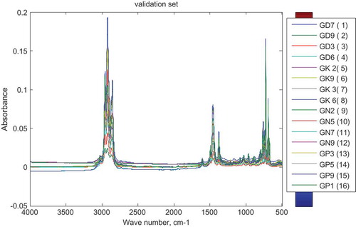
To validate the calibrated model, 16 different samples were prepared in the laboratory by mixing the gasoline with the different adulterants under consideration. Four samples each were mixed with one of the adulterants under consideration. The mixtures were first subjected to FTIR analysis under the same conditions as the calibration set and the resulting spectra are shown in Figure 7.

Figure 7. Spectra of validation (test) set for SIMCA.

Samples with labels GD are adulterated with diesel, GK with kerosene, GP1 with premix and GN with L-naphtha

The classes of the validation data set were predicted using the calibrated model and the result is summarized in Table 7. The model showed excellent precision for all the four modeled sub-classes and also excellent sensitivity and specificity for classifying samples adulterated with diesel.

Table 7. Confusion matrix (A) and confusion table (B) for the validation set

A
	TPR	FPR	TNR	FNR	N	Err	P	F1
Diesel	1.00	0.00	1.00	0.00	4	0.0000	1.00	1.00
Kerosene	0.75	0.00	1.00	0.25	4	0.0625	1.00	0.857
Naphtha	0.75	0.00	1.00	0.25	4	0.0625	1.00	0.857
Premix	0.50	0.00	1.00	0.50	4	0.1250	1.00	0.667
B
	Actual class
	Diesel		Kerosene		Naphtha		Premix
Predicted as diesel	4		0		0		0
Predicted as kerosene	0		3		0		0
Predicted as naphtha	0		0		3		0
Predicted as premix	0		0		0		2

Note: TPR—true positive rates; FPR—false positive rates; TNR—true negative rates; N—number of samples; Err—Error rate; P—precision; F1—F scores.

However, it had an error rate of 6.25% for samples adulterated with kerosene and naphtha as a sample each was not correctly classified (refer to confusion table). Classification of samples adulterated with premix into the said class had an error rate of 12.50%. Despite these error rates, the results revealed that the model had 100% specificity for each modeled class. That is, each modeled class was capable of rejecting any sample that did not belong to it. Further investigations showed that the error rates are attributed to samples that were not assigned to any of the modeled classes other than been wrongly assigned to a class as shown in the Table 8. Samples GN2, GK2, GP9 and GP1 were not assigned to any of the modeled classes.

Table 8. Actual and predicted adulterants present in validation set

Sample ID	Actual class	Predicted class
GD7	1	1
GD9	1	1
GD3	1	1
GD6	1	1
GN2	3	0
GN5	3	3
GN7	3	3
GN9	3	3
Sample ID	Actual class	Predicted class
GK2	2	0
GK9	2	2
GK3	2	2
GK6	2	2
GP3	4	4
GP5	4	4
GP9	4	0
GP1	4	0

Note: 0—unassigned; 1—diesel; 2—kerosene; 3—naphtha; 4—premix.

3.7. PLS model for quantification of kerosene in gasoline (PLS-K)

For each gasoline sample classified as adulterated, it is expedient to determine the quantity of the adulterant present. In this research, a PLS regression approach was adopted. This method was chosen based on its feasibility as a Chemometric technique for the determination of adulterant content present in gasoline as proven by Teixeira, Oliveira, Dos Santos, Cordeiro, and Almeida (2008). In developing a PLS model for the quantitative determination of kerosene in gasoline, 10 synthetic mixtures were prepared by mixing pure gasoline with varying concentrations of kerosene to cover the percentage of 5–50% v/v. Six of the samples were used for the calibration (calibration set) of the model and the other set (test set) for validation.

3.8. Building of PLS model for quantification of kerosene in gasoline

Six gasoline samples adulterated with different concentrations of kerosene ranging from 5–50% v/v (calibration set) were subjected to FTIR analysis and the result is shown in Figure 8.

Figure 8. Spectra of calibration data set for PLS-K.

Several regions of the spectra were tried and the region that appeared well-suited for constructing the mode based on the resulting calibration parameters was chosen.

The spectra region between 650 and 551 cm⁻¹ yielded the best predictive model. The absorbance data obtained for the above region were preprocessed by mean centering the data before used in the calibration. The results were cross-validated using the leave-one-out method as proposed by Haaland and Thomas (1988). The number of optimum factors which yielded the minimum error of calibration and yet maintained the variability in the data was selected.

After applying the cross-validation (leave-one-out), two latent variables were able to explain 99.95% variability in the entire data and corresponded to a minimum root mean square error (RMSE). Hence, two latent variables were found to be optimum for the calibration of the PLS model. The percent variance captured by regression model is summarized in Table 9 below.

Table 9. Percent variance captured by regression model

	X Block		Y Block
Comp	This	Total	This	Total
1	99.30	99.30	74.98	74.98
2	0.63	99.95	20.70	95.69

Sample statistics and scores obtained for the calibration sets were determined. All the samples had statistical values within the limits for Hoteling T² residual, Q residual, leverage and studentized residual. The plot and table of measured vs. predicted concentrations gives a clearer predictive capacity of the model as elaborated in Figure 9.

Figure 9. Measured vs. predicted concentration of kerosene in the calibration set.

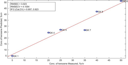
Table 10 indicates the actual and predicted concentration of kerosene in calibration set.

Table 10. Actual and predicted concentration of kerosene in calibration set

Sample ID	Actual:Conc. Kerosene (% v/v)	Predicted:Conc. Kerosene (% v/v)	p-Value (at 0.05 significance level)
GK1	5	5	0.884
GK4	20	25
GK5	25	27
GK7	35	27
GK8	40	42
GK10	50	51

3.9. Validation of the model

The concentrations of kerosene in the validation (test) data sets were predicted using the PLS model developed above. For this set, all analytical procedures including the FTIR scanning and model calibration were repeated under same conditions.

The score plots and sample statistics obtained after applying the model to the validation data set were also determined. The model was applied to same spectra range (650–551 cm⁻¹) as used in the calibration .All samples had Q and T² residuals within limits except sample GK9 which showed high Q residual. However, overall, the model had a good predictive capacity for the validation set as well, as is evident from the actual vs. predicted plot in Figure 10 below.

Figure 10. Actual vs. predicted concentration for the validation set (PLS-K).

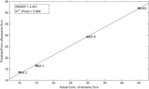
Table 11 indicates the actual and predicted concentration of kerosene in calibration set.

Table 11. Actual and predicted concentration of kerosene in validation set

Sample ID	Actual:Conc. Kerosene (% v/v)	Predicted:Conc. Kerosene (% v/v)	p-Value (at 0.05 significance level)
GK2	10	14	0.622
GK9	45	42
GK3	15	16
GK6	30	29

3.10. PLS model for the quantification of diesel in adulterated gasoline (PLS-D)

To quantify the amount of diesel in diesel-adulterated gasoline samples, another PLS regression model was developed. In building the model, 10 synthetic samples were prepared by mixing pure gasoline with diesel in varying proportions ranging from 5–50% v/v, these were then divided into two sets, six samples for the calibration of the model (calibration set) and four for validation of the model (validation set).

3.11. Building the PLS model

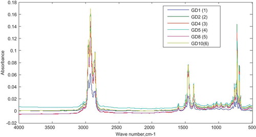
The six samples in the calibration set were subjected to FTIR analysis. Figure 11 shows the FTIR spectra of the samples obtained over the range of 500–400 cm⁻¹ at a resolution of 4 cm⁻¹ and after 64 scans.

Figure 11. Spectra of the calibration data set for PLS-D.

Samples GD1, GD2, GD4, GD5, GD8 and GD10 are adulterated gasoline with 5%, 10%, 20%, 25%, 40% and 50% v/v of diesel, respectively.

The spectra region between the range of 1472–1447 cm⁻¹ appeared more suitable as it gave better model results compared to the others and so was selected for the calibration. The absorbance data obtained at this range was preprocessed before being used in the model building.

Several preprocessing techniques and a combination of these were tried and the one(s) that had the best influence on the predictive capacity of the model was selected. All data were filtered using a second-order Savitzky–Golay derivation approach and normalized using Multiplicative Signal Correction before they were mean centered. The model was first validated using the “leave-one-out” approach as proposed by Haaland and Thomas. To avoid overfitting of the model, the optimum number of latent variables was first selected. The number of latent variables or factors that would yield the least RMSE and still give an appreciable variability in the data set was selected.

In this model, four latent variables chosen were able to account for all the variability in the data with a minimum error of 1.9338 even after cross-validation. Score plots and other sample statistics were obtained after cross-validation of the model. All samples had good statistical values within the limits set for Hoteling T², Q and studentized residuals, as well as leverage.

To assess the predictive capacity of the PLS-D, the measured vs. predicted plot is elaborated in Figure 12.

Figure 12. Actual vs. predicted concentration of diesel in calibration set (PLS-D).

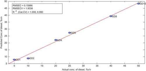
Table 12 show predicted concentrations were further compared with the actual concentrations by means of paired-sample t test and a p-value of 0.390 was obtained at 95% confidence interval.

3.12. Validation of the PLS-D model

The concentrations of diesel in the four samples belonging to the validation set were predicted by the model to serve as an external validation for the model. For the validation data set, all analytical techniques including FTIR scanning conditions, spectra range, data preprocessing, and cross-validation were maintained as for the calibration set. Samples GD3 and GD6 had high Q residuals above the limit at 95% confidence interval. All the samples in the validation set, however, showed low residuals for Hoteling T². To determine the model’s performance, the plot of Y measured vs. Y predicted is elaborated below in Figure 13 with the associated R² and RMSE values.

Figure 13. Actual vs. predicted concentration of diesel in the validation set.

To assess the difference in concentrations of the predicted and actual values, a paired-sample t test was performed at 95% confidence interval and the result are shown in Tables 12 and 13.

Table 12. Comparison of actual and predicted diesel concentration in calibration set

Sample ID	Actual concentration of diesel (% v/v)	Predicted concentration of diesel (% v/v)	p-Value (at 0.05 significance level)
GD1	5	8	0.390
GD2	10	9
GD4	20	22
GD5	25	27
GD8	40	39
GD10	50	48

Table 13. Comparison of actual and predicted diesel concentration in validation set

Sample ID	Actual:Conc. Diesel (% v/v)	Predicted:Conc. Diesel (% v/v)	p-Value (at 0.05 significance level)
GD9	45	44	0.812
GD3	15	17
GD6	30	34
GD7	35	38

A p-value >0.05 was obtained.

3.13. PLS model for the quantification of naphtha in adulterated gasoline (PLS-N)

3.13.1. Constructing the PLS model (PLS-N)

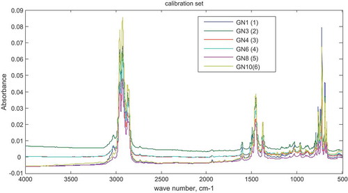
Six synthetic admixtures with naphtha concentration ranging from 5% to 50% v/v in the calibration set were first analyzed using FTIR and the spectra results obtained over the range of 4000–500 cm⁻¹ at a resolution of 4 cm after 64 scans are superimposed in Figure 14.

Figure 14. Spectra of (L) naphtha-adulterated gasoline samples (calibration set).

The 3501 data points for the absorbance over the entire spectral range were preprocessed and used for the calibration of the model. The preprocessing involved a second-order Savitzky–Golay derivation, Multiplicative Signal Correction and then mean centering. Cross-validation of the model was done using the Haaland and Thomas approach of “leave-one-out”.

To construct the model, the optimum number of latent variables (factors) necessary was selected. Four latent variables were able to explain 99.80% variability in the data and still give a model with RMSE of 0.998 after cross-validation as shown below. Hence, four latent variables were selected for constructing the model. The sample statistics obtained after the cross-validation of the model together with other score plots were determined.

The Y measured vs. Y predicted plot is elaborated below with its associated R² and RMSE values to easy assessment of the predictive capacity of the model as shown in Figure 15.

The actual and predicted concentrations of diesel in the samples were compared further using paired-sample t test and p-value of 0.993 was obtained as shown in Table 14.

Table 14. Comparison of actual and predicted naphtha concentration in calibration set

Sample ID	Actual:Conc. Naphtha in gasoline (% v/v)	Predicted:Conc. Naphtha in gasoline (% v/v)	p-Value (at 0.05 significance level)
GN1	5	6	0.993
GN3	15	13
GN4	20	21
GN6	30	30
GN8	40	39
GN10	50	50

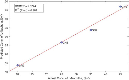
3.13.2. Validating the PLS model

As a means of also validating the model, four of the synthetic mixtures (validation or set) with concentrations of naphtha different from those of the calibration set were selected. These samples were also first subjected to FTIR analysis. For the FTIR analysis, all parameters/calibration including spectral range, resolutions and scanning were maintained as for the calibration set. The calibrated model was then applied to the absorbance data to predict the concentration of naphtha in the samples.

All analytical techniques and model parameters such as spectra range, preprocessing and cross-validation were set at equal conditions as that of the calibration set. The performance of the model on the validation set was determined. Sample GN2 had extremely high Q residual; however, all samples had low Hoteling T² residual below the statistical limit. Elaboration and further comparison of the measured and predicted concentrations of L-naphtha are presented in Figure 16 and Table 15, respectively. No statistical difference was observed between actual and predicted concentration of naphtha in the samples (p > 0.05).

Table 15. Comparison of actual and predicted naphtha concentration in validation set

Sample ID	Actual:Conc. L-naphtha Sample (% v/v)	Predicted:Conc. L-naphtha Sample (% v/v)	p-Value (at 0.05 significance level)
GN2	10	14	0.886
GN5	25	27
GN7	35	34
GN9	45	47

Figure 15. Actual vs. predicted concentrations of naphtha in the calibration set.

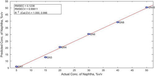
Figure 16. Actual vs. predicted concentration of naphtha (validation set).

3.14. PLS model for the quantification of premix in adulterated gasoline (PLS-P)

A PLS regression model for the quantification of premix as an adulterant in gasoline was also constructed. As in the previous models, 10 synthetic gasoline–premix mixtures were used for calibration (6 samples) and validation (4 samples) of the model. The mixtures were prepared to cover the range of 5–50% v/v of the premix in the gasoline.

3.14.1. Constructing the PLS model

Six out of the ten synthetic mixtures were chosen for the calibration of the model. Each sample was first subjected to FTIR analysis and the results are shown in Figure 17. The FTIR spectra were obtained over the range of 4000–500 cm⁻¹ after 64 scans with a 4-cm resolution.

The spectral region 1503–1361 cm⁻¹ was chosen for the calibration of the model. This region yielded a model with higher prediction capacity compared to others and the entire spectra as well. Before the calibration, all the absorbance data within this range were first normalized and then a second-order Savitzky–Goaly derivation was then applied. A cross-validation technique (leave-one-out) was then set to internal validate the model after calibration. The number of latent variables that explained most of the variability and yet kept a minimum error of calibration was chosen for the construction of the model.

Four latent variables were selected for the calibration of the model due to its associated minimum error of calibration. The four latent variables also explained 100% variance in the data. Percent variation capture by regression model is shown in Table 16.

Table 16. Percent variance captured by regression model

	X Block		Y Block
Comp		Total		Total
1	62.25	62.25	90.55	90.55
2	20.38	85.63	90.09	99.62
3	10.70	96.32	0.22	99.85
4	3.23	99.55	0.14	99.99

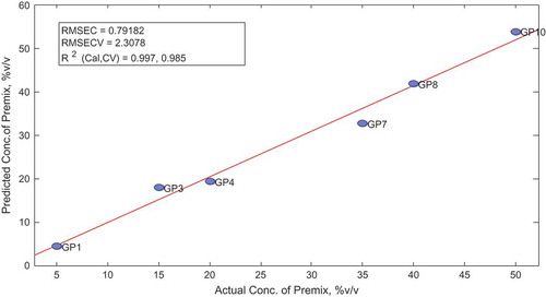
The sample statistics and score obtained after the calibration and cross-validation of the model are summarized. The plot of actual vs. predicted concentrations is illustrated below showing the model performance parameters, such as the errors of calibration and coefficient of calibration. Comparison using paired-sample t test revealed no statistical difference between actual and predicted concentration of premix in the adulterated gasoline is shown in Figure 18.

Figure 17. Spectra of gasoline samples adulterated with premix (calibration set).

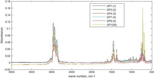
Figure 18. Actual vs. predicted concentration of premix (calibration set).

3.14.2. Validating the PLS-P model

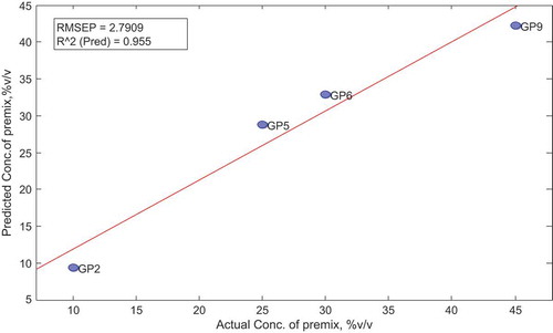
To test the performance of the calibrated model, it was further applied to a different set of data (validation set) to determine if the model can predict correctly the actual concentrations in that set as well. The validation samples were also subjected to FTIR analysis under the same conditions as the calibration set (see Table 17). The model was applied to the absorbance data within the same range (1503–1361 cm⁻¹) as for the calibration. All other analytical techniques including the data preprocessing and cross-validation were set at same conditions as that of the calibration set. The sample statistics and scores were obtained after applying the model. The elaborated actual vs. predicted plot in Figure 19 showed that the model had less than 3% (RMSEP of 2.791) prediction errors in prediction concentration of premix in the adulterated gasoline samples in the validation set.

Figure 19. Actual vs. predicted concentration of premix (calibration set).

3.15. Analysis of commercial gasoline in Ghana

Gasoline (premium) samples purchased from 100 fuel filing stations from the Kumasi Metropolis in Ghana were analyzed first by FTIR. The SIMCA model developed was applied to the absorbance data to classify the samples according to the adulterant present. Seven percent of the samples were detected as adulterated with diesel, kerosene or premix. Most (4%) of the adulterated gasoline were kerosene doped, whereas no adulteration by L-naphtha was detected. The result is summarized in Table 19.

Table 17. Comparison of actual and predicted concentration of premix in calibration set

Sample ID	Actual concentration—premix in gasoline (% v/v)	Predicted concentrations—premix (% v/v)	p-Value (at 0.05 significance level)
GP1	5	4	0.934
GP3	15	17
GP4	20	19
GP7	35	32
GP8	40	41
GP10	50	53

Table 18. Comparison of actual and predicted concentrations of premix in the validation set

Sample ID	Actual content of premix (% v/v)	Predicted content of premix (% v/v)	p-Value (at 0.05 significance level)
GP2	10	9	0.934
GP5	25	28
GP6	30	32
GP9	45	42

Table 19. SIMCA classification of commercial samples based on adulterants present

	Adulterant predicted to be present					Total
	Diesel	Kerosene	Naphtha	Premix	Unassigned
Number of samples	1	4	0	2	93	100

The concentrations of adulterants present in the seven adulterated samples were further determined using the respective PLS models constructed. Concentration of kerosene in the gasoline samples was within the range of 17–33% v/v.

The diesel-adulterated sample recorded the highest concentration of adulterant (38.908% v/v). Table 20 illustrates the concentration of adulterants predicted in each adulterated sample.

Table 20. Quantity of adulterants in adulterated commercial gasoline samples

Sample ID	Adulterant detected	Concentration of adulterant present (% v/v)
SG008	Diesel	39
SG015	Kerosene	29
SG030	Kerosene	32
SG033	Kerosene	17
SG043	Kerosene	21
SG039	Premix	34
SG082	Premix	25

4. Conclusions

The constructed SIMCA classification model was able to correctly predict the type of adulterant in all 24 samples in the calibration set. However, in the validation set, an error of 6.25% was recorded for both kerosene and naphtha-adulterated samples. Premix-adulterated samples recorded the highest error of 12.5%. The model had excellent specificity as none of the samples were wrongly classified into any of the modeled classes. PLS models developed for the quantification of adulterants generally had good predictive capacities for their respective adulterants (less than 5% predictive errors) and high reduction in data dimension with few variables. Applying the SIMCA and PLS models to 100 commercial gasoline samples from the Kumasi Metropolis revealed 7% adulteration with any of the adulterants considered. Majority (4%) of them were adulterated with kerosene; 2% and 1% adulterate with premix and diesel, respectively. None of the samples were adulterated with naphtha.

All adulterants detected were within the range of 17–40% v/v. FTIR data coupled with Chemometric techniques are not only feasible but also fast and cheaper approaches for the qualitative and quantitative detection of adulterants in gasoline. The SIMCA classification approach applied to the FTIR data was capable of detecting all adulterants under consideration to an appreciable degree. The model showed excellent predictive capacity for samples adulterated with diesel but recorded a small error of 6.25% for samples adulterated with kerosene and light naphtha. However, classification of premix adulterated samples was fair, and therefore careful and further examination must be adopted in treating suspected premix-adulterated samples. The PLS regression technique was able to quantify the considered adulterants within the range of 5–50% v/v with good predictive capacities. Predictions of concentrations of all adulterants considered were done with error rates less than 5%. Adulteration level of 7% observed in the commercial samples was analyzed. This calls for more stringent monitoring and regulation of the activities of Oil Marketing Companies in Ghana.

Competing Interests

The authors declare no competing interests.

Acknowledgments

The Authors wish to express their profound gratitude to the staff members of the Central Laboratory of Kwame Nkrumah University of Science and Technology Kumasi Ghana for their support.

Additional information

Funding

The authors received no direct funding for this research.

Notes on contributors

J. Dadson

Mr. Jeffery Dadson holds a Master of Philosophy degree in Forensic Science. He is currently looking for a PhD position in Analytical Chemistry or Forensic Science. His research interest includes Forensic Science Analysis, Analytical Chemistry and Biochemistry.

S. Pandam

Dr. Samson Pandam is a Biochemist/Medical Scientist with research interests covering all aspect of biochemistry, specifically DNA analysis and Bioinformatics.

N. Asiedu

Ing. Dr. Nana Asiedu is a senior lecturer in Chemical Engineering with research interests covering Reactor Design, Reactor Synthesis, Modeling, Optimization and Simulation, Forensic Chemistry, Analytical Chemistry, Heterogeneous Catalysis and Biochemical Engineering. Currently, he is involved in the development of new catalysts that can convert waste agricultural materials to specialty chemicals. He is also into the modification of Alumina Laterite for fluoride adsorption in water. He is also currently working on the modeling of inhibitions in ethanol production.

References

- Ale, B. (2003). Fuel adulteration and tailpipe emissions. Journal Of The Institute Of Engineering, 3, 12–16.
- Dago Morales, Á., Cavado Osorio, A., Fernández, R., & Dennes, E. L. (2008). Development of a SIMCA model for classification of kerosene by infrared spectroscopy. Química Nova, 31, 1573–1576. doi:10.1590/S0100-40422008000600049
- Haaland, D. M., & Thomas, E. V. (1988). Partial least square methods for spectral analysis. 1. Relation to other quantitative calibration methods and extraction on qualitative information. Analytical Chemistry, 60(11), 1193–1202.
- Patra, D., Sireesha, K. L., & Mishra, A. (2000). Determination of synchronous fluorescence scan parameters for certain petroleum products. Journal Of Scientific And Industrial Research, 59, 300–305.
- Pedroso, M. P., De Godoy, L. A. F., Ferreira, E. C., Poppi, R. J., & Augusto, F. (2008). Identification of gasoline adulteration using comprehensive two-dimensional gas chromatography combined to multivariate data processing. Journal Of Chromatography A, 1201, 176–182. doi:10.1016/j.chroma.2008.05.092
- Smit, S. (2009). Statistical data processing in clinical proteomics.
- Tanaka, G. T., De Oliveira Ferreira, F., Ferreira Da Silva, C. E., Flumignan, D. L., & De Oliveira, J. E. (2011). Chemometrics in fuel science: Demonstration of the feasibility of chemometrics analyses applied to physicochemical parameters to screen solvent tracers in Brazilian commercial gasoline. Journal of Chemometrics, 25, 487–495. doi:10.1002/cem.1394
- Teixeira, L. S., Oliveira, F. S., Dos Santos, H. C., Cordeiro, P. W., & Almeida, S. Q. (2008). Multivariate calibration in Fourier transform infrared spectrometry as a tool to detect adulterations in Brazilian gasoline. Fuel, 87, 346–352. doi:10.1016/j.fuel.2007.05.016