ConStruct 1.0: An R Script to distinguish between substructure and consanguinity within a population using multilocus microsatellite data

Abstract

ConStruct.1.r is an R Script that estimates the relative contributions of consanguinity and population substructure to excess homozygosity. ConStruct.1.r also offers the option of simulating data with a given $F_{ST}$ and magnitude of consanguinity, incorporating a user-specified number of loci, number of alleles and population size. The method seems robust when population sizes are above 200 and individuals are genotyped at greater than 10 loci.

Keywords:

• R Script
• consanguinity
• population substructure
• microsatellites
• FST

Public Interest Statement

Microsatellite genotypes are the genetic marker of choice in a diverse number of research fields, including forensic science, conservation genetics and molecular ecology. They are used both for individual identification purposes and population studies, where the genetic patterns give clues to the past demography of the population. Some of these patterns can be difficult to tease apart. For example, close inbreeding and population stratification can both lead superficially similar patterns in the data, despite being very different processes. ConStruct is a series of three R scripts that distinguishes the relative contributions of consanguinity and population substructure to these genetic patterns.

1. Introduction

Departures from Hardy–Weinberg expectations within a single population are typically quantified by Wright’s inbreeding coefficient: $F_{IS}$ (1951). Discounting null alleles, $F_{IS}$ is a measure of the degree of identity by descent (IBD) between two alleles at a locus within an individual, above that expected through random mating. This extra degree of relatedness between alleles results in an excess of homozygosity relative to Hardy–Weinberg expectations. However, undetected population substructure can also cause an excess of homozygosity. This is referred to as the Wahlund effect, which arises whenever a population is cryptically composed of numerous subpopulations, each experiencing a degree of isolation (Hartl & Clark, 2007). In this latter scenario, the excess of homozygosity is not caused by increased IDB between alleles within individuals relative to the population as a whole, but increased IBD between alleles within subpopulations relative to the total population. This occurs whenever there are barriers to gene flow between the subpopulations such that the ensuing genetic drift causes the allele frequency distributions within subpopulations to diverge, which is typically measured by another of Wright’s inbreeding coefficients: $F_{ST}$. Recognising descrete subpopulations can be difficult, in which case the substructure of the population is cryptic. Further, without knowledge of the subpopulations, it is not possible to perform typical hierarchical analysis [e.g. hierfstat Goudet, 2005 or GENEPOP (Rousset, 2008)]. Whether there is close-kin mating (i.e. consanguinity) and/or population subdivision, the resultant excess of homozygosity is captured as a positive value of $F_{IS}$. In such situations, F${}_{IS}$ and F${}_{ST}$ have been confused (Overall & Nichols, 2001). Nevertheless, the underlying causes of consanguinity and population substructure are quite different and result in distinct patterns of homozygosity at multilocus genotypes that can, under certain circumstances, be used to distinguish between the different causes (Overall & Nichols, 2001). ConStruct is an R Script that estimates the relative contributions of consanguinity and cryptic substructure to homozygosity within a single data-set.

2. Method

The R Script is available from https://github.com/AndyOverall/ConStruct, along with GNU public license details, and needs to be copied into the folder to be used as the R working directory. Once the script has been "sourced", by typing source(”ConStruct.1.r”), three different functions can be called:

(1)	max.likelihood - Estimates the magnitude of excess homozygosity (F) within an existing data-set. max.likelihood = function(data, max.alleles, resolution) Arguments: data is the input file of multilocus genotypes max.alleles places an uppermost limit on the number of alleles considered resolution is the resolution of the F parameter (i.e. the number of estimates made between 0 and the maximum value of F) Example of use: > max.likelihood(data="infile.txt", max.alleles=1000, resolution=100)
(2)	construct - Estimates the joint likelihood of the % of the population with consanguineous parents and $F_{ST}$ within an existing data-set construct = function(data, max.alleles, f.resolution, c.resolution, r) Arguments: data is the input file of multilocus genotypes max.alleles places an uppermost limit on the number of alleles considered f.resolution is the resolution of the Fst parameter c.resolution is the resolution on the c parameter (% of population that is inbred) r is the value of the inbreeding coefficient being considered for the analysis of the data-set Example of use: > construct(data="infile.txt", max.alleles=1000, f.resolution=100, c.resolution=100, r=0.0625)
(3)	simulate - Simulates data-set with specified % of consanguinity and $F_{ST}$ between two subpopulations simulate = function(N, num.loc, fst, r.actual, c, r.consider, max.alleles, f.resolution, c.resolution, iteration) Arguments: N is the total sample size num.loc is the number of loci fst is the value of Fst that is to be simulated between two populations r.actual is the inbreeding coefficient of the inbred individuals c is the proportion of the population inbred to degree r.actual r.consider is the value of the inbreeding coefficient being considered for the analysis of the simulated data-set max.alleles places an uppermost limit on the number of alleles considered f.resolution is the resolution of the Fst parameter c.resolution is the resolution on the c parameter iteration is the number of iterations of the simulation run in order to arrive at the specified, simulated Fst Example of use: > simulate(N=200, num.loc=12, fst=0.05, r.actual=0.05, c=0.5, r.consider=0.05, max.alleles=100, f.resolution=100, c.resolution=100, iteration=10000) If the number of loci specified is, as in this example, 12, the code needs to be modified to tell it how many alleles are required for each locus, for example: num.alleles = c(4,5,6,7,8,9,10,10,11,9,8,4)

2.1. max.likelihood—Estimate excess homozygosity (F) from existing data-set

To distinguish the relative contributions of consanguinity and substructure to an excess of homozygosity, the total magnitude of excess, which we will call F, is initially sought. This is achieved by calling the max.likelihood function. An example input file is available (“infile.txt”) which comprises 200 diploid individuals, each with 12 microsatellite genotypes. The format for the input file is a tab delimited series of multilocus diploid genotypes. Each line represents a different individual and missing genotypes are presented as NA NA. The maximum value of $F_{ST}$ ($F_{STmax}$) is output, assuming two subpopulations according to (1 - H${}_S$)/H${}_S$ (Hedrick, 2005), where $H_S$ is the expected heterozygosity of the population is output, along with the maximum likelihood value of F. The likelihood of F is calculated as $\ell$ = Pr(Data | F):$$\begin{array}{c}\hfill \ell =\prod _{Ind}\prod _{Loci}\begin{array}{cc}{p}_i[F+(1-F)p_j]\hfill & \text{if}i=j,\hfill \\ 2p_i{p}_j(1-F)\hfill & \text{if}i\ne j,\hfill \end{array}\end{array}$$

where $p_i$ is the frequency of allele i and F is the excess of homozygosity over Hardy–Weinberg expectations. The allele frequency estimates are taken simply as counts, without consideration of sampling error, which may be relevant when analysing small N (sample size); for example, Lynch, Bost, Wilson, Maruki and Harrison (2014) note that unbiased estimates of allele frequencies $<5/N$ are difficult to obtain and recommend that the rarest allele is required to be $\&gt;10/N$. When this function is called, the distribution of F values is generated and output as a line plot. The maximum likelihood is taken as the maximum value of the distribution. As such, the accuracy of this estimate is dependent on the resolution of F (the argument resolution). Support for the likelihood is defined as the natural logarithm of the likelihood ratio (lnLR) (Edwards, 1972), where lnLR = 2 implies a likelihood ratio of $e^2$. Edwards (1972) gives G=2 (ln$F_{ML}$ - ln$F_0$ ), for two alternative hypotheses. Here, $F_{ML}$ represents the maximum likelihood value of F and $F_0$ that of $F=0$. The G value output gives $e^{(ln(F_{ML})-2)}$, which is the support limit for the maximum likelihood value; i.e. there is support if this value exceeds that of the likelihood value for F = 0. An analysis of the example input file (infile.txt) using this function is presented in the Results section (Figure 1).

2.2. construct—Estimate joint likelihood of consanguinity and $F_{ST}$ from existing data-set

The function construct estimates the proportion of excess homozygosity that is due to close, non-random inbreeding (F${}_{IS}$) and that due to cryptic population substructure ($F_{ST}$). However, consanguinity influences $F_{IS}$ estimates as (Overall, Ahmad, Thomas, & Nichols, 2003):$$\begin{array}{c}\hfill F_{IS}=\sum _{g=1}^k{c}_g{R}_g\end{array}$$

Here, $c_g$ is the proportion of the population that are consanguines; that is, inbred to degree $R_g$ [(e.g. $c_1$ is the proportion of the consanguines inbred to degree $R_1$, where $R_1$ = 1/16 for offspring of first cousins. $c_2$ could be the proportion inbred to degree $R_2$ where $R_2$ = 1/8 for offspring of half sib or uncle–niece mating, and so on for k different consanguineous arrangements (Overall et al., 2003)]. Generally, the excess homozygosity generated when $R_g<$ 1/32 is negligible and calculations need not consider values of $R_g$ below this. Rather than attempt to estimate both the value of $c_g$ and $R_g$ simultaneously, construct only requires that $R_g$ is specified (the argument r) and proceeds to estimate the corresponding $c_g$. For example, it may be known that a particular breeding system, for example, that of the red deer (Clutton-Brock, Guinness, & Albon, 1982), is conducive to half-sib mating (e.g. $R_g$ = 0.125). The construct function then estimates the proportion of half-sib mating ($c_{1/8}$) that best accounts for the excess homozygosity observed. On the other hand, with some human populations, it is unlikely that individuals have parents more closely related than first-cousins. Globally, the magnitude of consanguinity is variable, reaching above 50% of all marriages in parts of the Indian subcontinent (Hamamy, 2012), with first cousins accounting for as much as a third of all marriages in some regions (Tadmouri et al., 2009). First cousins have a coefficient of relatedness of r = 0.125, hence their offspring have an inbreeding coefficient $R_g$= 0.0625. With this scenario, we would type in a value of 0.0625. The maximum likelihood estimate $c_g$ is then an estimate of the most likely proportion of the population whose parents were related as first cousins.

Where there is both population substructure and, for simplicity, one type of consanguinity, the magnitude of excess homozygosity (F) over Hardy–Weinberg expectations can be accounted for by$$\begin{array}{c}\hfill F=c_g\left(R_g+\left(1-R_g\right)F_{ST}\right)+\left(1-c_g\right)\left(F_{ST}\right)\end{array}$$

for a particular magnitude of inbreeding g. In the extreme case of no consanguinous individuals ($c_g=0$), it becomes clear that $F=F_{ST}$, so that the excess is explained entirely by differentiation between allele frequencies between the subpopulations in accordance with Wright’s island model (1931). Conversely, if there is no population substructure ($F_{ST}$ = 0), $F=c_g{R}_g$; and the effect is accounted for by consanguinity alone ($F_{IS}$). Of importance is that $F_{ST}$ relates to the increased probability of IBD at each locus within every individual. This is not the case in the scenario where a proportion of the population is the product of consanguinity, where the increased probability of IBD ($R_g$) is only expected within the proportion of the population that are inbred (c${}_g$). The remainder of the population (1 - $c_g$) is expected to have genotypes corresponding to Hardy–Weinberg expectations (unless $F_{ST}>0$). For this reason, the distribution of the number of homozygous loci within an individual is different for each of these two scenarios (substructure and consanguinity) for any given value of F. It is these differences in the distribution of homozygous loci within individuals that allow the relative contributions of consanguinity and substructure to be estimated by ConStruct and is the rationale behind the method introduced by Overall and Nichols (2001) where

The Pr(Data | $c_g$, $R_g$, $F_{ST}$)=$\ell$, where$$\begin{array}{cc}\hfill \ell & =\prod _{Ind}\left[(1-c_g)\prod _{Loci}\right.\left\{\begin{array}{cc}{p}_i[F_{ST}+(1-F_{ST})p_j]\hfill & \text{if}i=j,\hfill \\ 2p_i{p}_j(1-F_{ST})\hfill & \text{if}i\ne j,\hfill \end{array}\right.\hfill \\ \hfill & +c_g\prod _{Loci}\left\{\begin{array}{cc}{p}_i[R_g+(1-R_g)(F_{ST}+(1-F_{ST})p_j)]\hfill & \text{if}i=j,\hfill \\ 2p_i{p}_j(1-R_g)(1-F_{ST})\hfill & \text{if}i\ne j,\hfill \end{array}\right.\hfill \end{array}$$

where $p_i$ and $p_j$ are the frequencies of alleles i and j at each locus estimated from the total data-set. The function construct employs this algorithm by enumeration through $c_g$ (0 - 1) and $F_{ST}$ (0 - $F_{STmax}$) parameter combinations. Because there are limits to the maximum value that $F_{ST}$ can adopt, typically being of the order 0.3 (Jakobsson, Edge, & Rosenberg, 2013), the function construct also calculates an upper bound on $F_{ST}$ ($F_{STmax}$) from the data input, considering two subpopulations, using $(1-H_S)/H_S$ (Hedrick, 2005.

Before committing to a value of $R_g$ for analysis, it is helpful to consider the maximum likelihood value of F output from the max.likelihood function. If, for example, we had an excess of homozygosity equivalent to F=0.1, the excess cannot be entirely accounted for by, for example, first-cousin offspring, since the maximum value of $c_g$ = 1.0 can only result in $F_{IS}$=0.0625, and hence F = 0.0625. Therefore, either closer inbreeding (e.g. $R_g$ = 0.125) or an additional contribution to homozygosity through substructure need to be considered possible. If, on the other hand, there was an excess of homozygosity equivalent to, for example, F = 0.0625, we need to consider that such a scenario can be generated, not only by pure substructure, $F_{ST}$ = 0.0625, but by total first cousin consanguinity, where $c_g$ = 1.0 (for $R_g$ = 0.0625). In this unlikely event, both scenarios generate identical multilocus genotypes and both scenarios will be identified as likely (the likelihood surface will contain two maxima: $c_g=1$ & $F_{ST}=0$ and $c_g=0$ & $F_{ST}=0.0625$). In short, the effects of pure consanguinity and the Wahlund effect can only be disentangled when $R_g>F$.

The construct function therefore implements the method outlined in Overall & Nichols (2001) and the joint maximum likelihood distribution for $c_g$ (the proportion of the population that is inbred through consanguinity) and $F_{ST}$ between unknown population substructure (the Wahlund effect) is estimated. The maximum likelihood values are output, along with a contour plot of the likelihood distribution and support limits. In addition, the $e^{likelihood}$ values are placed into an output file: ConStruct.Outfile.txt. Alternatively, the $F_{ST}$, $c_g$ and $e^{likelihood}$ values can be accessed by data.frame:

> dist = data.frame(f.axis, c.axis, probability)

> dist

An analysis of the example input file infile.txt using this option is presented in the Results section (Figure 2).

2.3. simulate—Simulate data-set

The ability of the construct function to distinguish between population scenarios depends upon the quantity of information available. For example, with a small sample of individuals (e.g. N = 50), genotyped at four loci, each with five alleles, it is unlikely that many scenarios can be distinguished with much confidence. The simulate function is provided to identify whether a given data-set contains enough information to distinguish between consanguinity and substructure. This function offers the option of generating simulated data-sets, where the number of loci and alleles at each locus is specified along with the desired values of $c_g$ and $F_{ST}$ [(bearing in mind that the maximal value of $F_{ST}$ is dependent on the allele frequency distribution within each subpopulation (Jakobsson et al., 2013)]. Two populations are simulated to contain divergent allele frequency distributions that satisfy the equation $F_{ST}={\sum }_i[{(p_i-\overline{p})}^2/(\overline{p}(1-\overline{p}))$, for each locus summed over i alleles. The allele frequencies at each locus within each subpopulation are each initiated by random numbers that sum to 1, and $F_{ST}$ is calculated. With each iteration of the simulation, new allele frequency values are chosen from a uniform distribution within 1/100th of the total range centred around the previous input values. If the resultant $F_{ST}$ is closer to the desired value, the new frequencies are accepted and subsequent values are chosen centred around these. Otherwise, the previous values are retained and another iteration commences. The simulated $F_{ST}$ values refer to the locus averages, rather than specific allelic $F_{ST}$ values. This script can take some time to run, depending on the magnitude of parameters specified by the user. The simulated data-set is then analysed using the equivalent method to the construct function.

Two values of r are specified by the user: r.actual and r.consider. This is because the value being investigated (r.consider) does not have to be the same as that which has been simulated (r.actual ). It may be of interest to explore the sensitivity of the method when the incorrect value of consanguinity is assumed for analysis. It is recommended that the number of iterations of the algorithm performed, in order to search for allele frequencies that correspond with the required $F_{ST}$, is greater than 10,000. As with the function construct, the maximum likelihood values of $c_g$ and $F_{ST}$ are output, along with a contour plot of the distribution and the support limit. Also, the $e^{likelihood}$ values are placed into an output file: ConStruct.Sim.Outfile.txt. As with the max.likelihood function, the axis and probability values that make up the plot can be accessed as global variables: f.axis, c.axis and probability.

To evaluate the performance of the scripts, a range of parameters were simulated: N = 50; 200; 500; number of loci = 10; 30; number of alleles = 8 and three population scenarios: (1) $F_{ST}$ = 0; $c_g$ = 0.5; $R_g$ = 0.0625. (2) $F_{ST}$ = 0.03; $c_g$ = 0.5; $R_g$ = 0.0625. (3) $F_{ST}$ = 0.03; $c_g$ = 0; $R_g$ = 0.0625. Although the $R_g$ value in the third set of simulations is redundant, because $c_g$ = 0, it is important to remember to type in a value of consanguinity to be considered for analysis.

3. Results

The example input file infile.txt is made up of 200 diploid individuals genotyped at 12 microsatellite markers, each with 8 alleles. This is an example of a data-set where no information relating to substructure is available. When this data is analysed using hierarchical algorithms, such as Weir and Cockerham’s (1984), implemented in, for example, GENEPOP (Rousset, 2008), $F_{IS}$ values are output for each locus, with an average of $F_{IS}$ = 0.049 (s.d. = 0.019). Figure 1 gives the likelihood curve output when the function max.likelihood was called:

> max.likelihood(data="infile.txt", max.alleles=1000, resolution=1000)

The R output is Maximum value of Fst =

[1] 0.209714

Maximum Likelihood value of Fst =

[1] 0.04403994

G =

[1] 0.001242958

The support envelope (G = 0.0012) excludes values of 0.027 $<$ F $>$ 0.063, the values of which can be found by typing > dist = data.frame(f.axis, probability)

> dist

Figure 1. Likelihood curve generated from infile.txt using the max.likelihood function. Maximum likelihood = 0.044.

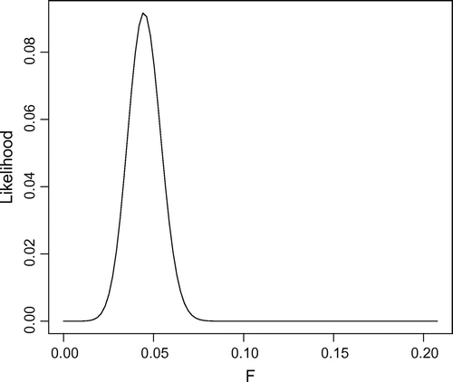
Figure 2. Likelihood contour from infile.txt using the construct function. Maximum likelihood $F_{ST}$ = 0.01 and $c_g$ = 0.55, where $R_g$ = 0.0625. Support envelope = 2e-4, which corresponds with outer most contour.

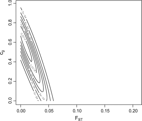
If it is suspected that the population from which these data have been collected is not a single, inbreeding population, but one that may contain subpopulations, in accordance with Wright’s island model (1931), then construct is called. construct was called as:

> construct(data="infile.txt", max.alleles=1000, f.resolution=100, c.resolution=100, r=0.0625)

The results of which are presented in Figure 2. The R output indicates that the maximum likelihood corresponds with an $F_{ST}$ = 0.01 and $c_g$ = 0.55, where $R_g$ = 0.0625. The F = 0.044 appears to be contributed to by half the population having parents related as first cousins, but also substructured into subpopulations with a variance in allele frequencies corresponding to $F_{ST}$ = 0.01.

Figure 3. Simulated data-sets where $F_{ST}$ = 0; $c_g$ = 0.5 and $R_g$ = 0.0625. Maximum likelihood values with outermost support envelope (SE): A) $c_g$=0.48; $F_{ST}$=0, SE=1e-4; B) $c_g$=0.6; $F_{ST}$=0, SE=1e-4; C) $c_g$=0.44; $F_{ST}$=0.009, SE=3e-4; D) $c_g$=0.61; $F_{ST}$=0.006, SE=1e-4; E) $c_g$=0.48; $F_{ST}$=0, SE=5e-4; F) $c_g$=0.47; $F_{ST}$=0.001, SE=1e-3.

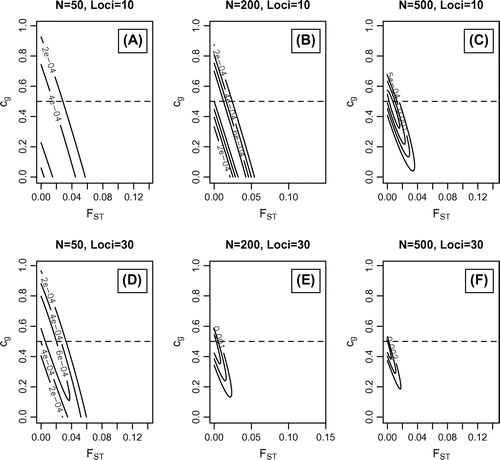
Figure 4. Simulated data-sets where $F_{ST}$ = 0.03; $c_g$ = 0.5 and $R_g$ = 0.0625. Maximum likelihood values with outermost support envelope (SE): A) $c_g$=0.41; $F_{ST}$=0.04, SE=5e-5; B) $c_g$=0.45; $F_{ST}$=0.03, SE=1e-4; C) $c_g$=0.54; $F_{ST}$=0.024, SE=2e-4; D) $c_g$=0.36; $F_{ST}$=0.023, SE=1e-4; E) $c_g$=0.59; $F_{ST}$=0.029, SE=2e-4; F) $c_g$=0.35; $F_{ST}$=0.035, SE=5e-4.

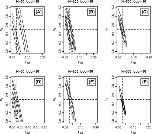
Figure 5. Simulated data-sets where $F_{ST}$ = 0.03; $c_g$ = 0 and $R_g$ = 0.0625. Maximum likelihood values with outermost support envelope (SE): A) $c_g$=0; $F_{ST}$=0.01, SE=2e-4; B) $c_g$=0; $F_{ST}$=0.03, SE=3e-4; C) $c_g$=0.03; $F_{ST}$=0.02, SE=5e-4; D) $c_g$=0.03; $F_{ST}$=0.014, SE=4e-4; E) $c_g$=0; $F_{ST}$=0.02, SE=1e-3; F) $c_g$=0; $F_{ST}$=0.03, SE=2e-3.

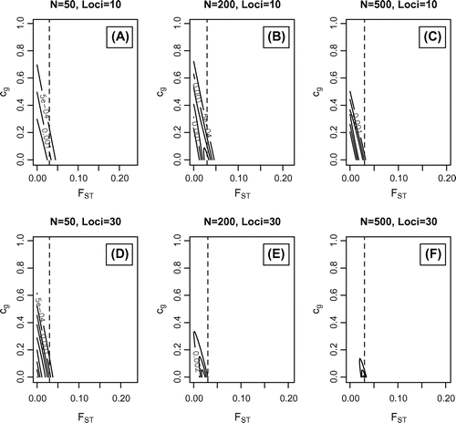
A series of scenarios were simulated by calling the simulate function to assess the performance of this method. Figure 3 presents the likelihood contours where $F_{ST}$ = 0; $c_g$ = 0.5 and $R_g$ = 0.0625. Figure 4 where $F_{ST}$ = 0.03; $c_g$ = 0.5 and $R_g$ = 0.0625 and Figure 5 where $F_{ST}$ = 0.03; $c_g$ = 0 and $R_g$ = 0.0625. All loci have eight alleles, which were specified, for example with ten loci, as num.alleles = c(8,8,8,8,8,8,8,8,8,8).

4. Discussion

Figure 1 illustrates that when a single population is analysed, the maximum likelihood estimate of F=0.44, which corresponds to homozygosity in excess of Hardy–Weinberg expectations, is broadly in agreement with a point estimate of $F_{IS}$=0.049 calculated using hierarchical F-statistics [(e.g. those employing Weir and Cockerham (1984) in GENEPOP]. Figure 2 shows the joint likelihood of $c_g$ and $F_{ST}$. The maximum value is found where $c_g$ = 0.55 and $F_{ST}$ = 0.01. The support envelope of 2e-4, which corresponds with the outermost contour of the figure, encloses parameter values that are equivalent to being significantly different from values $c_g$ = 0 and $F_{ST}$ = 0. Values that fall outside of this outermost envelope are, generally, considered to be unlikely. This additional analysis indicates that, in this example, the single parameter estimate of F=0.044 is an over-estimate of inbreeding as it is likely contributed to by cryptic substructure. Although, considering where the outermost support envelope falls, many other parameter values are, if less likely, still likely; e.g. $c_g$ = 0.2 and $F_{ST}$ = 0.03. The performance of the simulate and construct functions was assessed by generating and analysing various scenarios, presented in Figures 3–5. Both of these functions can take several minutes to execute when large population sizes and numbers of loci are considered (e.g. N = 500 and number of loci $>$ 10). Figures 3–5 illustrate that the method is able to correctly distinguish pure scenarios (Figures 3 and 5) as well as combinations of the two scenarios (Figure 4). However, the estimated range of likely parameter values can be broad with small population sizes ($<$ 200) and few loci (e.g. 10), even though the maximum likelihood values can be accurate. In addition, although eight alleles were considered here, the number and distribution of allele frequencies can be influential. Generally, rare alleles can be more informative when attempting to distinguish departures from Hardy–Weinberg equilibrium (the ratio $(p^2(1-F)+pF)/p^2$ is inversely proportional to p). It is also important to note that because the allele frequencies are estimated without consideration of sampling error, rare alleles are only expected to be reliably estimated whenever $p\&gt;10/N$ (Lynch et al., 2014). Although only a limited number of scenarios are explored here for the purpose of illustration, the performance of the method can vary depending on the allele frequency distributions and the user is encouraged to explore this influence. Analysis of more complex allele frequency distributions can be found in Overall et al. (2003) and Montarry et al. 2015.

Acknowledgements

I would like to thank Eric Petit for his suggestion to make the scripts available and Richard Nichols for his contribution to the early development of the method. I would also like to express my gratitude to the reviewers for their exceptionally helpful and instructive comments.

Additional information

Funding

The authors received no direct funding for this research.

Notes on contributors

Andrew D.J. Overall

Andy Overall has been involved in various research projects including the molecular ecology of the grey seal, Soay sheep and the hazel dormice as well as human disease genetics. His particular interest is in the roles inbreeding and population substructure play in the genetic health of populations.

References

- Clutton-Brock, T. H., Guinness, F. E., & Albon, S. D. (1982). Red deer, behaviour and ecology of two sexes. Chicago, IL: University of Chicago Press.
- Edwards, A. W. F. (1972). Likelihood. Cambridge: Cambridge University Press.
- Goudet, J. (2005). Hierfstat, a package for R to compute and test hierarchical F-statistics. Molecular Ecology Notes, 5, 184–186.
- Hamamy, H. (2012). Consanguineous marriages, preconception consultation in primary health care settings. Journal of Community Genetics, 3, 185–192.
- Hartl, D. L., & Clark, A. G. (2007). Principles of population genetics. Sunderland, MA: Sinauer.
- Hedrick, P. W. (2005). A standardized genetic differentiation measure. Evolution, 59, 1633–1638.
- Jakobsson, M., Edge, M. D., & Rosenberg, N. A. (2013). The relationship between Fst and the frequency of the most frequent allele. Genetics, 193, 515–528.
- Lynch, M., Bost, D., Wilson, S., Maruki, T., & Harrison, S. (2014). Population-genetic inference from pooled-sequencing data. Genome Biology and Evolution, 6, 1210–1218.
- Montarry, J., Jan, P. L., Gracianne, C., Overall, A. D. J., Bardou-Valette, S., Olivier, E., ... Petit, E. J. (2015). Heterozygote deficits in cyst plant-parasitic nematodes: Possible causes and consequences. Molecular Ecology, 24, 1654–1677.
- Overall, A. D. J., Ahmad, M., Thomas, M. G., & Nichols, R. A. (2003). An analysis of consanguinity and social structure within the UK Asian population using microsatellite data. Annals of Human Genetics, 67, 525–537.
- Overall, A. D. J., & Nichols, R. A. (2001). A method for distinguishing consanguinity and population substructure using multilocus genotype data. Molecular Biology and Evolution, 18, 2048–2056.
- Rousset, F. (2008). Genepop’007: A complete reimplementation of the Genepop software for windows and linux. Molecular Ecology Resources, 8, 103–106.
- Tadmouri, G. O., Nair, P., Obeid, T., Al Ali, M. T., Al Khaja, N., & Hamamy, H. (2009). Consanguinity and reproductive health among Arabs. Reproductive Health, 6, 17.
- Weir, B. S., & Cockerham, C. C. (1984). Estimating \textit{F}-statistics for the analysis of population structure. Evolution, 38, 1358–1370.
- Wright, S. (1931). Evolution in Mendelian populations. Genetics, 16, 97–159.
- Wright, S. (1951). The genetical structure of populations. Annals of Eugenics, 15, 323–354.