Improved calendar time approach for measuring long-run anomalies

Abstract

Although a large number of recent studies employ the buy-and-hold abnormal return (BHAR) methodology and the calendar time portfolio approach to investigate the long-run anomalies, each of the methods is a subject to criticisms. In this paper, we show that a recently introduced calendar time methodology, known as Standardized Calendar Time Approach (SCTA),, controls well for heteroscedasticity problem which occurs in calendar time methodology due to varying portfolio compositions. In addition, we document that SCTA has higher power than the BHAR methodology and the Fama–French three-factor model while detecting the long-run abnormal stock returns. Moreover, when investigating the long-term performance of Canadian initial public offerings, we report that the market period (i.e. the hot and cold period markets) does not have any significant impact on calendar time abnormal returns based on SCTA.

Keywords:

• long-run anomalies
• standardized abnormal returns
• test specification
• power of test

JEL classifications:

• C1
• G1

Public Interest Statement

This paper presents a methodology to analyze the aftermarket performance following IPOs, SEOs, merging and acquisition, and similar other important corporate events. While there exist conventional methods in the literature to investigate the long-run effect of corporate events on stock market performance, each approach has potential limitations. The findings of this article document that the newly developed methodology has important improvements over the traditional methods. Although the study considers the US and Canadian stock market data, this recently introduced method can be applied to other security markets as well.

1. Introduction

Two commonly used methodologies for investigating the long-term stock price performance following major corporate events are the buy-and-hold abnormal return (BHAR) approach and the calendar time portfolio (CTP) method. The BHAR is defined as the difference between the long-run holding period return of a sample firm and that of some benchmark asset. Mitchell and Stafford (2000) explain BHAR returns as the average multiyear return from a strategy of investing in all firms that complete an event and selling at the end of a pre-specified holding period versus a comparable strategy using otherwise similar nonevent firms. The calendar time method, on the other hand, is based on the mean abnormal time series returns to monthly portfolios of event firms.

Following the work of Ritter (1991), the BHAR becomes one of the most popular estimators in the literature of long-horizon event studies. A large number of papers have applied the BHAR approach in measuring long-horizon security price performance. Important examples include Barber and Lyon (1997) and Lyon, Barber, and Tsai (1999) (henceforth LBT). These studies document that an appealing feature of using the BHAR is that the buy-and-hold returns better resemble the investors’ actual investment experience than periodic (monthly) rebalancing entailed in other approaches measuring risk-adjusted performance.

Fama (1998), however, argues against the BHAR methodology because of the statistical problems associated with the use of BHAR and the relevant test statistics. He reports that the BHAR does not address the issue of potential cross-sectional correlation of event firm abnormal returns. Mitchell and Stafford (2000) also question the application of the BHAR approach suggesting that the assumption of independence of observations is violated and hence the cross-sectional correlations significantly bias the test statistics that are computed from the BHARs. In addition, Eckbo, Masulis, and Norli (2000) document that the BHAR methodology is not a feasible portfolio strategy because the total number of stocks is not known in advance. As an alternative, the CTP approach, developed by Jaffe (1974) and Mandelker (1974), is widely used to resolve the issue of cross-sectional dependence of abnormal returns (Fama, 1998; Mitchell & Stafford, 2000). Fama (1998) strongly recommends the use of the CTP methodology on the grounds that monthly returns are less susceptible to the bad model problem as they are less skewed and by forming monthly CTPs, all cross correlations of event firm abnormal returns are automatically accounted for in the portfolio variance. Fama also documents that the distribution of this estimator is better approximated by the normal distribution, allowing for classical statistical inference. Mitchell and Stafford (2000), like Fama (1998), also prefer the CTP approach to the BHAR methodology as the latter assumes independence of multi-year event-firm abnormal returns.

While many recent studies strongly advocate the CTP approach, it has a number of potential pitfalls. For example, if there is a differential abnormal performance in periods of heavy event activity versus periods of light event activity, the regression approach will average over these, and it may be less likely to identify the abnormal performance. Loughran and Ritter (2000) argue that corporate executives time the events to exploit mispricing, but the CTP approach, by forming calendar-time portfolios, under-weights managers’ timing decisions and over-weights other observations. Since the CTP approach weights each period equally, it has lower power to detect abnormal performance if managers time corporate events to coincide with misvaluations. LBT, however, claim that the CTP approach is misspecified in nonrandom samples, while the BHAR approach is relatively robust. Finally, the CTP approach suffers from heteroscedasticity problem which occurs due to varying portfolio composition.

In this paper, we document that the standardized calendar time approach (SCTA), proposed by Dutta (2014a), alleviates these concerns to some extent. Our major contributions to the literature are the following. First, our analysis shows that SCTA documents better power than the conventional methods. Second, weighting the monthly portfolios such that periods of high event activity receive more loadings than that of low event activity, SCTA reports the issue of hot and cold period activities. However, we investigate the long-term aftermarket performance of Canadian initial public offering (IPO) stocks to address the latter issue. Third, SCTA is well specified in nonrandom samples. Finally, we prove that SCTA controls well for heteroscedasticity problem.

The present study differs from Dutta (2014a) in several ways. First, we show that SCTA mitigates the heteroscedasticity problem. Second, we demonstrate the effect of hot and cold market activities on the calendar time abnormal returns. Third, Dutta does not consider the value-weighted portfolios in his empirical analysis. Finally, Dutta does not investigate any asset pricing models for assessing the robustness of his results.

The rest of the paper will proceed as follows. Section 2 summarizes the data and methodologies. The simulation design is explained in Section 3. Section 4 presents the specification of the tests and the analysis of the Canadian IPO performance. Section 5 reports the power of the tests. Section 6 concludes the paper.

2. Data and methodology

The data used in this paper consist of NYSE, Amex, and Nasdaq stocks, and our sample period ranges from July 1978 to December 2007. We obtain monthly returns, market value (MV) or size, and book-to-market (BM) value data from Datastream.

We construct 25 size-BM portfolios as expected return benchmarks. In doing so, at the end of June of year t, we allocate all the stocks to one of five size groups, based on size rankings relative to NYSE quintiles. In an independent sort, all stocks are also allocated to one of five BM groups based on their BM ranks relative to NYSE quintiles.

2.1. Standardized calendar time approach

The conventional way of calculating the mean monthly calendar time abnormal return (CTAR) is the following(1) $$\begin{array}{c}\hfill \text{mean monthly CTAR}=\frac{1}{T}\sum _{t=1}^T{\text{CTAR}}_t,\end{array}$$(1)

where(2) $$\begin{array}{c}\hfill {\mathrm{CTAR}}_t=R_{pt}-E(R_{pt}),\end{array}$$(2)

Within this framework, $R_{pt}$ is the monthly return on the portfolio of event firms, $E(R_{pt})$ is the expected return on the event portfolio which is proxied by the raw return on a reference portfolio, and T is the total number of months in the sample period.

However, a number of firms in the sample often produce volatile returns. Small firms, for instance, usually exhibit such pattern and because of this volatility, the distributions of long-run returns tend to have fat tails. But one possible solution to this problem is standardizing the abnormal returns by their volatility measures. In this paper, we use standardized abnormal returns to compute the CTARs. The whole procedure is done in two steps (Dutta, 2014a). We first calculate the standardized abnormal returns for each of the sample firms. In doing so, the abnormal return for a firm i is computed as ${\mathit{\epsilon }}_{it}=R_{it}-E(R_{it});t=1,\dots ,H$, where $R_{it}$ denotes the return on event firm i in the calendar month t, $E(R_{it})$ is the expected return on the event portfolio which is proxied by 25 size-BM reference portfolios, and H is the holding period which equals 12, 36, or 60 months. The next task is to estimate the event-portfolio residual variances using the H-month residuals computed as monthly differences of ith event firm returns and size-BM portfolio returns. Dividing ${\mathit{\epsilon }}_{it}$ by the estimate of its standard deviation yields the corresponding standardized abnormal return, say $z_{it}$, for event firm i in month t. Now, let $N_t$ refer to the number of event firms in the calendar month t. We then calculate the calendar time abnormal return for portfolio t as(3) $$\begin{array}{c}\hfill {\text{CTAR}}_t=\sum _{i=1}^{N_t}{x}_{it}{z}_{it},\end{array}$$(3)

where the weight $x_{it}$ equals $\frac{1}{N_t}$ when the abnormal returns are equally weighted and $\frac{{\mathrm{MV}}_{\mathrm{it}}}{\sum {\mathrm{MV}}_{\mathrm{it}}}$ when the abnormal returns are value-weighted by size.

Following Dutta (2014b), we also weight each of the monthly CTARs by $\frac{1}{\sqrt{(}{\sum }_{i=1}^{N_t}{x}_{it}^2)}$. For instance, when the abnormal returns are equally weighted i.e. when $x_{it}=\frac{1}{N_t}$, then $\frac{1}{\sqrt{(}{\sum }_{i=1}^{N_t}{x}_{it}^2)}={\sqrt{N}}_t$. This weighting scheme is lucrative as it gives more loadings to periods of heavy event activity than the periods of low event activity. Now, the grand mean monthly abnormal return ($\overline{\text{CTAR}}$) is calculated as(4) $$\begin{array}{c}\hfill \overline{\text{CTAR}}=\frac{1}{T}\sum _{t=1}^T{\text{CTAR}}_t\end{array}$$(4)

While finding $\overline{\mathrm{CTAR}}$, it might be the case that a number of portfolios do not contain any event firm. In such situations, those months are dropped from the analysis. To test the null hypothesis that there is no abnormal performance, the t-statistic of $\overline{\mathrm{CTAR}}$ is computed using the intertemporal standard deviation of the monthly CTARs defined in Equation 3.

However, since the number of event firms in the CTP approach does vary over the sample period, this may introduce heteroscedasticity. Thus, how to alleviate this heteroscedasticity problem becomes an important statistical issue. We now show that SCTA solves this problem by producing constant variances for all the weighted portfolios over the sample period.

For simplicity, let $x_{it}=\frac{1}{N_t}$. Then, the variance of portfolio t is$$\begin{array}{cc}\hfill Var({\sqrt{N}}_t{\mathrm{CTAR}}_t)& =N_{t}Var({\mathrm{CTAR}}_t)\hfill \\ \hfill & =N_{t}Var(\frac{1}{N_t}\sum _{i=1}^{N_t}{z}_{it})+N_t\sum _{i\ne j}\frac{1}{N_t}\frac{1}{N_t}cov(z_{it},z_{jt})\hfill \\ \hfill & =\frac{N_t}{N_t^2}\sum _{i=1}^{N_t}Var(z_{it})+\frac{1}{N_t}\sum _{i\ne j}{\mathit{\rho }}_{ijt}\hfill \\ \hfill & =\frac{N_t}{N_t}+\frac{1}{N_t}\sum _{i\ne j}{\mathit{\rho }}_{ijt}\hfill \\ \hfill & [\text{Since the variance of standardized abnormal return is}\text{1}.]\hfill \\ \hfill & =1+\frac{1}{N_t}\sum _{i\ne j}{\mathit{\rho }}_{ijt}\hfill \\ \hfill & =1+(N_t-1)\overline{{\mathit{\rho }}_t}\hfill \end{array}$$

where $\overline{{\mathit{\rho }}_t}$ refers to the average cross-sectional correlation for portfolio t. However, in practice, $\overline{{\mathit{\rho }}_t}$ is a small quantity. Now, if the number of firms in the portfolios does not vary significantly, the variance is likely to behave as a constant. We, therefore, document that SCTA yields a convenient solution to the heteroscedasticity problem.

2.2. Buy-and-hold abnormal return

Once a reference portfolio is identified, computing BHARs is straightforward. A H-month BHAR for event firm i is defined as(5) $$\begin{array}{c}\hfill {\mathrm{BHAR}}_{iH}=\prod _{t=1}^H(1+R_{it})-\prod _{t=1}^H(1+R_{Bt}),\end{array}$$(5)

where $R_{it}$ denotes the return on event firm i at time t and $R_B$ indicates the return on 25 size-BM reference portfolios.

To test the null hypothesis that the mean buy-and-hold return equals zero, the conventional t-statistic is given by(6) $$\begin{array}{c}\hfill t_{\mathrm{BHAR}}=\frac{\overline{{\mathrm{BHAR}}_H}}{\mathit{\sigma }({\mathrm{BHAR}}_H)/\sqrt{n}},\end{array}$$(6)

where $\overline{{\mathrm{BHAR}}_H}$ implies the sample mean and $\mathit{\sigma }({\mathrm{BHAR}}_H)$ refers to the cross-sectional sample standard deviation of abnormal returns for the sample containing n firms.

However, the earlier studies (e.g. Boehme & Sorescu, 2002; Jegadeesh & Karceski, 2009; Mitchell & Stafford, 2000) report that the BHAR approach does not control well for the cross-sectional correlation among individual firms in nonrandom s amples, and thus yields misspecified t-statistics. Moreover, the test statistics based on BHARs also suffers from this misspecification problem due to the severe skewness of the distribution of BHARs. Though bootstrapping corrects the skewness problem to some extent, it ignores the cross-sectional dependence of abnormal returns.

2.3. Fama–French three-factor model

For completeness, we also report the results from the Fama–French three-factor model. For each calendar month t, we form portfolios consisting of all sample firms that have participated in the event within the last H months, where H equals 12, 36, or 60 in our study. For each calendar month, the portfolios are rebalanced, i.e. the firms that reach the end of their H-month period drop out and new firms that have just executed a transaction are added. We then calculate the portfolio mean monthly abnormal return ${\mathit{\alpha }}_p$ by regressing its excess return on the three Fama–French factors(7) $$\begin{array}{c}\hfill R_{pt}-R_{ft}={\mathit{\alpha }}_p+{\mathit{\beta }}_p(R_{mt}-R_{ft})+s_{p}SM{B}_t+h_{p}HM{L}_t+e_{pt},\end{array}$$(7)

where $R_{pt}$ is the equal or value-weighted return on portfolio t, $R_{ft}$ is the risk-free rate, $R_{mt}-R_{ft}$ is the excess return of the market, SMB is the difference between the return on the portfolio of small stocks and big stocks, HML is the difference between the return on the portfolio of high and low BM stocks, ${\mathit{\alpha }}_p$ measures the mean monthly abnormal return of the CTP which is zero under the null hypothesis of no abnormal performance, and ${\mathit{\beta }}_p$, $s_p$, and $h_p$ are sensitivities of the event portfolio to the three factors.

However, since the number of firms changes over the sample period, this may cause the error term to be heteroskedastic, and hence the ordinary least squares estimate becomes inefficient. Fama (1998), therefore, suggests applying the weighted least squares technique instead of ordinary least squares to control for heteroscedasticity. In this study, we estimate regression (7) using weighted least squares (WLS) procedures. Monthly returns in the WLS model are weighted by $\sqrt{N_t}$, where $N_t$ stands for the number of event firms in month t.

3. Simulation method

To test the specification of the t-statistics, we randomly select 1,000 samples of 200 event months without replacement. For each of these 200 event months, we randomly draw one stock from the population of all stocks that are active in the database for that month. For a well-specified test statistic, 1000$\mathit{\alpha }$ tests reject the null hypothesis. A test is conservative if fewer than 1000$\mathit{\alpha }$ null hypotheses are rejected and is anticonservative if more than 1000$\mathit{\alpha }$ null hypotheses are rejected. Based on this procedure, we test the specification of the t-statistic at 5% theoretical levels of significance. A well-specified null hypothesis rejects the null at the theoretical rejection level in favor of the alternative hypothesis of negative (positive) abnormal returns in 1,000$\mathit{\alpha }/2$ samples.

4. Test specification

This section reports the specification of various methodologies used in our study. We first discuss the results in random samples. Later, we consider different types of nonrandom samples based on firm size, BM ratio, pre-event return performance, and overlapping returns.

4.1. Random samples

Table 1A indicates the rejection rates in 1,000 simulations with a random sample of 200 firms. Findings reveal that all the t-statistics based on buy-and-hold abnormal returns are negatively biased. For example, when the horizons are five years, the rejection rates at the 5% level of significance are 4.8 and 0%. These results are consistent with those documented by LBT, where the tests have higher rejection rates in the lower tail.

As anticipated, all the CTP methods considered in our analysis are well specified in random samples regardless of whether equally weighted or value-weighted portfolios are employed. For example, for a three-year holding period with equally weighted portfolios, the rejection rates at 5% level of significance are 2.4 and 2.8% and 2 and 0.8% for the t-statistics produced by the SCTA and Fama–French three-factor model, respectively.

Table 1. Specification of tests in random samples

Method description	1 Year		3 Years		5 Years
	2.5	97.5	2.5	97.5	2.5	97.5
Panel A: Equally weighted portfolios
Standardized calendar time approach	1.2	2.8	2.4	2.8	1.2	2.4
Buy-and-hold abnormal return method	6.2^*	0.8	4.4^*	0.4	4.8^*	0.0
Fama–French three-factor model	4.4^*	0.8	2.0	0.8	3.2	1.6
Panel B: Value-weighted portfolios
Standardized calendar time approach	1.6	2.4	1.2	3.2	1.2	3.4
Fama–French three-factor model	3.6	1.2	2.0	2.0	0.8	2.8

Notes: This table presents the percentages of 1,000 random samples of 200 firms that reject the null hypothesis of no abnormal returns over one-year, three-year, and five-year holding periods at the theoretical significance level of 5% in favor of the alternative hypothesis of a significantly negative intercept (i.e. calculated $p$ value is less than 2.5 at the 5% significance level) or a significantly positive intercept (calculated $p$ value is greater than 97.5% at the 5% significance level).

* Empirical size is significantly different from the 5% significance level. We, however, employ 25 size-BM reference portfolios to measure the BHARs and CTARs.

However, our proposed calendar time approach involves two components: standardization and weighting. In order to verify whether it is the standardization or the weighting approach that improves the specification of tests, the table presents a set of simulation results for the following cases: (a) standardization only approach and (b) weighting only approach. Table 1B shows that the standardization only approach produces well-specified test statistics when the length of the investment periods is either three or five years. But, for a one-year horizon, there is some evidence of misspecification. For the weighting only approach, we document misspecifications when the holding periods are one year and five years. Similar comments also apply when the portfolios are value weighted. Hence, we conclude that the SCTA, which involves both standardization and weighting components, improves the size of tests as shown in Table 1A.

Table 2. Specification of tests in random samples

Method description	1 Year		3 Years		5 Years
	2.5	97.5	2.5	97.5	2.5	97.5
Panel A: Equally weighted portfolios
Standardization only approach	1.3	8.3^*	2.0	3.2	3.4	2.8
Weighting only approach	5.6^*	0.4	2.0	3.0	1.1	4.2^*
Panel B: Value-weighted portfolios
Standardization only approach	0.2	4.0^*	1.6	2.7	4.1^*	2.3
Weighting only approach	3.8^*	2.6	1.2	3.1	0.3	5.8^*

Notes: This table reports the results from standardization only approach and weighting only approach. The standardization only approach does not weight the monthly portfolios, while the weighting only approach does not standardize the event firm anomalies. The numbers shown in this table present the percentages of 1,000 random samples of 200 firms that reject the null hypothesis of no abnormal returns over one-year, three-year, and five-year holding periods at the theoretical significance level of 5% in favor of the alternative hypothesis of a significantly negative intercept (i.e. calculated $p$ value is less than 2.5% at the 5% significance level) or a significantly positive intercept (calculated $p$ value is greater than 97.5% at the 5% significance level).

* Empirical size is significantly different from the 5% significance level.

Table 3. Regression analysis of hot and cold markets

Periods	EW porfolios	VW portfolios
Hot period	0.12 (0.79)	0.08 (1.19)
Cold period	0.23 (-0.91)	0.14 (0.31)

Notes: This table presents the effect of hot and cold markets on CTAR obtained from SCTA over a three-year horizon. EW and VW portfolios indicate equally and value-weighted portfolios, respectively. The values in the parentheses report the t-statistics.

Table 4. Specification of tests in samples with large firms

Method description	1 Year		3 Years		5 Years
	2.5	97.5	2.5	97.5	2.5	97.5
Panel A: Equally weighted portfolios
Standardized calendar time approach	0.4	4.8^*	0.8	2.0	1.6	2.0
Buy-and-hold abnormal return method	0.0	16.8^*	0.0	18.8^*	0.0	22.0^*
Fama–French three-factor model	0.8	4.0^*	1.6	2.8	2.8	2.0
Panel B: Value-weighted portfolios
Standardized calendar time approach	0.0	4.0^*	0.8	2.4	1.6	3.4
Fama–French three-factor model	0.8	4.8^*	0.8	2.8	2.8	2.4

Notes: This table presents the percentages of 1,000 samples of 200 large firms that reject the null hypothesis of no abnormal returns over one-year, three-year, and five-year holding periods at the theoretical significance level of 5% in favor of the alternative hypothesis of a significantly negative intercept (i.e. calculated $p$ value is less than 2.5% at the 5% significance level) or a significantly positive intercept (calculated $p$ value is greater than 97.5% at the 5% significance level).

* Empirical size is significantly different from the 5% significance level.

Table 5. Specification of tests in samples with small firms

Method description	1 Year		3 Years		5 Years
	2.5	97.5	2.5	97.5	2.5	97.5
Panel A: Equally weighted portfolios
Standardized calendar time approach	4.0^*	0.8	2.4	1.6	1.6	3.6
Buy-and-hold abnormal return method	24.6^*	0.0	9.2^*	0.0	9.2^*	0.0
Fama–French three-factor model	6.2^*	0.8	4.4^*	1.6	2.4	2.4
Panel B: Value-weighted portfolios
Standardized calendar time approach	4.6^*	2.4	3.2	2.4	0.4	2.8
Fama–French three-factor model	4.0^*	1.8	2.8	2.4	0.8	4.4^*

Notes: This table presents the percentages of 1,000 samples of 200 small firms that reject the null hypothesis of no abnormal returns over one-year, three-year, and five-year holding periods at the theoretical significance level of 5% in favor of the alternative hypothesis of a significantly negative intercept (i.e. calculated $p$ value is less than 2.5% at the 5% significance level) or a significantly positive intercept (calculated $p$ value is greater than 97.5% at the 5% significance level).

* Empirical size is significantly different from the 5% significance level.

Moreover, in order to examine whether the hot and cold event activity periods have any impact on the CTARs based on SCTA, we consider investigating the long-run performance of Canadian IPOs. Our sample contains 130 IPOs issued by the Toronto Stock Exchange firms during the period from 1990 to 1999. We construct 25 size-BM reference portfolios to measure the CTARs over a three-year window. We consider CTAR as the dependent variable and hot market along with cold market as the regressors. We follow Mitchell and Stafford (2000) to define the hot and cold market variables. The hot market variable equals 1 if event activity lies above the 70th percentile of all monthly activities and 0 otherwise. The cold market variable, on the other hand, takes the value 1 if event activity lies below the 30th percentile of all monthly activities and 0 otherwise. Moreover, the monthly activity is defined as the number of firms in the event portfolio divided by the total number of firms in the corresponding month. Our analysis shows that the t-statistics reported in Table 1C are not statistically significant, implying that the hot as well as the cold markets do not influence the CTARs based on SCTA. We, therefore, conclude that the abnormal performance is not concentrated in periods when there are relatively large number of events.

4.2. Nonrandom samples

4.2.1. Firm size

In order to investigate the effect of size-based sampling biases on the employed methods, we randomly choose 1,000 samples separately from the largest size decile and smallest size decile. These results are presented in Tables 2A and 2B. Our analysis indicates that among the three methods, SCTA is better specified for each type of samples based on size. For instance, for a five-year horizon and with small firms and value-weighted portfolios, the rejection rates at 5% level of significance are 0.4 and 2.8% for the SCTA and 0.8 and 4.4% for the FF3F model. However, the t-statistics based on the BHAR approach are negatively skewed for samples containing small firms and positively skewed for samples consisting large firms.

4.2.2. Book-to-market ratio

Firms are deciled into 10 groups based on rankings of the BM ratio at the end of June, each year. We choose the groups with the highest BM ratio and the lowest BM ratio for robustness check. For each group, we select a random sample of 200 firms. The procedure is repeated 1,000 times and Tables 3A and 3B report the rejection rates. Inspection of these tables suggests that the standardized CTP approach yields reasonably well-specified test statistics in each case. For example, for a three-year holding period with equally weighted portfolios and firms with low BM ratio, the rejection rates at 5% level of significance are 1.6 and 2.0% for the SCTA and 0.2 and 5.6% for the FF3F model. The BHAR method, on the other hand, produces either negatively or positively skewed test statistics depending on low or high BM value, respectively.

Table 6. Specification of tests in samples of firms with high BM value

Method description	1 Year		3 Years		5 Years
	2.5	97.5	2.5	97.5	2.5	97.5
Panel A: Equally weighted portfolios
Standardized calendar time approach	2.0	3.2	1.6	2.0	0.0	6.0^*
Buy-and-hold abnormal return method	0.0	32.2^*	0.0	29.2^*	0.1	17.8^*
Fama–French three-factor model	0.4	7.2^*	0.2	5.6^*	0.8	3.6
Panel B: Value-weighted portfolios
Standardized calendar time approach	1.2	3.2	1.2	2.4	0.0	4.0^*
Fama–French three-factor model	0.0	10.1^*	0.4	5.4^*	0.8	5.6^*

Notes: This table presents the percentages of 1,000 samples of 200 firms with high BM value that reject the null hypothesis of no abnormal returns over one-year, three-year, and five-year holding periods at the theoretical significance level of 5% in favor of the alternative hypothesis of a significantly negative intercept (i.e. calculated $p$ value is less than 2.5% at the 5% significance level) or a significantly positive intercept (calculated $p$ value is greater than 97.5% at the 5% significance level).

* Empirical size is significantly different from the 5% significance level.

Table 7. Specification of tests in samples of firms with low BM value

Method description	1 Year		3 Years		5 Years
	2.5	97.5	2.5	97.5	2.5	97.5
Panel A: Equally weighted portfolios
Standardized calendar time approach	2.8	2.4	1.6	0.4	2.0	0.4
Buy-and-hold abnormal return method	14.0^*	0.0	10.4^*	0.2	8.2^*	0.0
Fama–French three-factor model	14.0^*	0.0	8.8^*	0.4	6.8^*	0.0
Panel B: Value-weighted portfolios
Standardized calendar time approach	1.6	2.4	2.4	0.8	1.2	0.4
Fama–French Three-Factor Model	11.0^*	0.0	6.0^*	0.8	4.0^*	0.0

Notes: This table presents the percentages of 1,000 samples of 200 firms with low BM value that reject the null hypothesis of no abnormal returns over one-year, three-year, and five-year holding periods at the theoretical significance level of 5% in favor of the alternative hypothesis of a significantly negative intercept (i.e. calculated $p$ value is less than 2.5% at the 5% significance level) or a significantly positive intercept (calculated $p$ value is greater than 97.5% at the 5% significance level).

* Empirical size is significantly different from the 5% significance level.

4.2.3. Pre-event return performance

To assess the specification of the tests under study, we consider drawing firms on the basis of pre-event return performance. Following LBT, we compute the preceding six-month buy-and-hold return on all firms in each month from July 1978 to December 2012. We then decile this six-month return and separately select 1,000 samples of 200 firms from the high-return decile and the low-return decile. The findings of our analysis are shown in Tables 4A and 4B.

Table 8. Specification of tests in samples with good pre-event returns: Case I

Method description	1 Year		3 Years		5 Years
	2.5	97.5	2.5	97.5	2.5	97.5
Panel A: Equally weighted portfolios
Standardized calendar time approach	0.4	9.2^*	2.0	4.0^*	1.2	4.8^*
Buy-and-hold abnormal return method	0.0	6.8^*	14.0^*	0.2	21.4^*	1.6
Fama–French three-factor model	0.4	8.0^*	3.2	2.8	3.2	1.2
Panel B: Value-weighted portfolios
Standardized calendar time approach	0.0	12.0^*	1.2	3.6	0.4	4.8^*
Fama–French three-factor model	0.4	10.0^*	2.0	5.2^*	2.4	4.6^*

Notes: This table presents the percentages of 1,000 samples of 200 firms with good pre-event returns that reject the null hypothesis of no abnormal returns over one-year, three-year, and five-year holding periods at the theoretical significance level of 5% in favor of the alternative hypothesis of a significantly negative intercept (i.e. calculated $p$ value is less than 2.5% at the 5% significance level) or a significantly positive intercept (calculated $p$ value is greater than 97.5% at the 5% significance level).

* Empirical size is significantly different from the 5% significance level. We, however, employ 25 size-BM reference portfolios to measure the BHARs and CTARs.

Table 9. Specification of tests in samples with poor pre-event returns: Case I

Method description	1 Year		3 Years		5 Years
	2.5	97.5	2.5	97.5	2.5	97.5
Panel A: Equally weighted portfolios
Standardized calendar time approach	14.0^*	0.4	0.4	2.8	1.2	1.6
Buy-and-hold abnormal return method	21.2^*	0.0	8.4^*	0.1	4.6^*	0.3
Fama–French three-factor model	16.8^*	0.0	2.6	4.2^*	2.1	2.0
Panel B: Value-weighted portfolios
Standardized calendar time approach	6.8^*	0.4	0.4	4.0^*	0.8	4.0^*
Fama–French three-factor model	9.6^*	0.4	0.6	2.4	0.4	2.8

Notes: This table presents the percentages of 1,000 samples of 200 firms with poor pre-event returns that reject the null hypothesis of no abnormal returns over one-year, three-year, and five-year holding periods at the theoretical significance level of 5% in favor of the alternative hypothesis of a significantly negative intercept (i.e. calculated $p$ value is less than 2.5% at the 5% significance level) or a significantly positive intercept (calculated $p$ value is greater than 97.5% at the 5% significance level).

* Empirical size is significantly different from the 5% significance level. We, however, employ 25 size-BM reference portfolios to measure the BHARs and CTARs.

Table 10. Specification of tests in samples with good pre-event returns: Case II

Method description	1 Year		3 Years		5 Years
	2.5	97.5	2.5	97.5	2.5	97.5
Panel A: Equally weighted portfolios
Standardized calendar time approach	0.3	4.6^*	3.1	3.6	2.4	0.7
Buy-and-hold abnormal return method	0.2	4.2^*	3.8^*	2.3	3.0	1.1
Carhart four-factor model	0.0	5.6^*	2.3	2.4	0.9	3.1
Panel B: Value-weighted portfolios
Standardized calendar time approach	2.8	4.0^*	1.8	3.4	3.6	2.1
Carhart four-factor model	0.4	3.8^*	2.6	1.9	2.9	3.6

Notes: This table presents the percentages of 1,000 samples of 200 firms with good pre-event returns that reject the null hypothesis of no abnormal returns over one-year, three-year, and five-year holding periods at the theoretical significance level of 5% in favor of the alternative hypothesis of a significantly negative intercept (i.e. calculated $p$ value is less than 2.5% at the 5% significance level) or a significantly positive intercept (calculated $p$ value is greater than 97.5% at the 5% significance level). However, the difference between this table and Table 4A is that here we employ $5\times 5\times 5$ size-BM-past returns reference portfolios to measure the BHARs and CTARs. We also estimate the four-factor model of Carhart (1997) to include the momentum factor computed as the difference between returns of winners and losers. We, therefore, exclude the three-factor model while constructing Table 4C.

* Empirical size is significantly different from the 5% significance level.

Table 11. Specification of tests in samples with poor pre-event returns: Case II

Method description	1 Year		3 Years		5 Years
	2.5	97.5	2.5	97.5	2.5	97.5
Panel A: Equally weighted portfolios
Standardized calendar time approach	3.7^*	1.6	2.8	2.0	3.5	1.3
Buy-and-hold abnormal return method	4.8^*	1.2	3.6	2.7	2.6	2.2
Carhart four-factor model	4.4^*	0.3	3.7^*	1.9	2.3	1.6
Panel B: Value-weighted portfolios
Standardized calendar time approach	4.1^*	2.1	2.6	0.3	3.4	2.0
Carhart four-factor model	3.8^*	0.2	1.1	2.3	3.6	2.7

Notes: This table presents the percentages of 1,000 samples of 200 firms with poor pre-event returns that reject the null hypothesis of no abnormal returns over one-year, three-year, and five-year holding periods at the theoretical significance level of 5% in favor of the alternative hypothesis of a significantly negative intercept (i.e. calculated $p$ value is less than 2.5% at the 5% significance level) or a significantly positive intercept (calculated $p$ value is greater than 97.5% at the 5% significance level). However, the difference between this table and Table 4B is that here we employ $5\times 5\times 5$ size-BM-past returns reference portfolios to measure the BHARs and CTARs. We also estimate the four-factor model of Carhart (1997) to include the momentum factor computed as the difference between the returns of winners and losers. We, therefore, exclude the three-factor model while constructing Table 4D.

* Empirical size is significantly different from the 5% significance level.

Scrutinizing these two tables suggests that most of the tests produce either positively or negatively biased test statistics and these results resemble those of LBT. Jegadeesh and Titman (1993), however, also report similar types of findings. LBT, however, suggests to match sample firms with firms of similar pre-event return performance to avoid this type of misspecification. Following LBT, we construct $5\times 5\times 5$ reference portfolios based on size, BM, and pre-event return performance. Simulated results, shown in Tables 4C and 4D, report that the level of specification of the methods considered improves. We employ the four-factor model, proposed by Carhart (1997), to include the momentum factor computed as the difference between returns of winners and losers. We, therefore, exclude the three-factor model while constructing Tables 4C and 4D. Unfortunately, such portfolios are not equally effective (not reported in the table) when analyzing random samples as well as other nonrandom samples.

4.2.4. Overlapping returns

With a view to inspecting how the methods used in this paper behave in the presence of cross-sectional correlation of abnormal returns, we consider nonrandom samples based on overlapping returns. Selecting these samples consists of two steps. The first stage involves a random selection of 100 firms from the population. In the second stage, for each of these 100 firms, we randomly choose a second event month that is within $H-1$ periods of the original event month (either before or after), where H equals 12, 36, or 60. Hence, we have 200 firms with 200 event months, where the same firm appears in the sample twice and this generates the issue of overlapping returns. We repeat this procedure 1,000 times and the results are presented in Table 5.

Findings indicate that the BHAR approach yields misspecified test statistics and these results are consistent with those reported in previous studies (e.g. Lyon et al., 1999; Mitchell & Stafford, 2000). This misspecification is due to the fact that BHAR assumes that the observations are cross sectionally uncorrelated. This assumption is tenable in random samples of event firms, but it would be violated in nonrandom samples, where the returns for event firms are positively correlated (Jegadeesh & Karceski, 2009).

Table 12. Specification of tests in samples with overlapping returns

Method description	1 Year		3 Years		5 Years
	2.5	97.5	2.5	97.5	2.5	97.5
Panel A: Equally weighted portfolios
Standardized calendar time approach	3.2	2.0	2.9	3.6	2.4	3.2
Buy-and-hold abnormal return method	7.2^*	0.4	9.4^*	3.6	10.2^*	4.8^*
Fama–French three-factor model	1.2	1.6	2.3	2.4	2.8	2.1
Panel B: Value-weighted portfolios
Standardized calendar time approach	3.2	1.6	1.8	3.1	1.6	2.0
Fama–French three-factor model	2.8	0.8	1.6	3.4	2.2	3.3

Notes: This table presents the percentages of 1,000 samples of 200 firms with overlapping returns that reject the null hypothesis of no abnormal returns over one-year, three-year, and five-year holding periods at the theoretical significance level of 5% in favor of the alternative hypothesis of a significantly negative intercept (i.e. calculated $p$ value is less than 2.5% at the 5% significance level) or a significantly positive intercept (calculated $p$ value is greater than 97.5% at the 5% significance level). Selecting these samples is a two-step procedure. The first step involves a random selection of 100 firms from the population. In the second step, for each of these 100 firms, we randomly choose a second event month that is within $H-1$ periods of the original event month (either before or after), where H equals 12, 36, or 60. Hence, we have 200 firms with 200 event months, where the same firm appears in the sample twice and this generates the issue of overlapping returns. We repeat this procedure 1,000 times.

* Empirical size is significantly different from the 5% significance level.

Results further confirm that each of the calendar time methods performs well when return calculations do overlap. In most of the cases, the equally weighted scheme produces higher rejection compared with the value-weighted scheme. For example, for a three-year holding period with equally weighted portfolios, the rejection rates at 5% level of significance are 2.9 and 3.6% for the t-statistics produced by SCTA. The corresponding rejection rates are 1.8 and 3.1% when the portfolios are value weighted. It indicates that the value-weighted scheme should be taken into account if misspecifications occur due to overlapping returns. Last but not the least, the CTP approach controls well for the problem of cross-sectional dependence and is thus recommended while dealing with cross-sectionally correlated returns.

5. Power

In this section, we compare the power of all the three methods employed in our study. Note that we only choose random samples since the t-tests are not, in general, well specified in nonrandom samples. To examine the power of test, we introduce a constant level of abnormal return ranging from –20 to 20% at an interval of 5% to event firms. We also consider equally weighted portfolios to make a direct comparison with the BHAR approach. Table 6 indicates the percentages of 1,000 samples of 200 firms that reject the null hypothesis of zero abnormal returns over a three-year holding period. Figure 1 also plots power of the tests.

Figure 1. Simulated power of different methods in random samples. Notes: This figure represents the percentages of 1,000 random samples of 200 firms that reject the null hypothesis of no abnormal returns over three-year holding period. We consider equally weighted portfolios to make a direct comparison with the BHAR approach. The horizontal axis indicates the induced level of abnormal returns (%), while the rejection rates are shown in the vertical axis.

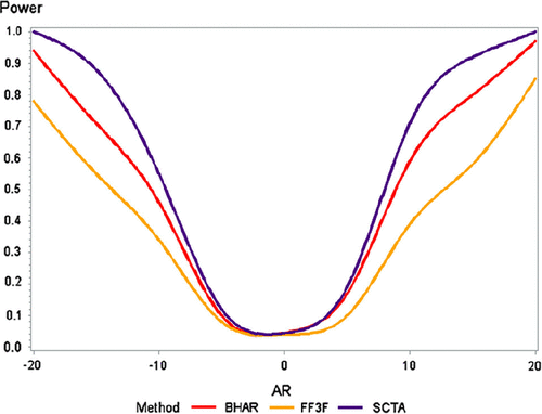
Table 13. Power of alternative methods in random samples

Method description	Induced level of abnormal return (%) over 3 years
	–20	–15	–10	–5	0	5	10	15	20
Standardized calendar time approach	1.00	0.88	0.56	0.11	0.05	0.18	0.71	0.92	1.00
Buy-and-hold abnormal return method	0.94	0.71	0.46	0.11	0.05	0.17	0.59	0.80	0.97
Fama–French three-factor model	0.78	0.55	0.34	0.08	0.04	0.10	0.39	0.58	0.85

Notes: This table presents the percentages of 1,000 random samples of 200 firms that reject the null hypothesis of no abnormal returns over a three-year holding period. We add the levels of annual abnormal return indicated in the column heading. However, only equally weighted portfolios are considered to make a direct comparison with the BHAR approach.

It is evident from Table 6 and Figure 1 that our proposed SCTA produces the most powerful t-statistic, followed by the BHAR method, and the test statistic based on the Fama–French three-factor model is the least powerful. For instance, with 15% per year abnormal returns, the rejection rate is 92% for the SCTA, 80% for the BHAR method, and 58% for the FF3F model. We, therefore, conclude that the SCTA produces more power to detect the abnormal performance than the BHAR method, after accounting for cross-sectional correlation of the event firms.

6. Conclusion

The proper methodology for analyzing the long-term return anomalies has been much debated in the literature. Kothari and Warner (2007), for instance, report that the question of which model of expected returns is correct remains an unresolved issue. Fama (1998) also concludes that not a single model for expected returns can fully describe the systematic patterns in normal returns, and hence the anomalies arise because of the misspecification of models and the statistical tests applied. A fundamental choice for many recent studies, therefore, concerns the measure of the long-run stock price performance.

Although numerous event studies have employed the BHAR methodology and the CTP approach for investigating the long-run abnormal performance, each method has serious limitations. For example, Mitchell and Stafford (2000) argue against using the BHAR methodology as it assumes event firm abnormal returns to be independent. They argue that major corporate actions are not random events, and thus event samples are likely to consist of dependent observations. In particular, major corporate events cluster through time by an industry. This leads to a positive cross correlation of abnormal returns, making test statistics that assume independence severely overstated. They, like Fama (1998), strongly recommend the use of the CTP approach. Loughran and Ritter (2000), however, report that the CTP approach weights each month equally, so that months that reflect heavy event activity are treated the same as months with low activity. Thus, the CTP approach may fail to detect significant abnormal returns if abnormal performance primarily exists in months of heavy event activity.

In this paper, we use a modified CTP approach, proposed by Dutta (2014a,2014b), which has two major components: standardization of event firms’ abnormal returns and weighting the monthly portfolios. While standardizing diminishes the impact of event firms having volatile future returns, weighting allows monthly portfolios containing more event firms to receive more weight. The empirical investigation shows that these two innovations improve the size and power properties of the statistical tests used in long-run event studies. In addition, it alleviates the problem of heteroscedasticity which occurs in the CTP approach as a consequence of varying portfolio composition. Moreover, we document that the heavy and low event activity periods do not have any significant impact on the calendar time abnormal returns calculated using the SCTA.

Additional information

Funding

The author received no direct funding for this research.

Notes on contributors

Anupam Dutta

Anupam Dutta is working as a full-time researcher in the Mathematics and Statistics Department of Vaasa University (Finland). He completed his PhD in May 2015 in the field of Financial Economics. In his doctoral thesis, he has proposed a new approach to measure long-run anomalies after corporate events such as IPOs, SEOS, etc. Currently, he makes an attempt to verify how his proposed approach performs in different stock markets. At the same time, he keeps trying to develop other methodologies to study the effects of corporate events on security markets. He has a number of publications in the area of long-run event studies. His other research interests include stochastic volatility, international financial markets, asset pricing, and market efficiency.

References

- Barber, B., & Lyon, J. (1997). Detecting long-run abnormal stock returns: The empirical power and specification of test statistics. Journal of Financial Economics, 43, 341–372.
- Boehme, D. R., & Sorescu, S. M. (2002). The long-run performance following dividend initiations and resumptions: Underreaction or product of chance? Journal of Finance, 57, 871–900.
- Carhart, M. (1997). On persistence in mutual fund performance. Journal of Finance, 52, 57–82.
- Dutta, A. (2014a). Does calendar time portfolio approach really lack power? International Journal of Business and Management, 9, 260–266.
- Dutta, A. (2014b). Investigating long-run stock returns after corporate events: The UK evidence. Corporate Ownership and Control, 12, 298–307.
- Eckbo, B. E., Masulis, R. W., & Norli, {\O} (2000). Seasoned public offerings: Resolution of the “new issues puzzle”. Journal of Financial Economics, 56, 251–291.
- Fama, E. (1998). Market effciency, Long-term returns, and behavioral finance. Journal of Financial Economics, 49, 283–306.
- Jaffe, J. F. (1974). Special information and insider trading. Journal of Business, 47, 410–428.
- Jegadeesh, N., & Karceski, J. (2009). Long-run performance evaluation: Correlation and heteroskedasticity-consistent tests. Journal of Empirical Finance, 16, 101–111.
- Jegadeesh, N., & Titman, S. (1993). Returns to buying winners and selling losers: Implications for stock market efficiency. Journal of Finance, 48, 65–91.
- Kothari, S. P., & Warner, J. B. (2007). Econometrics of event studies. In B. Eckbo Espen (Ed.), Handbook of corporate finance: Empirical corporate finance (Handbooks in finance series, pp. 3–36). North-Holland: Elsevier.
- Loughran, T., & Ritter, J. (2000). Market efficiency, uniformly least powerful tests of market efficiency. Journal of Financial Economics, 55, 361–389.
- Lyon, J., Barber, B., & Tsai, C. (1999). Improved methods of tests of long-horizon abnormal stock returns. Journal of Finance, 54, 165–201.
- Mandelker, G. (1974). Risk and return: The case of merging firms. Journal of Financial Economics, 1, 303–336.
- Mitchell, M., & Stafford, E. (2000). Managerial decisions and long-term stock price performance. Journal of Business, 73, 287–329.
- Ritter, J. (1991). The long-term performance of initial public offerings. Journal of Finance, 46, 3–27.