Financial stability, wealth effects and optimal macroeconomic policy combination in the United Kingdom: A new-Keynesian dynamic stochastic general equilibrium framework

Abstract

This study derives an optimal macroeconomic policy combination for financial sector stability in the United Kingdom by employing a New Keynesian Dynamic Stochastic General Equilibrium (NK-DSGE) framework. The empirical results obtained show that disciplined fiscal and accommodative monetary policies stance is optimal for financial sector stability. Furthermore, fiscal indiscipline countered by contractionary monetary stance adversely affects financial sector stability. Financial markets, e.g. stocks and Gilts show a short-term asymmetric response to macroeconomic policy interaction and to each other. The asymmetry is a reflection of portfolio adjustment. However in the long-run, the responses to suggested optimal policy combination had homogenous effects and there was evidence of co-movement in the stock and Gilt markets.

Keywords:

• optimal policy
• financial markets
• wealth effects
• Bayesian estimation
• NK-DSGE model

JEL classifications:

• C11
• E44
• E61
• G12

Public Interest Statement

The performance of financial sector is very important for an economy as the increase in the value of financial assets leads to an increase in wealth of their holders resulting in increased consumption and economic growth. The wealth effects are rather more important for the British economy due to its relatively large financial sector compared to other countries. This study derives an optimal macroeconomic policy combination for financial sector stability in the United Kingdom by employing a NK-DSGE framework. The empirical results show that disciplined fiscal and accommodative monetary policies stance was optimal for financial sectors stability. Furthermore, fiscal indiscipline countered by contractionary monetary stance adversely affects financial sector stability. Financial markets, e.g. stocks and Gilts show a short-term asymmetric response to macroeconomic policy interaction and to each other which is reflection of portfolio adjustments. However in the long run, it was symmetric response and co-movement in the stock and Gilt markets.

1. Introduction

The basic function of macroeconomic policy is traditionally to contribute towards promoting macroeconomic stability, namely price stability and economic growth (Bank of England, 1997) without including financial market variables. However, after the recent financial crisis, the nexus between financial sector and real economy has been widely acknowledged (Airaudo, Cardani, & Lansing, 2011; Funke, Paetz, & Pytlarczyk, 2011; Nasir, Ahmad, Ahmad, & Wu, 2015; Tsouma, 2009) as Borio (2011, p. 25) stated that “financial and macroeconomic stabilities are two sides of the same coin and monetary policy plays a critical role in both”. For example, scholars argued that the price and output stabilities do not necessarily ensure financial stability and macroeconomic policy targeting alone may not produce optimal economic outcomes (Mishkin, 2011; Williams, 2012), the financially augmented monetary policy (Taylor Type rules) could help to reduce economic fluctuations (Cúrdia & Woodford, 2011), and asset prices and leverage of agents should also be in the sight of policy-makers (Blanchard, Dell’Ariccia, & Mauro, 2010). In fact, before the 2007–2009 financial crisis, Dixit and Lambertini (2003) already recommended that the coordination between fiscal and monetary authorities can achieve desirable economic outcomes. They coined the term “Symbiosis” which can be tracked back to Tinbergen’s (1953) Principle. However, the difference is that Tinbergen Principle was not a policy guideline at that time (Agénor & Pereira da Silva, 2012) and now the combination of fiscal and monetary policies is seriously discussed by researchers and considered by policy-makers (Hughes Hallett, Libich, & Stehlík, 2011; Mishkin, 2011). What is more, despite the acknowledgement of the importance of joint policy analyses, most publications we have so far been seeing only focus on a single policy. Even in some studies incorporating policy combinations, the discussions covered the EU region and the real economy (examples see, Jansen, Li, Wang, & Yang, 2008; Semmler & Zhang, 2003) and were rare in the UK context.

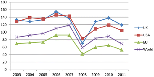
We further argue that the importance of the stock and bond markets is crucial due to their wealth effects on the real economy. The increase in the value of assets can lead to an increase in wealth of their holders and result in increased consumption and economic growth (Airaudo et al., 2011; Caporale & Soliman, 2010; Case, Quigley, & Shiller, 2012). Moreover, the wealth effects differ in countries with various weightings of the financial sector in the national economy. For instance, due to its relatively large financial sector, the wealth effects are rather more important in the British economy than many other countries (Altissimo et al., 2005). Figure 1 can provide the evidence.

Figure 1. Market capitalization relative to national income (% of GDP).

Source: World Bank’s World Development Indicators (2013).

By recognizing the interaction of financial sector (stock and bond markets) stability, wealth effects on the real economy and optimal macroeconomic policy, the objectives in this study are twofold, one is to empirically evaluate the optimal macroeconomic policy combinations and another is to analyse the symmetry (homogenous or heterogeneous) of the responses of financial markets to macroeconomic policy interactions. By so doing, we acknowledged the significance of stock and bond markets to the wealth effects on the real economy. A policy combination can only be optimal if it positively contributes to one market e.g. stock or bond, and have no adverse effects on the other and vice versa. In our study, we consider the long-term behaviour of financial markets being impacted by macroeconomic policy combinations rather than short-term effects (news). Specifically, we analyse whether both stock and bond markets move in the same or different directions in response to a particular macroeconomic policy combination.

The rationale of this paper can be drawn from a number of studies. For example, Carroll (2004) argued that wealth effects mostly persist in the medium term and also confirmed by Carroll, Otsuka, and Slacalek (2011); the financial stability is defined as the oscillation of financial asset prices and performances of financial (stock and bond) markets (Foot, 2003; Khorasgani, 2010, pp. 20–21); an increase in wealth is attributed to a rise in asset prices (see Airaudo et al., 2011; Funke et al., 2011; Malikane & Semmler, 2008); stock prices are significant indicators of financial crises (Broome & Morley, 2004).

We find that the disciplined fiscal and accommodative monetary policy stances are optimal for financial sector stability and fiscal indiscipline countered by contractionary monetary stance adversely affects financial sector stability. Financial markets (e.g. stocks and Gilts) show a short-term asymmetric response to macroeconomic policy interaction and to each other. The results generally support a number of researches in the literature (e.g. Bénassy, 2003; Benigno, Chen, Otrok, Rebucci, & Young, 2012; Khorasgani, 2010; Kontonikas & Montagnoli, 2006; Mishkin, 2011; Nakov & Thomas, 2011) and will be discussed later.

The rest of the paper is structured as follows. Section 2 provides a brief review of the literature on the subject of the study. Section 3 presents the NK-DSGE model. Section 4 presents the empirical results. Section 5 discusses and concludes this study.

2. Brief literature review

The association of the financial sector to the economy can be dated to Minsky’s (1974) famous theory of Financial Instability Hypothesis. Despite being limited to private sector debt, this theory is categorized as the pioneer in highlighting financial sector importance for the real economy, and yet financial market variables have not normally been incorporated in macroeconomic policy formulation. After Minsky, the literature has developed the debate in this field, for example, the effects of macroeconomic policies on the financial sector are reported in studies such as Bredin, Hyde, and Reilly (2005), Ardagna (2009) and Arnold and Vrugt (2010). The debate is extended to whether macroeconomic policy should consider financial market dynamics when financial stability has not been the mandate of macroeconomic policy-makers for a long time. On this issue, criticizing monetary policy stance in the real world, Mishkin (2011) argued that “although central bankers were aware that the financial sector has an important effect on economic activity, financial frictions were not an element of the pre-crisis (current financial crisis) monetary policy”. Borio (2011, p. 15) stated that “no such agreement as yet exists concerning whether, and if so, how monetary policy frameworks should be adjusted to better support financial and macroeconomic stabilities". The debate has expanded much as a result of the last financial crisis, as we can see now that the responses of stock and bond markets to monetary policy are acknowledged by the Bank of England (2011) who states that bonds and equities are inversely related to interest rates due to the high rates on which future income is discounted.

However, there is no consensus among economists on this subject in favour of the role of monetary policy in financial stability. On the contrary, Nakov and Thomas (2011) rejected monetary policy role in financial stability and argued that optimal monetary policy should only be strictly inflation targeting. Similarly, a number of studies has also denied the aggressive use of expansionary monetary policy for financial markets stability and argued that it could adversely affect the real economy (see Airaudo, Nisticò, & Zanna, 2015; Bernanke & Gertler, 2001; Di Giorgio & Nisticò, 2007). The study of Albulescu (2011), on the other hand, claimed that a monetary policy role in financial stability did not appreciate in some quarters, but it was necessary that financial stability should also be an objective of monetary policy.

With regards to macro-prudential policies, empirical evidence has also shown some disagreement. Some studies advocate that financial stability and growth can be achieved using macro-prudential policies in addition to the unconventional instrument of Asset Purchases, for example, Quantitative Easing has been used by the BoE to address some of the side effects of the financial crisis. However, Cúrdia and Woodford (2011) dismiss it and think it is not useful as it may depress the returns (yield) on financial assets. Similarly, Agénor and Pereira da Silva (2012) and Borio (2011) asserted that macro-prudential policies are insufficient for financial stability and are in favour of monetary actions. Furthermore, Svensson (2012) and Collard, Dellas, Diba, and Loisel (2012) stated that monetary policy (e.g. interest rate cut) should only be used as a last resort in financial crisis when prudential polices are inadequate. Mishkin (2011) suggested monetary policy solution on its own however can also be limited when there is a liquidity trap and this case is observed in many economies at the moment.

In terms of the functions of macro-prudential and macroeconomic policies, macro-prudential policies are considered as preventative whereas macroeconomic policies are preventative as well as reactive. This feature of monetary and fiscal policies makes them stand apart. In a recent study on the role of fiscal policy, Benigno et al. (2012) showed that fiscal policy was effective both pre- and post-Global Financial Crisis. Similarly, Mishkin (2011) claimed that the global financial crisis was so severe that it overwhelmed the ability of conventional monetary policy to counteract on its own, and advocated fiscal policy only acting as a complementary tool. In fact, the existing literature has devoted less attention to investigating the association between fiscal policy and the financial sector, compared to the role played by monetary policy (Ardagna, 2009). Blanchard et al. (2010) explained the reason behind this as firstly, in the past two decades, fiscal policy took a backseat to monetary policy because of the wide scepticism about the effects of fiscal policy on the economy, largely based on the Ricardian Equivalence¹; secondly, if monetary policy could achieve stable prices and output, there was little reason to use another instrument.

Whereas the coordination between macroeconomic policies in the literature has been widely perceived as beneficial, this may not be so practical. For instance, Niemann and Hagen (2008) noticed that independent central banks are normally reluctant to coordinate with fiscal authorities. Particularly to the UK economy, Fragetta and Kirsanova (2010) noted that fiscal and monetary policies act without effective coordination. Auerbach and Gorodnichenko (2011) also found heterogeneity in impacts of fiscal policy on different sectors of the economy. Furthermore, due to country wise heterogeneity, Baum, Poplawski-Ribeiro, and Weber (2012) called for a tailored use of fiscal policy and a country-by-country assessment of their effects. Thus, sectoral and country-wise heterogeneity of monetary and fiscal policies implies that there might be a very unique optimal policy combination in a particular financial sector context. Hence, it may not be appropriate to generalize the existing evidence of policy combinations on the real economy to the financial sector. On the top of that, the UK financial market has several unique features which make it stand apart (see Yang, Zhou, & Wang, 2009). In other words, the policy guidelines drawn on the basis of a particular sector or economy should only be applied to other sectors or economies with caution.

3. Empirical framework

In this section, we analyse the implications of optimality of policy combination for financial stability by employing the New Keynesian Dynamic Stochastic General Equilibrium (NK-DSGE) framework. The model is estimated using the Bayesian approach which has fundamental differences with the Frequentist Approach used to estimate the Vector Auto-regression (VAR) model used by Nasir et al. (2015). Our DSGE model in this paper is Stochastic, whereas in Nasir et al. (2015) was Deterministic.

DSGE modelling has become very popular in recent years. Arguing in favour of the importance and evolution of these models, Fernández-Villaverde (2009) said that the estimation of the DSGE model using combinations of rich structural models, novel solution algorithms and powerful simulation techniques have created a new discipline, which the paper labelled New Macro-econometrics. A number of recent studies have praised the DSGE framework for instance Bhattarai (2008), Gertler, Sala, and Trigari (2008), Consolo, Favero, and Paccagnini (2009), Chari (2010) and Fernández-Villaverde (2009). There are certain features of this framework. For instance, they are useful for aggregate and disaggregate level analyses which make DSGE framework useful to correspond with structural aspects of market failure (inefficiency) and distortions. DSGE is based on strong micro-foundations which overcome the Lucas critique that macroeconomic models do not capture agents’ behaviour well due to their aggregate nature. However with regards to this study, we could not find evidence of a DSGE model which has incorporated both stock and bond markets in its analysis. Furthermore, on the basis of an extensive review of the literature on the subject, we believe this study is a first attempt to derive an optimal policy combination for financial stability in a NK-DSGE framework.

Bhattarai (2008) argued that DSGE and econometric frameworks should be considered complementary techniques rather than competitive. Providing rationale for his claim, existing econometric frameworks do not focus enough on the optimization behaviour of households and firms. It is argued that this deficiency can be fulfilled using a DSGE framework. Interestingly and specifically to the UK economy, Kamber and Millard (2010) showed that the DSGE technique explained the responses of macroeconomic variables to monetary policies very well. The choice exists to use a NK-DSGE model or Real Business Cycle model. Preference for NK-DSGE over the RBC model is supported by empirical evidence, which shows that nominal rigidities (see Taylor, 1999) exist and money is non-neutral (see Christiano, Eichenbaum, & Evans, 1999) at least in the short-term characteristics which the latter can address better than the former.

In terms of data and variables in this study, we have four variables of prime interest i.e. Monetary Policy, Fiscal Policy, Stock market and sovereign bond market. We used a set of data where all observations are in monthly frequency (January 1985 to August 2008) due to the fact that the stock and bond markets exhibit quite volatile behaviour and low frequency data could ignore important aspects. Perhaps the study by Hautsch, Kyj, and Malec (2011) supported the notion of using higher possible frequency data. On the policy side, we consider using the Bank of England’s Bank Rate as the most suitable proxy for monetary policy. On this choice, one could refer to the study by Bernanke and Blinder (1992) as they argue that federal funds rates are good measures of monetary policy, i.e. the UK equivalent is the Bank Rate. The fiscal policy is proxied by Public Sector Net Cash Requirements formally known as Public Sector Borrowing Requirements as a percentage of GDP. It represents the fiscal deficit and is used as the monthly proxy for fiscal policy representing the fiscal stance. Considering the common practice in the literature on choice of proxy for fiscal policy, we could have either used debt or deficit to income (GDP) ratios, however we chose the latter, the rationale of doing so is supported by Muscatelli, Tirelli, and Trecroci (2004) as they declared a deficit as a better proxy for fiscal policy stance than debt.

The monthly averages of real Yield on UK Government bonds (Gilts) are used as a proxy for the bond market’s response. We reconstructed the raw monthly Real Government Liability Curve data from the Bank of England UK yield curve (forward curve) on 10-year UK Government bonds (Gilts) as a monthly average. We selected this data-set (following Campbell, 1995) due to the reason that it is adjusted for inflation and because the forward yield curve incorporates the expectations of significant economic agents and so also reflects the decision-making process of those agents that may manifest as forms of observable stability and instability (fluctuations). As such it reflects the confidence of market participants and investors in bonds as well as returns on investment (see David Gulley & Sultan, 2003; Nasir & Soliman, 2014). The yield on bonds is also important for the government as it represents its borrowing cost. We consider this cost to be of interest at any level rather than, following Reinhart and Rogoff (2009), an indicator that signals an ostensibly (which is now disputed, see Herndon, Ash, & Pollin, 2014) prohibitive threshold.² The stock market is proxied by monthly average prices of the FTSE-100 index. Stock market data are dividend adjusted so it incorporates the earning effects. The raw daily adjusted closing price data were converted for the FTSE 100 index to a monthly average. We selected this data-set rather than the FTSE All Share, 350 or 250 because the 100 constitutes approximately 80% of the capitalization of equity markets and contains most of the corporations in which institutional investors are empowered to trade and so is the main focus of significant trading activity. Stock-market activity is widely acknowledged to be important because it creates wealth effects (see Airaudo et al., 2015; Tsouma, 2009), and is also a potential site where adverse effects can begin or be observed (Friedman, 1988, for example, notes that a rise in stock prices may create a knock on effect to rising expected/offered returns on risky assets, whilst a rise in the volume and frequency of financial transactions creates a further transactional demand for money; see also Funke et al., 2011). Again, as with the Bond market we consider the Stock market to be of potential interest at levels below any threshold set to capture manifest instability. All data are collected from the Office of National Statistics, FTSE Group and the Bank of England.

3.1. The NK-DSGE model

The NK-DSGE model employed in this study is to some extent similar to Muscatelli et al. (2004), Airaudo et al. (2015), Giorgio and Nistico (2008), Ratto, Roeger, and Veld (2009), Zubairy (2009), Mattesini and Nisticò (2010), Kamber and Millard (2010) and Funke et al. (2011). However, as we aim to derive an optimal macroeconomic policy combination which could lead to a relatively long lasting positive impact on stock and bond markets significantly contributing to financial stability through wealth effects-real economy dynamics, the framework below is thus followed.

3.1.1. Representative household

There is a representative household with income constraint, a utility function and preferences. The Euler equation would be derived from utility function as follows:(1) $${\text{max}}_{ct,lt}U=E^0\sum _{t=0}^{\infty }{\mathit{\beta }}_{t}u(c_t,l_t)$$(1)

The objective of the household is to maximize utility (U) from a stream of consumption (c) and leisure (l), E⁰ is the expectation operator (rational expectations) based on an agent observing all current macroeconomic variables and β ∊ (0; 1) is the discount factor, while u is instantaneous utility function and c_t and l_t are levels of consumption and leisure at time t.

We have constituted the portfolio of a household with two types of assets i.e. stock(s) and government bonds (b). The wealth of the household is generated by two sources which are financial wealth (A) which consist of income from financial assets (stock and bonds) and non-financial wealth (H) which is labour income. Therefore, the total financial wealth would be as follows:(2) $$A=\sum _{i=1}^{\infty }s+b$$(2)

The intertemporal consumption of the household depends on wealth, hence,(3) $$C=mp{c}_w[A+H(Y)]\approx mp{c}_{w}A+mp{c}_{Y}Y$$(3)

where C is the consumption, A is financial wealth and H represents human wealth (the present value of expected labour income (net of taxes) Y. The (mpc) is the proportionality coefficient which measures the marginal propensity to consume (MPC) out of financial wealth and income, respectively. Transforming Equation (3) into an elasticity form yields the following:(4) $$\frac{\mathrm{\Delta }c}{c}=\underset{e_w}{\underbrace{\left[mp{c}_w\frac{A}{c}\right]}\frac{\mathrm{\Delta }A}{A}}+\underset{1-e_w}{\underbrace{[mp{c}_Y\frac{Y}{c}}}]\frac{\mathrm{\Delta }Y}{Y}=\underset{e_{wj}}{\underbrace{\sum mp{c}_w\frac{A_j}{C}\frac{\mathrm{\Delta }{A}_j}{A_j}}}+[mp{c}_Y\frac{Y}{C}]\frac{\mathrm{\Delta }Y}{Y}$$(4)

Equation (4) shows that the wealth elasticity of consumption (e_w) depends on the $mp{c}_w$ as well as wealth consumption ratio of each component j.

3.1.2. Firms

We have a representative firm which operates under monopolistic competition. The objective of the firm is to maximize the cost constrained profit. The production technology (Cobb-Douglas) is as follows:(5) $$Y_t=z_{t}f(k_t,n_t)$$(5)

While $Y_t$ is the unit of goods produced, k_t and n_t symbolize quantities of physical capital and labour allocated to the production process and $z_t$ denotes a random disturbance to productivity (technology shock). However, the production sector is composed of wholesale and retail sectors. The behaviour of firms in the wholesale sector would be:

(6) $$Y_t^w=z_{t}f(k_{t-1},n_t)$$(6)

K_t is the end of period capital stock. To incorporate monopolistic competition, the production function for the wholesale sector (6) would be converted into differentiated goods in (7) at the cost $c{Y}_t^W$ as retail output below:

(7) $$Y_t=\left(1-C\right)Y_t^w$$(7)

Time is divided between labour (n) and leisure (l), hence each unit of time would be divided as follows:

(8) $$1=n_t+l_t$$(8)

Each unit of the output produced in time t is either consumed (c) or invested in stock of capital (i), hence:

(9) $$Y_t=c_t+i_t$$(9)

Stock of capital evolves according to law of motion of capital given by,

(10) $$K_{t+1}=i_t+(1-\mathit{\delta })k_t$$(10)

Here δ denotes the depreciation rate of capital. There are two explicit trades-offs in the above scenario i.e. labour/leisure and saving/investment trades-offs. However, we put no stress on their details at this stage. The stochastic process of productivity would be:

(11) $$z_t=\mathit{\rho }{z}_t-1+set$$(11)

where(11) $$e{t}^{\sim }N(0,{\mathit{\sigma }}^2)$$(11)

3.1.3. Monetary authority

We have a central bank which controls money supply, and the monetary authority follows a Taylor rule and would be incorporated in the model following Clarida, Gali, and Gertler (2000) as:(12) $$r_t=\mathit{\rho }r{r}_{t-1}+\mathit{\rho }\mathit{\pi }{\mathit{\pi }}_t+\mathit{\rho }g{g}_t+\mathit{\rho }o{o}_t+\mathit{ϵ}{r}_t^{\sim }N(0;\mathit{\sigma }2r)$$(12)

where r_t is the rate of interest, ${\mathit{\pi }}_t$ is gross inflation rate, $g_t$ represents gross output growth rate, $o_t$ is the output gap and ρ is the parameter denoting elasticity and response of monetary authority to deviation of inflation and output from their steady states.

3.1.4. Fiscal authority

To represent the government or fiscal authority which levies taxes to fund its spending over a variety of goods, we use a backward looking fiscal rule as suggested by Muscatelli et al. (2004). The reason for this is that it shows a response of fiscal policy to deviation of macroeconomic variables. However, it is interesting in our case as we are extending it to the financial sector and therefore it will capture the response of fiscal authority to dynamics in the financial market. The exogenous process is as follows:

(13) $$G_t-G_{sst}=\mathit{\rho }G*(G_{t-1}-G_{sst-1})+\mathit{ϵ}G$$(13)

where $G_t$ is fiscal spending, $G_{sst}$ is the fiscal stance in steady state and ρG fiscal spending parameter. The balanced budget constraint adopts the following form:

(14) $$G_t=h\ast WP\ast tax$$(14)

where h is labour hours, WP is the wage rate and tax is the government levy on labour income.

3.1.5. Investment cost (Smets–Wouters)

We also introduce an investment cost in our model following Smets and Wouters (2007) which disappears in the long-run. The model adopts the following form:

(15) $$K_t=(1-\mathit{\delta })K_{t-1}+(1-S(X_t))I_t$$(15)

whereas K is the capital stock, δ is depreciation rate, S is the investment cost, I is the output,

$S^1,S^{{}^{\prime \prime }}\ge 0;S(1+g)=S^{{}^{\prime }}(1+g)=0$and $X_t=\frac{l_t}{l_{t-1}}$

The capital producing firm at time t coverts I_t of output into (1 – S (X_t)) I_t of new capital sold at a real price Qt, and the expected discounted profits are maximized with respect to {I_t}$$E_t\sum _{k=0}^{\infty }{D}_t,t+k[Q_{t+k}\left(1-S\left(\frac{l_{t+k}}{l_{t+k-1}}\right)\right)l_{t+k}-l_{t+k}$$

$D_t,t+k={\mathit{\beta }}^k(\frac{\mathrm{\Lambda }c,t+1}{\mathrm{\Lambda }c,t}$) is the real stochastic discount rate over the interval [$t,t+k$]. It takes us to first-order condition,

$$Q_t(1-S(X_t)-X_t{S}^{{}^{\prime }}(X_t))+E_t[D_{t,t+1}{Q}_{t+1}{S}^{{}^{\prime }}(X_{t+1})\frac{l_{t+1}^2}{l_t^2}]=1$$

In addition the capital demand by firm must satisfy the following condition

$$R_t=\frac{E_t[1-\mathit{\alpha })\frac{P_{t+1}^w}{P_t}\frac{Y_{t+1}}{K_t}+(1-\mathit{\delta })Q_{t+1}]}{Q_t}$$

The right-hand side of the above equation indicates the gross return on holding one unit of capital from period t to t + 1. It is also considered as gross return from bond holding or opportunity cost of capital (R_t). In the long run, these investment costs fade away hence S = 0 and Qt = 1 and we arrive at the functional form:

$$S(X)={\mathrm{\Phi }}_x{(X_t-(1+g))}^2$$

Where g represents the balanced growth path and it is worth mentioning that along a balanced growth path X_t = 1 + g and investment cost fades away. Levine (2012) declared it as a convenient feature because the steady state is unaltered by investment cost.

3.1.6. Price stickiness

We introduce price stickiness in the form of staggered price setting in retail sector with Dixit and Stiglitz (1977) monopolistic competition which uses homogenous wholesale goods to produce a basket of differentiated goods for consumption (Levine, Pearlman, Perendia, & Yang, 2012) as:

(16) $$C_t={(\underset{0}{\overset{1}{\int }}{c}_t{(m)}^{\frac{\mathit{\zeta }-1}{\mathit{\zeta }}}dm)}^{\frac{\mathit{\zeta }}{\mathit{\zeta }-1}}$$(16)

Where the consumer chooses consumption goods C_t(m) at a price P_t (m) to maximize (1) and total expenditure becomes $\underset{0}{\overset{1}{\int }}{P}_t$ (m) $C_t$(m) dm and ζ is elasticity of substitution. It leads to a set of consumption demand equations for each differentiated good m with price P_t (m). $P_t$is the aggregate price index given as:

$$P_t={[\underset{0}{\overset{1}{\int }}{P}_t{(m)}^{1-\mathit{\zeta }}dm]}^{\frac{1}{1-\mathit{\zeta }}}$$

Both C_t and P_t are Dixit–Stiglitz aggregates as detailed in Dixit and Stiglitz (1977). The demands for investment and government services remain the same, therefore in aggregate:

$$Y_t(m)={(\frac{P_{t(m)}}{P_t})}^{-\mathit{\zeta }}{Y}_t$$

To incorporate price stickiness here, we follow Calvo (1983) and assume that there is a probability of 1 – ζ at each period that the price of each retail good (m) is set optimally to $P_t^0$(m). In case the price is not re-optimized then it remains fixed, hence $\frac{1}{1-\mathit{\zeta }}$ can be interpreted as the average time during which prices are unchanged (sticky). The objective of each retail firm (m) at time t is to choose $P_t^0(m)$ at given real marginal cost $M{C}_t$ to maximize the discounted profits given as:

$$E_t\sum _{k=0}^{\infty }{\mathit{\zeta }}^k{D}_{t,t+k}{Y}_{t+k}(m)[P_t^0(m)-P_{t+k}M{C}_{t+k}]$$

where D_t,t+k is the nominal stochastic discount factor over the interval [t, t + k], the marginal cost MC_t = $P_t^w$ / P_t is no longer fixed and the solution adopts the following form

$$E_t\sum _{k=0}^{\infty }{\mathit{\zeta }}^k{D}_{t,t+k}{Y}_{t+k}(m)[P_t^0(m)-\frac{1}{(1-\frac{1}{\mathit{\zeta }})}{P}_{t+k}M{C}_{t+k}]=0$$

The price index in evaluated by the law of large numbers as

$$P_{t+1}^{1-\mathit{\zeta }}=\mathit{\zeta }{P}_t^{1-\mathit{\zeta }}+(1-\mathit{\zeta }){(P_{t+1}^0)}^{1-\mathit{\zeta }}$$

As the last step, the price dispersion ${\mathrm{\Delta }}_t$ reduces the output and is presented as below

$$Y_t^w=\frac{{(A_t{h}_t)}^{\mathit{\alpha }}{K}_{t-1}^{1-\mathit{\alpha }}}{{\mathrm{\Delta }}_t}$$

where ${\mathrm{\Delta }}_t\equiv \frac{1}{n}\sum _{j-1}^n{(P_t(j)/P_t)}^{-\mathit{\zeta }}=\mathit{\zeta }{\mathrm{\Pi }}_t^{\mathit{\zeta }}{\mathrm{\Delta }}_{t-1}+(1-\mathit{\zeta }){(\frac{j_t}{H_t})}^{-\mathit{\zeta }}$

Nevertheless, the price dispersion ${\mathrm{\Delta }}_t$ here is of second order, therefore for a first-order approximation we would have ∆ = 1 as value of its steady state.

3.1.7. Financial sector

The core part of our model is the incorporation of a particular aspect of financial markets i.e. stock and bond markets into the analysis. Following David, DeJong, and Dave (2007), multi-asset portfolio would be represented which includes risk-free (government bond) and risky (stock) assets as:(17) $$C_t+P_t^e\left(S_t^e+S_{t-1}^e\right)+P_t^f\ast S_t^f=d_t\ast S_{t-1}^e+S_{t-1}^f+q_t$$(17)

In the above scenario $P_t^e$ denotes the price of the risky asset, $S_t^e$ represents the number of shares held in the asset during period t − 1, d_t represents dividend payment, q_t is exogenous stochastic endowment and $P_t^f$ and $S_t^f$ are analogous for the risk-free asset. The risk-free asset pays one unit of the consumption good at time t if held at time t − 1 (hence the loading factor of 1 associated with $S_{t-1}^f$on the right-hand side of the budget constraint).

3.2. Bayesian estimation and Bayes’ theorem

We estimate our NK-DSGE model using Bayesian estimation technique. This approach has significant advantages over others including full information approach which fits the model to all variations and data and not only to the impact of policy (Zubairy, 2009). In an earlier study, arguing in favour of Bayesian estimation, Milani and Poirier (2007) stated that the micro-foundation and the Bayesian approach have made the DSGE model to stand apart from the models built on dogmatic prior for structural parameters. Similarly, study by Merola (2009) showed that for large samples, maximum likelihood asymptotically converges to Bayesian estimation. A notable advantage of Bayesian approach is the ability to provide a framework for evaluating even the most fundamentally misspecified models.

Bayesian estimation is based on Bay’s theorem which can be represented as follows:

Assume that θ is the parameter of interest then p(θ) represents the prior density of the parameter vector θ,

$$p(\mathit{\theta }|yT)=\frac{L(yT|\mathit{\theta })p(\mathit{\theta })}{{\int }_{\mathrm{\Theta }}^{}L(yT|\mathit{\theta })p(\mathit{\theta })d\mathit{\theta }}\propto L(yT|\mathit{\theta })p(\mathit{\theta })$$

L(y |θ) is the likelihood of the sample y with T observations where ${\int }_{\mathrm{\Theta }}^{}$L(y |θ) P (θ) d (θ) is the marginal density of the sample and P (θ|y) is posterior density.

In essence, we start from prior belief on θ, and modify our belief or revise probabilities when we observe data. Application of this approach and the above-mentioned advantages would also give us some insight into the validity and sturdiness of our optimal policy combination in the context of alternative empirical estimation approaches.

3.3. Markov chain Monte Carlo (MCMC)–Metropolis Hasting (MH) algorithm

To acquire random draws from the posterior distribution, we apply the Markov Chain Monte Carlo–Metropolis Hasting (MCMC–MH) algorithm. There are two famous algorithms i.e. Metropolis Hastings and Gibbs Sampling. However, we employ the first one which is also the first MCMC method employed in the literature with several advantages. Description of them would be beyond the scope of this study. However, the main idea of using Metropolis Hastings algorithm is that it samples from the region with highest probability but also visits wide parameter space. The next value of the MCMC chain is generated from proposal density and acceptance or rejection depends on value of the target density at the candidate point relative to the target density at the current point (Canova, 2007).

Hereafter we move towards estimation and policy simulation of our model. To start with, we incorporate equity and bond markets into our analysis to derive optimal policy combination.

4. Empirical analysis and findings

There is a growing strand of literature on the incorporation of financial markets in DSGE models. Prominently, the remarkable milestone was laid by Nistico (2005) followed by Airaudo et al. (2015), Giorgio and Nistico (2008) and most recently Funke et al. (2011). This study similarly incorporates stock and bond markets into the NK-DSGE framework. There are five exogenous variables i.e. fiscal policy (G) monetary policy (M), technology (A), bond market (B) and stock market (S) which are given one standard deviation shock and the impact analysed on stock and bond markets.

Dynare software package version (4.3) in Matlab is used. The monthly observations of stock market (FTSE-100) and Bond market (10-year Gilts real yield) after taking the natural log into the NK-DSGE model from January 1985 to August 2008 (N = 285). The choice of this time period for analysis is made to avoid the massive fluctuation of financial markets during the global financial crisis from 2008. To deal with the issues of non-linearity in the data, we use Kalman Filter and diffuse filter option in Dynare. As mentioned earlier, we use Bayesian approach for estimation which is a full information hybrid approach which considers the prior information and deals with the misspecification of models. We also use Monte-Carlo-based optimization routine algorithm to obtain draws of posterior distribution which is an evolutionary algorithm to initialize the Metropolis Hastings (MH) and to define the jumping distribution, particularly when it is hard to obtain it with standard (Newton like) optimization routines. As an initial burn-in period, we discard 20% of our initially generated parameter vectors to remove any dependence of chain from its starting value. We also tune acceptance rate scale for jumping distribution in Metropolis Hastings to 0.40 allowing good acceptance rate (20–40%) for adjustment of covariance matrix. Figures 2 and 3 represent the historical and smooth values of our observable variables (stock and bond markets). The vertical axis (Y) represents the natural log value of stock market and real yield on 10 years of Gilts, respectively, while horizontal axis (x) depicts the observation count.

Figure 2. Historical log values of stock market (FTSE-100).

Source: Author’s calculation using Matlab (Dynare).

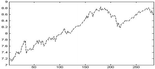
Figure 3. Historical and smoothed values of bond yield (10 year Gilts).

Source: Authors calculations using Matlab (Dynare).

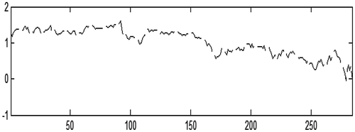
It is evident from Figures (2 and 3) that there have been non-linear moments in observable variables (stock and bond markets), although the bond market shows less volatility than the stock market. However, the aforementioned series of measures and methodological arrangements (Kalman Filter, Transformation) would overcome issues of non-linearity in the data, particularly using the Bayesian approach.

The estimation as well as simulation of the model is carried out and the findings are presented and discussed here whereas additional details of model estimations are attached as Appendix A. We start with the variance decomposition analysis as shown in Table 1. A one standard deviation shock given to the exogenous variables showed that technological shock contributed to 12.72% variation in stock and 6.38% variation in bond market. The monetary policy shock was the largest, while fiscal policy made the smallest contribution to variation in stock as well as bond market. The variation in stock and bond to a considerable extent (33.13% and 0.13%) was due to the shock emerging from the stock market. However, the shock from the bond market did not contribute much to variation in the stock market.

The conditional variance decomposition by narrowing the analysis to various periods shows that fiscal policy and financial market shocks started to fade out after a while. However, the comparative impact of monetary policy shock and to some extent technology shock increases overtime. This might be associated with the long-term impact of technological advances and money supply effects on profitability of firms which could positively be reflected in stock prices. However, we will not go further into the time variant aspect of macroeconomic policy and technological advances as it is beyond the scope of our study, hence we leave this interesting notion for future research.

To reflect on the dynamics of exogenous and observable variable (stock market) over the complete horizon of the study, we have presented the smoothed shocks to exogenous variables and responses of stock and bond markets in Appendix A. The results of policy (stochastic) simulations are presented here. An Impulse Response Function (IRF) analysis is performed in addition to the policy (stochastic) simulation. One standard deviation shock to exogenous variables including stock as well as bond markets and their responses in the following 20 periods (months) are presented in Figures (4–8).

Figure 4. Impulse response function analysis.

Source: Authors calculations using Matlab (Dynare).

Figure 5. Impulse response function analysis.

Source: Authors calculations using Matlab (Dynare).

Figure 6. Impulse response function analysis.

Source: Authors calculations using Matlab (Dynare).

Figure 7. Impulse response function analysis.

Source: Authors calculations using Matlab (Dynare).

Figure 8. Impulse response function analysis.

Source: Authors calculations using Matlab (Dynare).

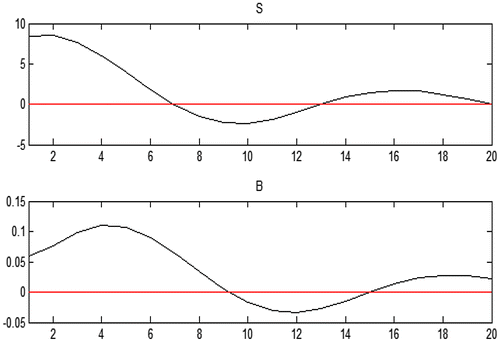
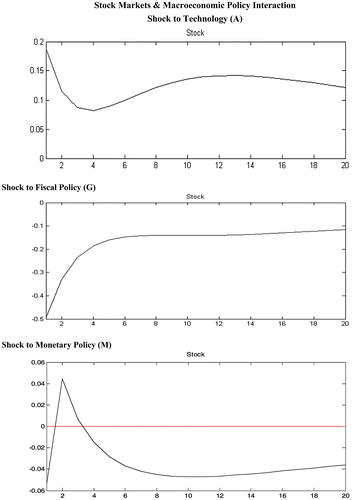
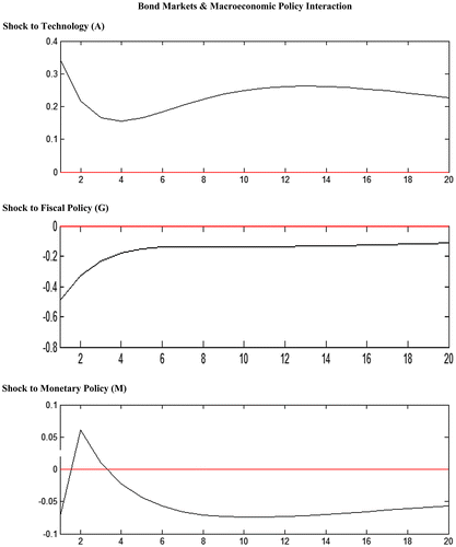
The simulation results were in line with the estimation outcome as we can see in the following Figure (4), a positive (one standard deviation) shock receives a positive response from the stock market indicating the increase in profitability of production sectors in response to technological advances. On the other hand, the bond yield initially surged before showing a slight decrease, which also indicates positive effects of technological improvements on bond markets. Hence, we could argue that structural and technological improvements in the economy are also beneficial for the financial sector. This finding is important with regard to Greenwood and Jovanovic (1999) and Bart and Jovanovic (2001) celebrated work on stock market and technology shock in which they argued that as the new technology destroys the old technology it has held the stock market performance back for some period. Our findings here extend the insight given by showing that in long term there are net gains for the stock market as well as for the bond market. Hence, the idea of constructive destruction is more constructive for the financial sector in the big picture

4.1. Technology shocks to stock and bond

As the main theme of our study is macroeconomic policy combination effects, first we present the responses of the financial sector and monetary policy to an exogenous fiscal policy (Government Spending) shock. The results are shown in Figure (5).

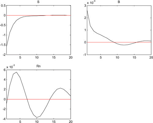
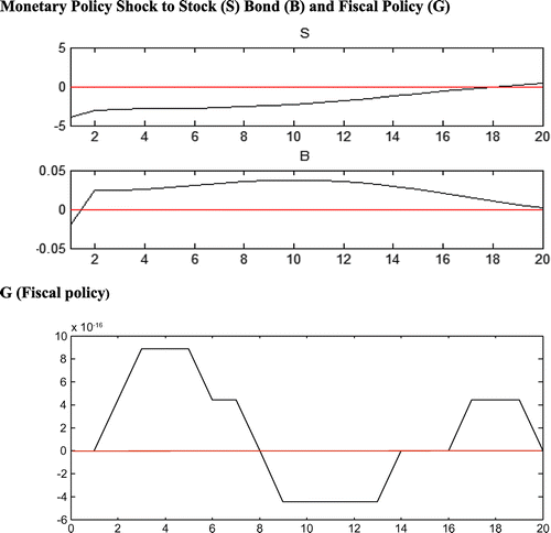
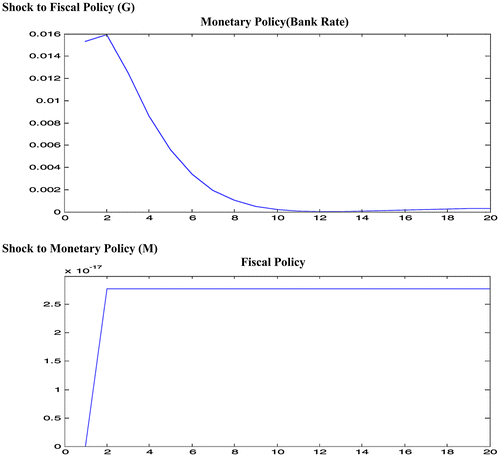
A positive (expansionary) fiscal policy shock results in an immediate decrease in stock prices which recover fully in about 10 periods. Moreover, bond yield increased implying that the prices of Gilts also decreased. In the context of policy interaction, the bank rates (Rn) used as the monetary policy instrument also increases in response to fiscal policy shock, which implies that fiscal expansion leads monetary policy to adopt a contractionary stance. It also shows that an expansionary or undisciplined fiscal policy adversely affects the financial sector. In analysing the impact of monetary stance, a contractionary monetary policy or increase in bank rate (Rn) leads to a drop in stock prices, which persists almost for 18 periods indicating the sharpness of the impact. On the other hand, the same policy shock leads to a small initial decrease which turns into a persistent increase in bond yield (fall in prices) implying that the bond market responds negatively to contractionary monetary policy. The initial increase in bond prices (decrease in yield) might be due to portfolio adjustment by households as a consequence of the policy impact.

The response of yield changed into positive in the first period (month) and returned to equilibrium nearly 20 periods later. However, on the whole, the bond market shows a negative response to monetary contraction as the yield increases showing a negative response from prices of bonds.

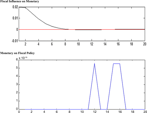
Interestingly, fiscal policy shows a very mild positive response as the value of deficit/surplus on the Y axis was quite modest $({10}^{-15})$. This seems to suggest that monetary contraction could not move fiscal authority towards a contractionary policy stance. In the context of optimal policy combination and interactions of policies, it seems to be an important finding as it seems to show that contractionary monetary policy may not bring fiscal discipline, yet it could adversely affect the stock and bond markets.

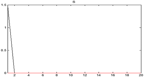
In order to analyse the interdependence between both bond and stock markets we treat them exogenously, and we find that a one standard deviation shock to bonds yield results in a sharp surge of stock market prices which return to equilibrium in only 2 periods (months). It is also an interesting finding as it implies that the increase in yield or fall in bond prices leads to an increase in stock market prices for the short term only. It is an indication of short-term asymmetry in the movements of both markets, perhaps due to portfolio adjustment, news effects and profit taking in the short term by market participants. However, the shock quickly fades away and market adjustments take place.

Similarly, a positive (one standard deviation) shock from the stock market leads to a very small increase in yield in bonds showing a negative response from the bond market which rapidly fades away. However, the bond market returns to equilibrium quite quickly showing a similar response to that from the stock market suggesting that the bond market also has a short-term asymmetric response. Therefore, this might suggest that in the long term, we might see a symmetric (homogenous) behaviour in the two markets.

To sum up, we jointly considered monetary and fiscal policies effects and found that a technological shock receives positive response from the financial sector (stock and bond) policy change. In the context of macroeconomic policies, an expansionary fiscal policy shock leads to a decrease in stock prices whereas gilt yield and bank rates increase. On one hand this implies negative responses from both markets as prices of financial assets fell, compelling the monetary authority to adopt a contractionary and conflicting policy stance. On the other hand, a positive one standard deviation shock to bank rates (monetary contraction) leads to falling stock prices after a slight initial increase. The bond yield also increases implying an overall negative response from both markets to monetary contraction. With regards to fiscal policy response we could see only a slight expansionary response implying that fiscal policy stance may not be influenced by monetary policy in any significant way. The stock and bond markets show some short-term asymmetry in their relationships as the positive response from stocks leads to a fall in bond prices whereas an increase in bond yield (fall in bond prices) leads to increases in stock prices. This asymmetry however, seems to be short term and fades away quickly. In order to test the robustness of the model we performed a sensitivity analysis by omitting the stock and bond markets alternatively and limiting our analysis of policy interaction to a single market i.e. either stock or bond markets. The results are attached as Appendix B and Figures (8 and 9). It shows that analysis of financial markets in isolation has similar results. Concomitantly, there were no changes in the derived which suggests optimal policy combination for financial stability and sensitivity analysis supporting the findings of the NK-DSGE model on the whole.

5. Conclusions

This study derived the optimal macroeconomic policy combination for financial stability in the context of the UK. The results show that technology shock results in overall positive response from the financial sector. With regards to macroeconomic policies, an expansionary fiscal policy leads to decrease in stock and bond prices but increase in bank rates. The implications are that the negative responses from both markets compel monetary authority to adopt a contractionary and a conflicting policy stance relative to fiscal authority position. On the other hand, contractionary monetary policy resulting in falling stock and bond prices imply an overall negative response from both markets to monetary contraction. There was a short-term asymmetry in responses of stock and bond markets to monetary policy interaction. However, both markets show a homogenous response in the long term, which is a vital finding indicating stability in the stock market necessitating stability in the bond market as well. The short-term asymmetry could be associated with portfolio adjustments and selling of financial assets for quick profits. Fiscal policy shows a mild expansionary response to monetary policy change implying that fiscal policy stance may not be significantly influenced by monetary policy. To each other, stock and bond markets show very short-term negative associations as the positive response from stock markets lead to a fall in bond prices whereas an increase in bond yield (fall in bond prices) leads to increase in stock prices, which is intuitive in the light of portfolio adjustment (between stock and bond) and risks premium theory. Nevertheless, this asymmetry of stock and bond markets is short term (2-month periods) and in the long term both markets show co-movements and homogenous positive responses to our optimal policy combination.

The results also suggest that a policy conflict may hamper the financial sector and non-coordination (Nash) between the two macroeconomic authorities is not beneficial since the monetary contraction did not induce fiscal discipline. On the other hand, the fiscal policy expansion leads monetary policy to a conflicting contractionary stance which adversely affects the financial sector. It also highlights the importance of fiscal policy coordination for financial sector stability, which could be considered as an extension of the FTPL theory. With regards to the optimal macroeconomic policy combination, we can conclude that this consists of disciplined fiscal and accommodating monetary policies as optimal for financial stability in the long term. Our results seem rejecting the idea that the monetary policy should only focus on price stability and ignore cooperation with fiscal authority for output growth, as such a stance would also adversely affect financial sector stability. In optimal policy context, an expansionary monetary policy with fiscal discipline (contraction) brings the best outcome for stock and bond markets. Most importantly, the results show that the fiscal and monetary policies also influence each other, as fiscal expansion leads to monetary contraction whereas monetary contractions leads to growth in deficits. Therefore, we can conclude that there is significant scope for macroeconomic policy co-ordinations which perhaps is also vital for financial sector stability.

Additional information

Funding

Funding. The authors received no direct funding for this research.

Notes on contributors

Muhammad Ali Nasir

Muhammad Ali Nasir is a senior lecturer in Leeds Beckett University, UK. His main areas of research interest are macroeconomics, financial economics, labour markets, international trade and macroeconomic modelling. Nasir also has a great interest in history of economic thought, European integration and more recently European financial crises, with which the article was inspired from. He is the corresponding author of this paper.

Milton Yago

Alaa M. Soliman is a senior lecturer in Leeds Beckett University, UK. His main areas of research interest are macroeconomics, financial economics, econometrics and macroeconomic modelling.

Alaa M. Soliman

Milton Yago is a senior lecturer in Leeds Beckett University, UK. His main areas of research interest are macroeconomics, international trade, microeconomics and DSGE modelling.

Junjie Wu

Junjie Wu is a senior lecturer in Leeds Beckett University, UK. Her wide research interests across accounting, finance and economics. She is particularly interested in SME and CSR related issues.

Notes

1. There are no permanent effects of fiscal policy as government spending at present is offset by future tax hike, hence there would be no long term real impact on the economy.

2. Please refer to Nasir et al. (2015) for a detailed discussion on using financial variables at aggregate level and rate rather thresholds to proxy level of financial stability.

Appendix A

Table 1. Variance decomposition analysis of stock and bond markets

Variance decomposition (%)	epsA^*	epsG^**	epsM^***	epsS^****	epsB^*****
Stock	12.72	0.16	53.87	33.13	0.13
Bond	6.38	0.00	72.68	20.94	0.00
Conditional variance decomposition (%)
Periods	1
	epsA	epsG	epsM	epsS	epsB
Stock	21.77	0.79	4.2	72.35	0.89
Bond	1.84	0.00	97.46	0.69	0.00
Periods	4
	epsA	epsG	epsM	epsS	epsB
Stock	32.85	0.50	21.26	44.99	0.40
Bond	5.05	0.00	77.52	17.43	0.00
Periods	10
	epsA	epsG	epsM	epsS	epsB
Stock	15.05	0.20	49.81	34.77	0.16
Bond	6.70	0.00	73.75	19.55	0.00
Periods	100
	epsA	epsG	epsM	epsS	epsB
Stock	12.72	0.16	53.87	33.13	0.13
Bond	6.38	0.00	72.68	20.94	0.00

^* Technology shock.

^** Fiscal.

^*** Monetary.

^**** Stock.

^***** Bond shocks.

Source: Author’s calculations using Matlab.

Table 2. Matrix of coorelation-simulated variables

Variables	Stock	Bond (Yield)	Monetary (BR)	Fiscal (PSNBR/GDP)
Stock	1	0.4462	0.8484	−0.0401
Bond (Yield)	0.4462	1	0.7597	0.0032
Monetary (BR)	0.8484	0.7597	1	0.0002
Fiscal (PSNBR/GDP)	−0.0401	0.0032	0.0002	1

Table 3. Auto-correlation of simulated variables

Variable	1	2	3	4	5
Stock	0.8109	0.4994	0.1391	−0.1948	−0.441
Bond	0.816	0.5451	0.2141	−0.1087	−0.362
Monetary	0.7674	0.4222	0.0458	−0.2837	−0.5087
Fiscal	0.5573	0.3105	0.1731	0.0964	0.0537

Table 4. Theoratical momnets of simulated variables

Variable	Mean	Std. Dev	Variance
Stock	4.6363	47.4902	2255.3199
Bond	−0.3043	0.9946	0.9893
Monetary (Rn)	1.0131	13.5462	183.4989
Fiscal (G)	3.1369	3.7644	14.1707

Table 5. Matrix of covariance of exogenous variables

Variables	epsA	epsG	epsRn	epsS	epsB
epsA	1.012992	0	0	0	0
epsG	0	0.99286	0	0	0
epsRn	0	0	22.08881	0	0
epsS	0	0	0	4.367687	0
epsB	0	0	0	0	2.860742

Table 6. Results from posterior maximization parameters

prior	mean	mode	s.d.	t-stat	prior	pstdev
rhoA	0.500	0.830	0.003	248.189	beta	0.200
rhoG	0.500	0.557	0.006	98.603	beta	0.200
phiX	2.000	3.255	0.010	322.992	norm	1.500
sigma_c	1.500	1.328	0.004	369.145	norm	0.375
varrho	0.500	0.091	0.002	42.997	beta	0.200
xi	0.500	0.888	0.000	2050.296	beta	0.100
alp	0.700	0.536	0.001	733.325	beta	0.050
alpha_pie	1.500	0.889	0.011	78.011	norm	0.250
alpha_r	0.750	0.548	0.002	301.430	beta	0.100
epsilon	0.500	0.020	0.002	11.111	beta	0.200
Standard deviation of shocks
prior	mean	mode	s.d.	t-stat	prior	pstdev
epsA	0.100	1.007	0.029	35.129	invg	2.000
epsG	0.500	0.996	0.018	56.802	invg	2.000
epsRn	0.100	4.700	0.046	101.916	invg	2.000
epsS	0.100	2.090	0.046	45.012	invg	2.000
epsB	0.100	1.691	0.038	44.369	invg	2.000

Note: Log data density [Laplace approximation] is −2,809.534823.

Table 7. Policy and transition functions

	Stock	Bond	Monetary (Rn)	Fiscal (G)
Constant	4.63632	−0.304326	1.013069	3.137
K (−1)	0.344092	−0.001805	0.042118	0.000
I (−1)	0.341154	−0.009625	0.134008	0.000
A (−1)	2.932403	0.020595	0.167531	0.000
G (−1)	−0.284339	0.000467	−0.000176	0.557
Rn (−1)	1.421675	0.049022	0.719129	0.000
PIE (−1)	1.699488	−0.004016	0.371119	0.000
B (−1)	7.283923	−0.017212	1.590597	0.000
epsA	8.295611	0.058263	0.473936	0.000
epsG	−1.60061	0.002629	−0.000992	3.137
epsRn	0.780035	0.090683	1.330278	0.000
epsS	−7.284	0.017	−1.591	0.000
epsB	1.000	0.000	0.000	0.000

Appendix B

Stock Markets & Macroeconomic Policy Interaction

Figure 9 Impulse response function analysis. Source: Authors calculations using Matlab.

Figure 10 Impulse response function analysis. Source: Authors calculations using Matlab.

Shock to Technology (A)

Shock to Fiscal Policy (G)

Shock to Monetary Policy (M)

Shock to Fiscal Policy (G)

Monetary Policy(Bank Rate)

Shock to Monetary Policy (M)

Fiscal Policy

Bond Markets & Macroeconomic Policy Interaction

Shock to Technology (A)

Shock to Fiscal Policy (G)

Shock to Monetary Policy (M)

Fiscal Influence on Monetary

Monetary on Fiscal Policy

References

- Agénor, P. R., & Pereira da Silva, L. A. (2012). Macroeconomic stability, financial stability, and monetary policy rules. International Finance, 15, 205–224.10.1111/j.1468-2362.2012.01302.x
- Airaudo, M., Nisticò, S., & Zanna, L. F. (2015). Learning, monetary policy, and asset prices. Journal of Money, Credit and Banking, 47, 1273–1307.10.1111/jmcb.2015.47.issue-7
- Airaudo, M., Cardani, R., & Lansing, K. J. (2011). Monetary policy and asset prices with belief-driven fluctuations and news shocks. Philadelphia, PA: LeBow College of Business, Drexel University. Retrieved from http://www.be.wvu.edu/econ_seminar/documents/11-12/airaudo.pdf
- Albulescu, C. T. (2011). Macro-financial risks and central banks: What changes has the crisis triggered? Timisoara Journal of Economics, 4, 135–142.
- Altissimo, F., Georgiou, E., Sastre, M., Valderrama, M. T., Stocker, G. S. M., Weth, M., Whelan, K., & William, A. (2005). Wealth and assets price effects on economic activity (Occasional Paper Series No 29). European Central Bank. Retrieved from http://papers.ssrn.com/sol3/papers.cfm?abstract_id=752089
- Ardagna, S. (2009). Financial markets’ behavior around episodes of large changes in the fiscal stance. European Economic Review, 53, 37–55.10.1016/j.euroecorev.2008.07.003
- Arnold, I. J. M., & Vrugt, E. B. (2010). Treasury bond volatility and uncertainty about monetary policy. Financial Review, 45, 707–728.10.1111/(ISSN)1540-6288
- Auerbach, A. J., & Gorodnichenko, Y. (2011). Measuring the output responses to fiscal policy. Berkeley: Department of Economics, University of California. Retrieved from https://www.aeaweb.org/articles.php?doi=10.1257/pol.4.2.1
- Bank of England. (1997). Monetary policy framework. Author. Retrieved from http://www.bankofengland.co.uk/monetarypolicy/framework.htm
- Bank of England. (2011). The transmission mechanism of monetary policy. The Monetary Policy Committee Bank of England. Retrieved from www.bankofengland.co.uk
- Bart, H. & Jovanovic, B. (2001). The information-technology revolution and the stock market: Evidence. American Economic Review, 91, 1203–1220.
- Baum, A., Poplawski-Ribeiro, M., & Weber, A. (2012). Fiscal multipliers and the state of the economy ( WP/12/286). Washington, DC: International Monetary Fund.
- Bénassy, J. P. (2003). Fiscal policy and optimal monetary rules in a non-Ricardian economy. Review of Economic Dynamics, 6, 498–512.10.1016/S1094-2025(03)00017-6
- Benigno, G., Chen, H., Otrok, C., Rebucci, A., & Young, E.R. (2012). Optimal policy for macro-financial stability ( Working Paper 2012-041A). Research Division Federal Reserve Bank of St. Louis.
- Bernanke, B. S., & Blinder, A. S. (1992). The federal funds rate and the channels of monetary transmission. The American Economic Review, 82, 901–921.
- Bernanke, B. S., & Gertler, M. (2001). Should central banks respond to movements in asset prices? American Economic Review, 91, 253–257.10.1257/aer.91.2.253
- Bhattarai, K. (2008). Econometric and stochastic general equilibrium models for evaluation of economic policies ( Working Paper). Hull University Business School. Retrieved from http://www.hull.ac.uk/php/ecskrb/Stochastic_GE_IJTGM%204(2)%20Paper%207.pdf
- Blanchard, O., Dell’Ariccia, G., & Mauro, P. (2010). Rethinking macroeconomic policy (IMF staff Position Note, SPN/10/03).
- Borio, C. (2011). Re-discovering the macroeconomic roots of financial stability policy: Journey, challenges and a way forward (BIS Working Papers No 354).
- Bredin, D., Hyde, S., & Reilly, G. O. (2005). UK stock returns & the impact of domestic monetary policy shocks (Working Paper). Department of Banking & Finance, Graduate School of Business, University College Dublin. Retrieved from http://www.ucd.ie/t4cms/wp0604-1.pdf
- Broome, S., & Morley, B. (2004). Stock prices as a leading indicator of the East Asian financial crisis. Journal of Asian Economics, 15, 189–197.10.1016/j.asieco.2003.12.008
- Calvo, G. (1983). Staggered prices and in a utility-maximizing framework. Journal of Monetary Economics, 12, 383–398.10.1016/0304-3932(83)90060-0
- Campbell, J. Y. (1995). Some lessons from the yield curve. Journal of Economic Perspectives, 9, 129–152.10.1257/jep.9.3.129
- Canova, F. (2007). Methods for applied macroeconomic research. Princeton, NJ: Princeton University Press.
- Caporale, G. M., & Soliman, A. M. (2010). Stock prices and monetary policy: An impulse response analysis (Working Paper No. 10-22). Retrieved from http://bura.brunel.ac.uk/bitstream/2438/5043/1/1022%5B1%5D.pdf
- Carroll, C.D. (2004). Housing wealth and consumption expenditure (Working Paper). Department of Economics. Johns Hopkins University. Retrieved from http://www.econ2.jhu.edu/people/ccarroll/papers/fedhousewealthv2.pdf
- Carroll, C. D., Otsuka, M., & Slacalek, J. (2011). How large are housing and financial wealth effects? A new approach. Journal of Money, Credit, and Banking, 43, 55–79.10.1111/jmcb.2011.43.issue-1
- Case, K.E., Quigley, J.M., & Shiller, R. J. (2012). Wealth effects revisited 1975–2012 (Cowles foundation discussion paper No. 1884, Working Paper). Yale University. Retrieved from http://www.nber.org/papers/w18667
- Chari, V.V. (2010). Testimony before the committee on science and technology, subcommittee on investigations and oversight, U.S. house of representatives (Working Paper). University of Minnesota and Federal Reserve Bank of Minneapolis. Retrieved from http://people.virginia.edu/~ey2d/Chari_Testimony.pdf
- Christiano, L. J., Eichenbaum, M., & Evans, C. L. (1999). Monetary policy shocks: What have we learned and to what end? In J. B. Taylor & M. Woodford (Eds.), Handbook of macroeconomics 1A. Amsterdam: Elsevier Science.
- Clarida, R., Gali, J., & Gertler, M. (2000). Monetary policy rules and macroeconomic stability: Evidence and some theory. Quarterly Journal of Economics, 115, 147–180.10.1162/qjec.2000.115.issue-1
- Collard, F., Dellas, H., Diba, B., & Loisel, O. (2012). Optimal monetary and prudential policies (Working Paper). Department of Economics, University of Bern. Retrieved from https://ideas.repec.org/p/bfr/banfra/413.html
- Consolo, A., Favero, C. A., & Paccagnini, A. (2009). On the statistical identification of DSGE models. Journal of Econometrics, 150, 99–115.10.1016/j.jeconom.2009.02.012
- Cúrdia, V., & Woodford, M. (2011). The central-bank balance sheet as an instrument of monetarypolicy. Journal of Monetary Economics, 58, 54–79.10.1016/j.jmoneco.2010.09.011
- David, N., DeJong, D., & Dave, C. (2007). Introduction to structural macroeconometrics. Princeton, NJ: Princeton University Press.
- Dixit, A., & Lambertini, L. (2003). Symbiosis of monetary and fiscal policies in a monetary union. Journal of International Economics, 60, 235–247.10.1016/S0022-1996(02)00048-X
- Dixit, A. K., & Stiglitz, J. E. (1977). Monopolistic competition and optimum product diversity. American Economic Review, 67, 297–308.
- Fernández-Villaverde, J. F. (2009). The econometrics of DSGE models (Issue 14677 of working paper series). National Bureau of Economic Research.
- Foot, M. (2003). What is financial stability and how do we get it? ACI (UK) The Roy Bridge Memorial Lecture. Retrieved March 7, 2012, from http://www.fsa.gov.uk/library/communication/speeches/2003/sp122.shtml
- Fragetta, M., & Kirsanova, T. (2010). Strategic monetary and fiscal policy interactions: An empirical investigation. European Economic Review, 54, 855–879.10.1016/j.euroecorev.2010.02.003
- Friedman, M. (1988). Money and the stock market. Journal of Political Economy, 96, 221–245.
- Funke, M., Paetz, M., & Pytlarczyk, E. (2011). Stock market wealth effects in an estimated DSGE model for Hong Kong. Economic Modelling, 28, 316–334.10.1016/j.econmod.2010.08.016
- Gertler, M., Sala, L., & Trigari, A. (2008). An estimated monetary DSGE model with unemployment and staggered nominal wage bargaining. Journal of Money, Credit and Banking, 40, 1713–1764.10.1111/jmcb.2008.40.issue-8
- Di Giorgio, G., & Nisticò, S. (2007). Monetary policy and stock prices in an open economy. Journal of Money, Credit and Banking, 39, 1947–1985.10.1111/jmcb.2007.39.issue-8
- Giorgio, D. G., & Nistico, S. (2008). Fiscal deficits, current account dynamics and monetary policy (Working Paper). Department of the Treasury, Ministry of the Economy and of Finance Italy. Retrieved from http://www.dt.tesoro.it/modules/documenti_it/analisi_progammazione/working_papers/n.-8-2008—Fiscal-Deficits–Current-Account-Dynamics-and-Monetary-Policy.pdf
- Greenwood, J., & Jovanovic, B. (1999). The information-technology revolution and the stock market. American Economic Review, 89, 116–122.10.1257/aer.89.2.116
- David Gulley, O. D., & Sultan, J. (2003). The link between monetary policy and stock and bond markets: Evidence from the federal funds futures contract. Applied Financial Economics, 13, 199–209.10.1080/09603100110115165
- Hughes Hallett, A. W., Libich, J., & Stehlík, P. (2011). Macroprudential policies and financial stability. Economic Record, 87, 318–334.10.1111/j.1475-4932.2010.00692.x
- Hautsch, N., Kyj, L. M., & Malec, P. (2011). The merit of high-frequency data in portfolio allocation (SFB 649, Discussion Papers 2011-059). Retrieved from http://edoc.hu-berlin.de/series/sfb-649-papers/2011-59/PDF/59.pdf
- Herndon, T., Ash, M., & Pollin, R. (2014). Does high public debt consistently stifle economic growth? A critique of Reinhart and Rogoff. Cambridge Journal of Economics, 38, 257–279.10.1093/cje/bet075
- Jansen, D. W., Li, Q., Wang, Z., & Yang, J. (2008). Fiscal policy and asset markets: A semiparametric analysis. Journal of Econometrics, 147, 141–150.10.1016/j.jeconom.2008.09.007
- Kamber, G., & Millard, S. (2010). Using estimated models to assess nominal and real rigidities in the United Kingdom (Bank of England Working Paper No. 396).
- Khorasgani, H. S. (2010). Financial instability and optimal monetary policy rule (FIW Working Paper No. 42).
- Kontonikas, A., & Montagnoli, A. (2006). Optimal monetary policy and asset price misalignments. Scottish Journal of Political Economy, 53, 636–654.10.1111/sjpe.2006.53.issue-5
- Levine, P. (2012). Monetary policy in an uncertain world: Probability models and the design of robust monetary rules. Indian Growth and Development Review, 5, 70–88.10.1108/17538251211224141
- Levine, P., Pearlman, J., Perendia, G., & Yang, B. (2012). Endogenous persistence in an estimated DSGE model under imperfect information. Royal Economic Society. Economic Journal, 122, 1287–1312.
- Malikane, C., & Semmler, W. (2008). Asset prices, output and monetary policy in a small open economy. Metroeconomica, 59, 666–686.10.1111/meca.2008.59.issue-4
- Mattesini, F., & Nisticò, S. (2010). Trend growth and optimal monetary policy. Journal of Macroeconomics, 32, 797–815.10.1016/j.jmacro.2010.02.001
- Merola, R. (2009). A Bayesian estimation of a DSGE model with financial frictions (SSRN Working Paper). Retrieved from http://papers.ssrn.com/sol3/papers.cfm?abstract_id=1481308
- Milani, F., & Poirier, D. J. (2007). Econometric issues in DSGE models. Econometric Reviews, 26, 201–204.10.1080/07474930701220204
- Minsky, H.P. (1974). The modeling of financial instability: An introduction (Paper 467). Hyman P. Minsky Archive. Retrieved from http://digitalcommons.bard.edu/hm_archive/467/
- Mishkin, F. S. (2011). Monetary policy strategy: Lessons from the crisis (Working Paper 16755). National Bureau of Economic Research.10.3386/w16755
- Muscatelli, V. A., Tirelli, P., & Trecroci, C. (2004). Fiscal and monetary policy interactions: Empirical evidence and optimal policy using a structural new-Keynesian model. Journal of Macroeconomics, 26, 257–280.10.1016/j.jmacro.2003.11.014
- Nakov, A., & Thomas, C. (2011). Optimal monetary policy with state-dependent pricing (Working paper No. 1130). Bank of Spain.
- Nasir, M. A., & Soliman, A. M. (2014). Aspect of policy combination & effects on financial markets. Economic Issues, 19, 92–118.
- Nasir, M. A., Ahmad, M., Ahmad, F., & Wu, J. (2015). Financial and economic stability as “two sides of a coin”. Journal of Financial Economic Policy, 7, 327–353.10.1108/JFEP-01-2015-0006
- Niemann, S., & Hagen, J. V. (2008). Coordination of monetary and fiscal policies: A fresh look at the issue. Swedish Economic Policy Review, 15, 89–124.
- Nistico, S. (2005). Monetary policy and stock-price dynamics in a DSGE Framework (LLEE Working Document No. 28).
- Ratto, M., Roeger, W., & Veld, J. I. (2009). QUEST III: An estimated open-economy DSGE model of the euro area with fiscal and monetary policy. Economic Modelling, 26, 222–233.10.1016/j.econmod.2008.06.014
- Reinhart, C., & Rogoff, K. (2009). This time it’s different: Eight centuries of financial folly-preface (MPRA Paper 17451). University Library of Munich.
- Semmler, W., & Zhang, W. (2003). Monetary and fiscal policy interactions: Some empirical evidence in the Euro-Area. Centre for Empirical Macroeconomics, Bielefeld University. Retrieved from http://www.wiwi.uni-bielefeld.de/forschung/cemm_wpapers/upload/no_48.pdf
- Smets, F., & Wouters, R. (2007). Shocks and frictions in US business cycles: A Bayesian DSGE approach. American Economic Review, 97, 586–606.10.1257/aer.97.3.586
- Svensson, L. E. O. (2012). The relation between monetary policy and financial policy (Working Paper). Sveriges Riksbank, Stockholm University, CEPR, and NBER. Retrieved from http://www.ijcb.org/journal/ijcb12q0a18.pdf
- Taylor, J. B. (1999). Staggered price and wage setting in macroeconomics. In J. B. Taylor & M. Woodford (Eds.), Handbook of macroeconomics (pp. 1010–1044). New York, NY: Elsevier.
- Tinbergen, N. (1953). The Herring Gull’s world. London: Collins.
- Tsouma, E. (2009). Stock returns and economic activity in mature and emerging markets. The Quarterly Review of Economics and Finance, 49, 668–685.10.1016/j.qref.2008.02.002
- Williams, N. (2012). Monetary policy under financial uncertainty. Madison, WI: University of Wisconsin.
- Yang, J., Zhou, Y., & Wang, Z. (2009). The stock–bond correlation and macroeconomic conditions: One and a half centuries of evidence. Journal of Banking & Finance, 33, 670–680.
- Zubairy, S. (2009). On fiscal multipliers: Estimates from a medium scale DSGE model. Durham, NC: Duke University Department of Economics.