New perspectives on bank risk in Malaysia

Abstract

Stable banks in individual ASEAN countries are essential to the economic stability of the ASEAN region as these countries move towards the goal of greater financial integration in the region. This study comprehensively explores bank risk in Malaysia as compared to the ASEAN region over an 18-year period which includes the Asian and Global Financial Crises. Metrics used include non-performing loans (NPLs), conditional distance to default (CDD which focuses on tail risk of asset volatility and is the authors own measure of bank default based on an extension to the Merton distance to default (DD) model) and a tail risk (TR) measure being the difference between DD and CDD asset volatility. DD is usually applied to corporate customers of banks but has been applied in the literature to banks themselves, which is the approach used for CDD in this study. Multiple regression analysis is undertaken to assess the impact of CDD on returns. The regression and default results are compared between small and large banks. Malaysian banks were found to have consistently lower risk than the ASEAN region, with smaller Malaysian banks exhibiting greater risk than larger banks during non-crisis periods, but to a lesser degree during crisis periods.

Keywords:

• Malaysian banks
• ASEAN
• conditional distance to default
• non-performing loans

Subject classifications:

• G1
• G2

Public Interest Statement

The ASEAN economic community is moving towards an ASEAN Banking Integration framework. This could provide benefits to the banking industry in the form of increased market opportunities, economies of scale, cost reduction and improved banking services. In such an integrated environment, it is important to understand the risks of the countries involved. This article focuses on the bank risk of one of the major countries in the region, Malaysia, in comparison to the ASEAN region over a period which includes the Asian and global financial crises. Metrics used are NPLs and the author’s own metrics CDD and TR which measure extreme fluctuations in market asset values. Substantial improvements in default risk are shown by Malaysian banks over the period and market asset value volatility is consistently lower than the ASEAN region. Smaller banks in Malaysia are found to have higher risks than larger banks in non-crisis periods but this difference narrows in crisis periods.

1. Introduction

This study provides a comprehensive empirical exploration of Malaysian bank risk in comparison to the ASEAN region with a particular focus on extreme risk, in that the period explored covers both the Asian Financial Crisis (AFC) and the Global Financial Crisis (GFC), and that the metrics incorporate the author’s own unique measures of extreme risk, CDD which measures default risk based on extreme market fluctuations, and TR which measures the length of the tail of the distribution of market asset values.

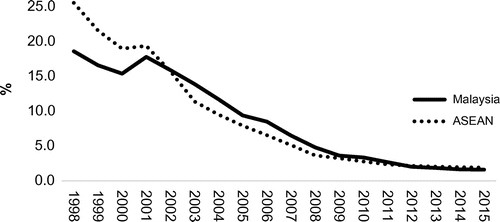
Since the Asian financial crisis, Malaysia has experienced a dramatically reducing trend in NPLs from 18.6 to 1.6%. This study will explore whether the risk of Malaysian banks, as measured by a CDD market model, follows a similar trend.

CDD is an extension of DD, which is based on a combination of the equity structure of a firm’s balance sheet, and fluctuations in market asset values. It essentially measures how a firm’s capital structure can be eroded when market asset volatility diminishes the distance between assets and liabilities, with the default point of the model being when asset values fall below liabilities. CDD is the author’s own novel metric, which has not before been applied to Malaysian banks, and provides a variation to DD in that it measures DD based on fluctuations found in the extreme tail of the asset value returns, thus showing how extreme fluctuations impact on default risk. In addition to the use of the CDD metric, this study includes a measure of the length of the tail risk (which we will term TR) by measuring the distance between asset value fluctuations under a DD model as compared to the CDD model. This provides a common size comparison of TR between credit portfolios and facilitates an understanding of Malaysia’s vulnerability to extreme market fluctuations relative to the ASEAN region.

DD is most commonly applied to the corporate customers of banks, however this study applies CDD to the Malaysian banks themselves. DD (or its underlying component of fluctuations in market asset values), applied to banks, has been identified by some central banks such as the European Central Bank (2005) and the Bank of England (2008) as a useful indicator of bank risk in that it identifies capital shortages. As market conditions deteriorate, it becomes more likely that assets need to be liquidated at market values, and DD can measure the erosion in capital that needs to be restored. In addition, because DD is based on market values, which can change daily, the metric provides an early warning indicator of risk. Blundell-Wignall and Roulet (2012) of the OECD found that an examination of the DD of banks can help to shed light on their policy and regulatory issues relating to aspects, such as leverage and funding.

The study also provides an analysis of the CDD of small vs. large banks. This question of the relationship between the size and risk of banks has been addressed by several authors with mixed findings. Stever (2007) found that smaller US banks are more risky than larger ones in that they are less diversified. This lack of diversity arises in a number ways, such as the smaller banks holding less loans, they have less diversity in borrower type, they have less access to large borrowers and they often have geographic restrictions, as smaller banks are generally more localised. Opposite to Stever’s findings, Laeven, Ratnovski, and Tong (2014), using data across a range of countries, found that large banks create more individual and systemic risk than small banks due to having characteristics such as less capital, less stable funding, more market-based activities and more organisational complexity. In contrast to both of these studies, Allen and Powell (2010) found no pattern of either higher or lower risk for small vs. larger banks when examining a number of a market and credit risk metrics over differing economic circumstances for banks in Australia, Canada, the US and the UK. In relation to Malaysia, Inoguchi (2012) found a link between size and credit risk, in that Malaysian banks with larger total assets had lower NPLs.

This study includes all listed local Malaysian banks available on Datastream, of which there are nine, over the 18-year period from 1998 to 2015. Comparisons are made to other countries in the ASEAN region. Specifically, the research questions are whether CDD and NPLs display similar trends, whether the TR of Malaysian banks changes over time, whether CDD differs between smaller and larger banks, and whether there are differences in these metrics between Malaysian Banks and the ASEAN region as a whole. The study will show that the risk of Malaysian banks has improved relative to ASEAN banks over the studied period across most of the metrics used, and that the risk of larger banks relative to smaller banks changes to a greater degree over crisis periods.

Given that this study examines a range of metrics including NPLs and the novel CDD and TR across smaller and larger banks, it provides a comprehensive picture of the credit risk of Malaysian banks and demonstrates how different measures can highlight different aspects of risk. The insights provided by this study can lead to an improved understanding of credit risk in Malaysia which is important to banks and regulators in determining capital adequacy, setting statutory requirements, making risk provisions and in identifying potential risks at an early stage. Given that the ASEAN economic community is moving towards banking integration within the region it is important to understand the relative risk of banks in the region, and this study contributes to the understanding of that risk for Malaysia, one of the pivotal countries in the ASEAN region, with 20% of the region’s private sector credit.

As far as we are aware, in a specifically Malaysian context, there are no studies using CDD at all, or applying CDD to small vs. large banks, or comparing TR of market asset value fluctuations, which are all extensions of this study to the literature and to the understanding of bank risk in Malaysia.

An additional contribution of the study is that our analysis will show that the extent and range of our data (85 banks over 18 years across 6 ASEAN countries) is much more extensive than the average range of data used by other similar studies on banks in Asia and in developing regions.

Following this introduction, some background is provided on Malaysian banks, then a framework for the study is developed which explores past literature and provides an explanation of the CDD and TR methodology and how they are incorporated into the study. The data and sample are then discussed, followed by an analysis of NPLs, CDD and TR. Given that CDD is an extension of DD, some comparisons will be made between our CDD outcomes as compared to what a DD measure would have revealed. Univariate and multivariate regression are then undertaken to establish the links between CDD size and returns, followed by conclusions.

2. Background on Malaysian banks

Bank Negara Malaysia (BNM) is responsible for prudential regulation and ensuring the safety and stability of the financial sector. Following the AFC, a 10-year Masterplan was implemented by BNM from 2001 to 2010, supplemented by a Capital Markets Masterplan. These initiatives saw a restructuring of the financial sector underpinned by a strong supervisory and regulatory framework. According to Bank Negara Malaysia (2016), there are 27 licensed commercial banks (19 of which are foreign), 19 Islamic Banks (3 of which are foreign) 11 investment banks and 2 other financial institutions.

Since the Asian financial crisis, the banking sector in Malaysia sector went through a period of consolidation with a substantial reduction in the number of financial institutions, and an improving trend in capital and NPLs. At 2015, the total risk-weighted capital ratio (TCR) of Malaysian banks was 16.9% and the risk weighted tier 1 capital ratio was 14.3%. These are well above Basel requirements. World Bank (2015) statistics show private sector debt at 125% of GDP and NPLs at 1.7%. Bank Negara Malaysia (2016) show gross impaired loans in the household sector of 1.1% compared to 2.5% for corporate debt. Malaysian banks are subject to regular stress tests and in recent years have been found to be able to withstand severe macroeconomic and financial shocks. Recent tests have applied two differing scenarios, the second a more prolonged stress scenario than the first, and under both scenarios the banking system is able to maintain Basel TCR, Tier 1 and Common Equity Tier 1 (CET 1) ratios above the minimum required level (Bank Negara Malaysia, 2015, 2016). A financial sector blueprint 2011–2021 was introduced to transform Malaysia’s financial sector to a high income, high value-added economy. Malaysia is working together with ASEAN countries to achieve greater market access and operational flexibility under the ASEAN Banking framework.

3. Development of a framework for CDD and TR

There are two key strands of literature on which the development of the framework for this study is based. The first relates to DD, which is important to explore as it is the model from which CDD is extended. DD is a market-based credit risk model which incorporates the volatility of market asset values and the distance between the asset and debt values of a firm. The second strand relates to the assessment of TR, which recognises that asset values have heavy tails which are not well captured by central measures of volatility such as standard deviation, and is the premise on which our CDD is formulated. These two strands, and the framework and methodology that we develop from them, are discussed separately in Sections 3.1 and 3.2 below. In these discussions of the literature, we will identify aspects such as methods used, length of time series samples and number of entities used in related studies, which will all help us develop our framework, as summarised in Section 3.3. In this study, we intend to analyse Malaysian banks as compared to the ASEAN region, for which we will use the six largest countries of Indonesia, Malaysia, Philippines, Thailand, Singapore and Vietnam which comprise 96% of the GDP of ASEAN countries. We have identified that between DataStream and World Bank that there is information which will adequately calculate CDD, TR and NPLs for 85 listed banks in the region, going back 18 years to 1998 which will include both the AFC and the GFC (although, being a developing region, the number of banks included in the sample for some of the comparison countries such as like Vietnam and Indonesia, becomes sparser the further back we go). A key part of the analysis in Sections 3.1 and 3.2 is to determine how adequate our proposed sample is in relation to other related studies that have been done globally and in Asia. What we find is that, while there are a small number of studies that exceed this proposed sample, these generally relate to developed markets such as Europe or the US where there is a wealth of data extending back many more years than developing ones like in the ASEAN region. We will show that our sample is well above the average for all global studies and far exceeds most samples used by other studies in Asia, particularly relating to developing countries.

3.1. Examination of studies on distance to default

DD as a measure of credit risk originated in the works of Black and Scholes (1973) and Merton (1974). It is based on option pricing methodology and a default event is triggered when market fluctuations in the asset values of a firm cause asset values to fall below the value of the firm’s debt. The Moody’s KMV model (Crosbie & Bohn, 2003), has become widely used by banks to measure the DD and probability of default (PD) of their customers.

Bharath and Shumway (2008) apply DD to US corporates from 1980–2003. In their study, the authors comprehensively set out the workings and formulae behind the Merton model, and it is these workings on which the CDD methodology in our study is based. We will first explain the calculations of a DD model and then explain how we modify it to arrive at CDD. Given that the workings are well covered in the Bharath and Shumway study, as well as in the work of Allen and Powell (2010), we will not repeat an explanation of these detailed workings of the model, but some key points are summarised here. The equation normally used to calculate DD is as follows:(1) $$\text{DD}=\frac{ln(A/D)+(\mathit{\mu }-0.5{\mathit{\sigma }}_A^2)T}{{\mathit{\sigma }}_A\sqrt{T}}$$(1)

A is the asset values of the firm. D is debt, calculated as short-term debt plus half of long-term debt (as explained in a subsequent paragraph below). μ is asset value drift. T is the forecasted time period which our CDD model sets to one year in line with usual DD practice. σ_A is the standard deviation of daily asset values. DD thus measures the number of standard deviations away from default, with a lower DD representing a higher default risk, and a DD of zero being the point of default.

To estimate σ_A, (from which our CDD is subsequently calculated), this study acquires daily equity values for each bank from which the standard deviation of the logarithm of daily price relatives is calculated. Then using these figures coupled with the liabilities of the firm, the model applies the estimation, iteration, convergence and correlation procedure explained in Bharath and Shumway (2008) and Allen and Powell (2010) to obtain asset values and daily asset returns for each individual bank in Malaysia (and for the comparison ASEAN countries), and for each country as a whole.

As explained in Vassalou and Xing (2004) and Allen and Powell (2010), there are some important variations of the KMV model from the Merton Model. Firstly, the Merton model uses a formula based on a standard normal distribution to calculate PD from DD. KMV instead uses their own empirical database of defaults to convert DD to EDF, an estimated default frequency. However, it is common in many studies which compare relative credit risk between entities or portfolios to use DD only (e.g. Blundell-Wignall & Roulet, 2012; Byström, Worasinchai, & Chongsithipol, 2005; Carlson, King & Lewis, 2008, Harada, Ito, & Takahashi, 2013). This is because PD is a derivation of DD, thus an entity with a lower DD (higher default risk) will always have a higher PD (higher default risk) irrespective of which method is used. Thus, our study only deals with the modified DD component (CDD) and not PD, and therefore this distinction in PD calculation methods is not material to us. Secondly, KMV holds that firms do not necessarily default when their assets fall below liabilities as long-term debt is not immediately due, and thus KMV uses current debt plus half of long-term debt. The model we use in this study follows the KMV approach in this regard in line with Vassalou and Xing (2004) and Allen and Powell (2010).

There are other studies which apply DD to corporates (as opposed being bank-specific), with some examples presented here. In a study that was applied to US corporates over the 13-year period from 2000–2012, Allen, Powell, and Singh (2016) found that a Merton type structural model which incorporates market asset value fluctuations is much more responsive to dynamic economic circumstances than macroeconomic or ratings based models, given that market-based models can respond quickly, even daily, to changing events. Also in relation to US corporates, Duffie, Eckner, Horel, and Saita (2009) over the 25-year period from 1979–2004 found that DD can explain a large part of the variation in default risk between companies and across time periods, but the authors find that it cannot on its own completely account for default intensity. Byström et al. (2005) used DD to examine the default risk of 50 Thai firms, including several banks, over the 8-year period 1996–2003 before, during and after the Asian crisis, finding that market-based default probabilities increased substantially during the crisis and were slow to return to pre-crisis levels. The authors also examined the relationship between DD, returns, size and market to book by dividing their portfolio into “bottom”, “mid” and “top” bands according the size of the DD and comparing the market to book, size (by market cap) and returns associated with the firms in each of these band, as well using multiple regression to determine the relationship between the variables. Over the whole period they do not find significant association between default risk and the other variables, but do find a size effect over the crisis period only (smaller firms being the most distressed). A further study which included size and market to book effects (also using different bands to categorise default levels, as well as regressions) was Vassalou and Xing (2004) in a study of from 1971–1999 of 4,250 US corporates, which finds both effects to be related to default risk, whereby small firms (and value stocks) earn higher returns than big firms (and growth stocks), only if they also have high default risk. In line with these studies, our study will assess size and market to book effects in a regression equation.

Allen, Boffey, Kramadibrata, Powell and Singh (2013) used DD over the 6-year period 2005–2011 to demonstrate that the relatively high capital of 217 Indonesian Agriculture and Mining firms makes them resilient to fluctuating asset values.

Bank Negara Malaysia (2008) used DD (together with NPLs and z score) over the 5-year period 2004–2008 on 230 corporates listed on the Bursa Malaysia, to demonstrate how the structural, operational and financial reform measures instituted after the Asian crisis led to improved credit risk, even during the global financial crisis period of 2008.

In relation to sovereign risk in Asia, Unurjargal and Bernard (2015) used DD to measure excess sovereign credit risk prior to the financial crisis. They found that while some Asian countries exhibited signs of excess debt prior to the crisis, Malaysia and Indonesia did not.

We will now examine some studies which apply DD specifically to banks. Chan-Lau and Sy (2006) from the International Monetary Fund, apply a modified DD model (which they term distance to capital) to two distressed Japanese Banks over the period 2001–2003. They find that such market-based measures of capital adequacy can be useful in helping to identify capital shortages, thus allowing corrective supervisory action to be taken before a bank default.

Harada et al. (2013) investigated the predictive power of the Merton DD measure for bank failures, based on eight failed Japanese banks, finding that DD was generally a reliable indicator of bank failure, becoming smaller in anticipation of failure in many cases. Where this did not happen it indicated lack of public information partly due to insufficient transparency in financial statements. The study took place over eight years from 1986 to 1998, providing a particular focus on the DD in the six months prior to failure.

Boumediene (2011) used DD to show that Islamic banks have lower credit risk than conventional banks in a study of nine banks over the 5-year period from 2005–2009.

The European Central Bank (2005) applied DD to major banks in the Euro area for the 13 years from 1992–2004. They expressed the view that market-based indicators like the DD model are a good complement to balance sheet indicators as they are forward looking and can shed light on perceptions of the robustness of the financial system.

Powell and Vo (2016) incorporate NPLs, DD, Capital and other risk metrics as part of the formulation of stress indicator models for the 85 listed banks in ASEAN countries. Allen and Powell (2010) applied DD to 149 banks in Australia, US, Europe and Canada over the 10 years from1999–2008 and find that the model identifies significantly higher risk in market value volatility than is evident in balance sheet book values. Using regression, they found a relationship between size and risk for US banks, but not for the other regions.

A further bank study which incorporated size as a regression variable was Blundell-Wignall and Roulet (2012), who used a Merton DD model on 94 US banks over eight years from 2004–2011, and found that, when excluding globally systemically important financial institutions (G-SIFI), from their sample of large banks, size appears not to matter as a determinant of DD.

3.2. CDD and TR

The second strand of our framework deals with TR. Many studies focus on tail estimations, due to the well-known feature of heavy tails in many asset returns. Examples include the relationship of fat tails to volatility long-range correlations (Bacry, Kozhemyak, & Muzy, 2006), extreme value theory which looks at high deviations from the mean of probability distributions (McNeil & Frey, 2000), quantile regression which models conditional quantiles of a variable such as the 95th percentile, and studies which measure VaR, CVaR and CDD as discussed below.

CDD originated in the PhD thesis of Powell (2007) and is contained in various subsequent works (such as Allen et al., 2016; Allen & Powell, 2010). It is based on the concepts of tail risk measures such as value at risk (VaR) and conditional value at risk (CVaR), which in turn is an extension of VaR. VaR is widely used as a measure of market risk. It measures the maximum loss that occurs through asset value volatility up to a specified threshold, such as 95%. CVaR on the other hand measures those losses beyond VaR. If VaR is measured at 95%, then CVaR is the average of the worst 5% of returns. While VaR and CVaR have primarily been used as measures of market risk, they have also been used in various credit risk studies, primarily applied to optimisation and transition matrices, such as Andersson, Mausser, Rosen, and Uryasev (2000), Uryasev and Rockafellar (2000), Allen and Powell (2009) Powell and Allen (2009) and Allen et al. (2016). In a similar vein to VaR and CVaR, CDD measures asset volatility at (or beyond) a selected high threshold and this study measures it at the 95% level of asset value returns, which is termed CStdev. Equation 1 is then modified to obtain CDD in equation 2 as follows:(2) $$\text{CDD}=\frac{ln(A/D)+(\mathit{\mu }-0.5{\mathit{\sigma }}_A^2)T}{\text{CStdev}\sqrt{T}}$$(2)

A metric incorporated in this study is TR of market asset value fluctuations. While there have been measures of tail length of items such as equities or commodities in the literature relative to a normal or other specified distribution benchmark (Embrechts, Puccetti, Rüschendorf, Wang, & Beleraj, 2014; Powell, Vo & Pham, 2017), this is the first measure of which we are aware which applies it to credit risk in Malaysia in terms of measuring the distribution of market asset values as contained in the denominator of the DD equation relative to CDD:(3) $$\text{TR}=\text{Cstdev}/{\mathit{\sigma }}_A$$(3)

This metric provides an indication of the normality of the tail length of the market asset values. Under a normal distribution assumption, using standard normal tables, standard deviation (σ) = 1 and the 95% return (on which Cstdev in this study is based)=1.645. Thus, TR > 1.645 indicates a longer tail than a normal distribution and TR < 1.645 a shorter tail. We examine TR over time, to see whether tail length changes in different periods (such as in crisis and non-crisis periods), and whether there are differences in tail length between ASEAN and Malaysian Banks.

3.3. Summary of studies

In the review of prior studies above, it has been determined that our study will include CDD and TR, and the methodologies behind calculating these have been identified. We have proposed in our introduction that the study will also establish the relationship between size and CDD for the banks in the sample. The literature has shown that there are a number of studies which use regression (Allen & Powell, 2010; Bharath & Shumway, 2008; Blundell-Wignall & Roulet, 2012; Byström et al., 2005; Vassalou & Xing, 2004) and division of firms into panels according to size of DD and its associated explanatory items (Byström et al., 2005; Vassalou and Xing, 2004). The panel and regression methodolgy of Byström et al. (which has some similarities to Vassalou and Xing) will be followed, given that it is the only one of these studies undertaken in a developing area (Thailand).

Table 1 summarises the sample sizes of prior studies, which we acknowledge are all perfectly suitable sample sizes for the particular focus of each of these studies. On average, these prior DD studies cover 2 countries or regions, have 61 banks in the sample, and include 13 years of data. However, this is a mix of developed and developing regions. Our study is in a developing region, where markets are much newer and which don’t have the same level of data as developing regions. In particular, the average figures below are increased by studies in the US. On average, studies in developing areas or in Asia include 2 countries or regions, 29 banks and 9 years in the sample.

Table 1. Sample size of prior studies

Study	Country/region	No. countries or regions in sample	Developed or developing region	No. banks in sample	Years	No. of years	Topic
(a) Studies applying DD to banks
This study	Malaysia, plus five ASEAN countries	6	Developing	85	1998–2015	18	DD, CDD, TR
Allen and Powell (2010)	Australia, US, Europe, Canada	4	Developed	149	1999–2008	10	DD, CDD
Blundell-Wignall and Roulet (2012)	Europe Canada US	3	Developed	94	2004–2011	8	DD
Carlson et al. (2011)	US	1	Developed	68	1973–2007	35	DD
Chan-Lau and Sy (2006)	Japan	1	Developed	2	2001–2003	3	DD
Boumediene (2011)	Asia	1	Developing	9	2005–2009	5	DD
European Central Bank (2005)	Europe	1	Developed	Unspecified	1992–2004	13	DD
Harada et al. (2013)	Japan	1	Developed	19	1985–2005	21	DD
Powell & Vo (2016)	Asean	6	Developed	85	1985–2005	10	DD
(b) Studies applying DD to non-banks
Allen et al. (2016)	US	1	Developed	–	2000–2012	13	DD, CDD
Bharath and Shumway (2008)	US	1	Developed	–	1980–2003	24	DD
Bank Negara Malaysia (2008)	Malaysia	1	Developing	–	2004–2008	5	DD
Byström, Worasinchai & Chonsithipol	Thailand	1	Developing	–	1996–2003	8	DD
Duffie et al. (2009)	US	1	Developed	–	1979–2004	25	DD
Vassalou and Xing (2004)	US	1	Developed	–	1971–1999	29	DD
Average		2		64		15

The data proposed in this study, as discussed in Section 4 below cover 6 countries, 85 banks and 18 years of data. This well exceeds the average of all studies and more importantly is close to a full sample in that it includes all the six major countries in the ASEAN region (which comprise 96% of the region’s GDP), all the listed banks in the region, and goes back as far as it is possible to adequately calculate CDD and TR and to provide valid comparisons for the selected countries (we note that the number of banks in the more developing countries in our comparison ASEAN sample, such as Vietnam and Indonesia, reduces the further back we go, and beyond 18 years, the data become too sketchy for adequate analysis).

4. Data and sample

Having established the size of our data sample in relation to other studies, particularly those in Asian and developing areas, we will now provide more details on our data.

The CDD, TR and regression models in this study are used to examine all listed Malaysian commercial banks that are available on Datastream, of which there are nine. These include (in order of asset size) Malayan Bank, CIMB, Public Bank, RHB Bank, Hong Leon, Ambank, Affin, BIMB and Alliance. The total assets of these banks in 2016 are RM 2,125 billion (USD 510 billion). For purposes of comparing larger and smaller banks in this sample, we will classify the first four banks mentioned above as large. These large banks each have assets exceeding RM 200 billion with aggregate value of RM 1.6 trillion and average value of RM 408 billion. The other five banks are classified as small. These small banks all have assets less than RM 200 billion, with an aggregate value RM 490 billion and an average value of RM 98 billion.

The study will also compare NPLs and CDD for Malaysia to other countries in the ASEAN region. Our comparison includes the six countries of Indonesia, Malaysia, the Philippines, Singapore, Thailand and Vietnam, which represent 96% of total GDP in the ASEAN region, and our sample incorporates 85 banks across these countries. We will also compare Malaysian Banks to the ASEAN region as whole, being the average NPL and CDD of these six countries.

All the data required to undertake the CDD modelling are obtained from Datastream. This includes 18 years of daily equity prices for each of the 9 banks as well as debt and asset balance sheet data. NPL information is obtained from a combination of World Bank (2015) data and BNM (Bank Negara Malaysia, 2016) statistics.

5. Analysis and results

This section will present, analyse and discuss various sets of figures and results relating to bank risk in Malaysia, including NPLs, CDD, TR and regressions. Tables 2–3 compare the current period for the first two of these items to the AFC and GFC crisis periods. Our data show that most of the negative impact to bank risk of these two crises occurred around two-year periods (1998–1999 for AFC and 2008–2009 for GFC), thus it is these two-year periods that we use in the tables. To keep an equal two-year length of comparison for our current period, we use the two most recent years of available data (2014–2015). The study then examines annual trends in the risk metrics, including a comparison of smaller vs. larger banks.

Table 2. NPLs of ASEAN countries. Current compared to crisis periods

Country	AFC	Rank	GFC	Rank	Current	Rank
Indonesia	40.8	4	3.2	3	2.2	4
Malaysia	17.6	3	4.2	5	1.6	2
Philippines	13.5	2	4.1	4	2.0	3
Singapore	5.3	1	1.7	1	0.8	1
Thailand	40.8	4	5.5	6	2.5	5
Vietnam	–	–	2.0	2	2.9	6
Average ASEAN	23.6		3.5		2.0

Table 3. CDD of ASEAN countries. Current compared to crisis periods

Country	AFC	Rank	GFC	Rank	Current	Rank
Indonesia	0.5	5	1.2	2	1.5	5
Malaysia	0.8	3	1.3	1	2.2	1
Philippines	1.0	2	1.1	3	2.0	2
Singapore	1.0	1	0.9	5	1.9	3
Thailand	0.6	4	1.0	4	1.5	6
Vietnam	–	–	0.7	6	1.7	4
Average ASEAN	0.8		1.0		1.8

5.1. NPL analysis

One of the strategies introduced by some ASEAN countries for reducing NPLs (loans where payment of interest and principal is past due by 90 days or more) after the Asian crisis was to set up public asset management companies to purchase NPLs from banks. Examples include the Thai Asset Management Corporation in Thailand and the Pengurusan Danaharta Nasional Berhad in Malaysia. Inoguchi (2012) found that these strategies did have some impact on reducing NPLs. This was particularly the case in Thailand. In Malaysia, NPLs actually went up over the short NPL purchasing period after the crisis, but Ignoguchi found that the situation would have been worse without these purchases and could not deny that these asset purchases had some impact. Inoguchi also found that improving macroeconomic conditions had an impact on reduction of NPLs in Malaysia and Thailand.

Table 2 compares and ranks NPLs (as a percentage of gross loans) between six ASEAN countries. A ranking of 1 indicates the lowest NPL risk among the countries, and 6 is the highest risk. It shows how average NPLs in the region have reduced dramatically from 23.6% during the AFC to 2.0% currently. In Malaysia, the reduction was from 17.6% to 1.6%. Malaysia’s ranking among ASEAN countries slipped from 3 to 5 between the AFC and GFC and has since improved to 2. Singapore has consistently displayed the lowest NPL risk. Figures were not available for Vietnam in 1998–1999.

In 1999, Malaysia NPLs ranked 66th out of 84 global countries (79th percentile). In 2015 Malaysia’s position had improved to 23 out of 120 global countries (19th percentile). It is interesting to make comparisons with the United States, who had a far lower NPL percentage (1.0%) than Malaysia (16.6%) in 1999 and the US had a similar percentage (1.5%) to Malaysia (1.7%) in 2015.

Figure 1 compares the trend of Malaysian NPLs to ASEAN NPLs. It shows that Malaysian NPLs have reduced at a faster rate since the GFC than the ASEAN ones. The ASEAN trend has plateaued in recent years.

Figure 1. NPL to gross loans % trend 1998–2015: Malaysia compared to ASEAN Countries.

5.2. CDD and TR analysis

Table 3 compares CDD for Malaysian banks to the ASEAN region for the AFC, GFC and current period. The CDD ranking for Malaysian banks improves from 3 (AFC) to 1 (GFC and Current) over the period.

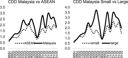
The trends in these CDD figures for all 18 years are shown in the first chart in Figure 2. To highlight the trends, a smoothed line has been used. It is clear that Malaysia (with minor exception around 2004/2005) has a consistently higher CDD (lower risk) than the ASEAN average. Figure 2 shows that CDD increased prior to the GFC in ASEAN as well as Malaysia. The exception in around 2004/2005, where Malaysia showed a lower CDD (higher credit risk) than ASEAN, was a period where some of the other ASEAN countries (notably Indonesia and Thailand) had experienced a substantial fall in credit risk which was reflected in their higher CDD. Indonesia and Thailand both had NPLs of over 40% during the AFC, thereafter introducing stringent reforms into their banking sectors, including the closure or merger of several banks and the tightening of capital and credit regulations. Indonesia’s NPL’s had reduced to 7.3% in 2005 and Thailand’s to 9.1% compared to Malaysia’s 9.4%. This, coupled with Singapore’s constantly low NPL’s in 2005, caused CDD to show a lower risk for ASEAN over this period. Malaysia’s more steady overall NPL performance soon returned its CDD to levels above ASEAN.

Figure 2. CDD trends 1998–2015.

The fluctuation of the market asset values of an entity is an important component of the CDD and is shown in Table 4. Here, there are substantial differences between Malaysia and the ASEAN average. Indeed, the average Cstdev (the fluctuating component of CDD per the denominator of equation 2(2) $$\text{CDD}=\frac{ln(A/D)+(\mathit{\mu }-0.5{\mathit{\sigma }}_A^2)T}{\text{CStdev}\sqrt{T}}$$(2) ) for Malaysian banks over the 18-year period (0.053) is approximately half that of the ASEAN average (0.010). The final column of Table 4 provides our TR measure (Cstdev/σ_A which are the fluctuating components of CDD and DD, respectively, per equations 2 and 1) of the length of the tail of the asset value distribution. The distribution for Malaysia over the studied period ranges between 1.119 and 1.884 as compared to ASEAN which ranges between 1.412 and 1.818. Malaysia’s TR is notably lower than ASEAN in 1998 at the time of the AFC (when their NPL’s were also lower than ASEAN) and notably higher than ASEAN in 2008 at the time of the GFC (when their NPL’s are also higher than ASEAN).

Table 4. Measures of asset volatility 1998–2015: Malaysia compared to ASEAN Countries

Year	Cstdev Malaysia	Cstdev ASEAN	TR (Cstdev/σA) Malaysia	TR (Cstdev/σA) ASEAN
1998	0.132	0.246	1.119	1.444
1999	0.091	0.202	1.486	1.464
2000	0.070	0.173	1.548	1.674
2001	0.069	0.194	1.417	1.818
2002	0.055	0.112	1.707	1.469
2003	0.035	0.102	1.210	1.418
2004	0.042	0.091	1.391	1.443
2005	0.042	0.068	1.810	1.439
2006	0.043	0.075	1.660	1.508
2007	0.051	0.096	1.311	1.513
2008	0.094	0.157	1.884	1.730
2009	0.035	0.071	1.512	1.412
2010	0.024	0.075	1.356	1.598
2011	0.038	0.073	1.749	1.606
2012	0.024	0.057	1.699	1.622
2013	0.027	0.077	1.400	1.550
2014	0.031	0.050	1.619	1.527
2015	0.047	0.063	1.698	1.662
Average	0.053	0.110	1.532	1.550

Although we have focussed on CDD in this study, it is important to comment on how our results differ from those we would have achieved had we used DD. Using equation 1 we found that, when we applied it to all the years in our sample, that DD and CDD patterns follow each other quite closely, albeit with CDD at a lower level. In fact, if we compare TR (which essentially measures the gap between DD and CDD) for the GFC years (2008–2009) with the pre-GCF years (2002–2007), they are very close together (averaging close to 1.5 for both Malaysia and ASEAN in both periods), indicating a reasonably constant gap between DD and CDD for these periods. The question that could then be raised is whether CDD provides any information to banks and regulators that is different to DD. In fact, this similarity provides a great deal of important information. Most studies (usually relating to the US) using VaR and CVaR type measures find large differences in patterns between these metrics and standard deviation for banks over the GFC as compared to the pre-GFC. For example, Allen and Powell (2010) showed changing patterns in the gaps between DD and CDD for Europe, the US and even Australia from the pre-GFC to GFC period. These stable patterns in Malaysia and the ASEAN region are therefore different to what has been found in other areas, and reflect the views of the market on the relative stability of Malaysian and ASEAN banks, which together with the decreasing NPLs, can provide some confidence to the banks and regulators in the reforms that have been made.

The analysis now turns to a comparison of large and small Malaysian banks (as mentioned previously, the large sample comprises the largest four banks, and the small sample comprises the smallest five banks). It is evident from the second chart in Figure 2 that size plays a factor, with CDD for smaller banks trending for the most part below (higher risk) that of larger banks. The large banks had a CDD average over the period of 2.19 compared to 1.61 for small banks. We note though, that while the group of larger banks had a lower risk for CDD than the group of smaller banks, the pattern was not entirely consistent for individual banks, i.e. the largest bank in the large sample did not necessarily have the lowest risk out of the large bank sample nor the smallest bank in the large sample the highest risk out of the large sample. The same applied to the small sample.

However, although overall the larger banks had a lower risk for CDD than smaller banks, the graph shows that this changes in crisis periods, with CDD for larger banks moving much closer to that of smaller banks. In 1998 at the time of the AFC, the CDD for smaller Malaysian banks was 0.6. This was very close to the CDD (0.7) of larger banks. A similar phenomenon happened in 2008 when CDD for larger banks (0.9) in fact fell below that of smaller banks (1.0). Yet in the non-crisis periods, CDD demonstrated much lower risk for larger banks than for smaller ones. In 2012, CDD peaked at 3.5 for larger banks yet only reached 2.5 for smaller banks. Thus, while smaller banks in Malaysia are generally perceived as riskier than larger banks for most of the time, in crisis times there is a loss of confidence in larger banks with a corresponding plummet in their asset values and CDD down to the level of smaller banks. Therefore, while smaller banks in Malaysia have a higher risk most of the time, there is more stability in their risk levels across periods than for larger banks. This also results in greater stability in the shape of the asset value distribution with the average TR of smaller banks (1.39) being lower than of larger banks (1.75). For our ASEAN region as a whole, there was a slightly different picture. Although larger banks also had a consistently higher CCD than smaller ones, this was less pronounced, and we will see when it comes to the regression equations, that this difference was less statistically significant for ASEAN than for Malaysia. In particular, there was lesser variation in default statistics in non-crisis periods and not the same degree of narrowing in the ASEAN default metrics during crisis periods.

5.3. Regressions

To show the relationship between size, CDD, returns and MTB, similar to the Byström et.al study we mention in Section 3.3, we divide our portfolio into cross sections according to size, for which we use small and large. These results are presented in Table 5. Consistent with Byström et al., we calculate the daily average of figures for every month for CDD, market to book (MTB) and market capitalisation (Size). The monthly return figure is based on subsequent returns for the ensuing 12 months. The figures for each period are based on the average monthly figures for that period. We use the 1998–1999 AFC and the 2008–2009 GFC as our crisis period and all other years as our non-crisis period. It is immediately apparent from Table 5, confirming what we showed in Figure 2, that larger banks (which in this sample also have larger MTB values) have lower credit risk in terms of CDD, for both Malaysian and ASEAN Banks, across crisis and non-crisis periods. But there is no apparent relationship between CDD and returns. This finding is consistent with Byström who notes that, given that higher default probabilities are not rewarded by higher returns this would indicate that default risk is idiosyncratic and not systematic. We cross-checked whether we would obtain the same regression results if we had used DD instead of CDD, and found very similar relationships for both ASEAN and Malaysia, again highlighting the relative tail stability of credit risk in this region.

Table 5. Relationship between CDD, Size, MTB and Returns

	Malaysia		ASEAN
	Small	Large	Small	Large
Total period
CDD	1.61	2.19	1.30	1.51
Size	1,385	6,744	167	3,590
MTB	1.28	1.64	1.62	1.76
Returns	−0.030	−0.044	0.014	0.011
Crisis periods
CDD	0.99	1.14	0.83	0.98
Size	887	5,057	128	3,039
MTB	1.96	2.15	1.67	2.19
Returns	−0.151	−0.198	0.014	−0.006
Non-crisis periods
CDD	1.84	2.58	1.53	1.59
Size	2,089	10,152	252	5,422
MTB	1.88	2.56	2.30	2.62
Returns	−0.018	−0.034	0.022	0.017

Added to the above analysis, like Byström, we also undertake univariate (CDD as the dependent variable and Size as the independent variable) and multiple regression analysis, using the same data as for the cross-sectional analysis above with returns (for the subsequent year) as the dependent variable ret-1y, and the independent variables CDD, Size and MTB.(4) $$\text{ret -1y}=a_{0,t}+a_{1,t}CDD+a_{2,t}\text{Size}+a_{3,t}\text{MTB}+{\mathit{\epsilon }}_t$$(4)

Consistent with Byström, we calculate regressions for every month in our sample (216 regressions, being 12 months × 18 years) and the coefficients presented in Table 6 are the average of the 216 regressions.

Table 6. Regression: returns against MTB, Size and CDD

Malaysia	Multiple regression returns against MTB, Size and CDD					Single regression CDD against Size
		MTB	Size	CDD	Intercept	Size	Intercept
Total period	Coeff.	0.010707	0.000019	0.063620	0.004589	0.000191	1.24
	Sig.	–	–	–	–	*	**
Crisis	Coeff.	0.003544	0.000058	0.190090	0.056953	0.000129	0.81
	Sig.	–	–	–	–	–	**
Non-crisis	Coeff.	0.012374	0.000007	0.024964	0.022822	0.000202	1.46
	Sig.	–	–	–	–	**	**
ASEAN	Multiple regression returns against MTB, Size and CDD					Single regression CDD against Size
		MTB	Size	CDD	Intercept	Size	Intercept
Total period	Coeff.	0.004899	0.000001	0.002738	0.007708	0.000040	1.22
	Sig.	–	–	–	–	–	**
Crisis	Coeff.	0.021600	0.000000	0.005374	0.007502	0.000063	0.52
	Sig.	–	–	–	–	–	**
Non-crisis	Coeff.	0.000119	0.000001	0.001684	0.013433	0.000038	1.39
	Sig.	–	–	–	–	–	**

* Denotes 5% significance.

** Denotes 1% significance.

– Denotes no significance.

For the univariate analysis, we confirm the strong relationship between size and CDD for Malaysia, with significance at 95% for the entire period, 99% for non-crisis period but < 95% for the crisis period. This lesser relationship during the crisis period is due to the gap in default statistics narrowing between smaller and larger banks—as we have mentioned previously, smaller banks are usually perceived as higher risk, but during crisis periods, larger banks also became perceived as risky, thus narrowing the gap between the default statistics of the two sets of banks. In the ASEAN region as a whole, although we found a relationship between size and default in our cross-sectional analysis, the significance of this relationship was found to be < 95% for all periods in the univariate regression.

For the multivariate analysis, for both ASEAN and Malaysian banks, we found no significance between returns and the independent variables in either the crisis and non-crisis periods, again providing evidence that default risk is not systematic, as if it was, we would expect that high default risk is compensated for by higher returns. The multivariate analysis has very similar findings to what Byström found for Thai Banks only, although Byström did find some size effects during the crisis, which we did not find, however Byström used a lower level of significance (90%) than this study (95%).

6. Conclusions

The research questions set at the start of this study are whether CDD and NPLs display similar trends, whether the TR of Malaysian banks changes over time, whether these factors differ between smaller and larger banks, and how Malaysian banks compare to the ASEAN region. The study showed that NPLs for Malaysian banks displayed a consistent downward (improving) trend, whereas CDD had a deteriorating trend over the GFC. This is because market factors in crisis periods are often influenced by global trends, most notably the dramatic events in the United States over the crisis period, rather than by fundamentals such as NPLs. Thus, although Malaysian banks had no increase in NPLs, the market values of the banks deteriorated quite markedly. This is consistent with the article mentioned earlier in this study by Allen and Powell (2010), who found a similar phenomenon among Australian banks.

NPL’s for Malaysian Banks increased above the ASEAN region between the AFC and GFC, but subsequently reduced at a faster rate than for the ASEAN region. CDD stayed consistently lower than the ASEAN region. The average tail length of Malaysian banks as measured by Cstdev/σ_A, was relatively similar to the ASEAN region. In regard to smaller and larger banks, the study found that smaller Malaysian banks exhibited greater risk than the larger banks as measured by CDD during non-crisis periods but there was a lesser degree of difference in risk during crisis periods. This outcome for non-crisis periods supports the findings of the previously mentioned Inoguchi (2012) study who found that smaller banks in Malaysia had higher risk, as measured by NPLs, than larger banks, but shows a different picture for crisis periods. The shape of the asset value distribution in terms of TR, was found to be more stable for smaller banks. In regard to returns, it was found that default risk was idiosyncratic, as if it was systematic, a higher default risk would be compensated for by higher expected returns. Overall, the reduction of risk in the Malaysian banking sector is a good sign for the ASEAN region as the countries within the region move towards greater financial integration.

Funding

The author received no direct funding for this research.

Acknowledgements

The author thanks the editor and two anonymous referees for their very helpful comments in improving the paper.

Additional information

Notes on contributors

R.J. Powell

R.J. Powell is an associate professor in Finance at Edith Cowan University. He has a PhD and lectures and researches in banking and finance. He is a director of the Markets and Services Research Centre, a cross-disciplinary centre researching in services industries, marketing, tourism and finance. This paper on Malaysia forms part of a series of projects of extreme risk in equity, commodity and credit markets, with a recent focus on the ASEAN region. He has 20 years banking experience in South Africa, New Zealand and Australia. He has been involved in the development and implementation of several credit and financial analysis models in banks.

References

- Allen, D. E., & Powell, R. J. (2009). Transitional credit modelling and its relationship to market at value at risk: An Australian sectoral perspective. Accounting and Finance, 49, 425–444.10.1111/acfi.2009.49.issue-3
- Allen, D. E., & Powell, R. J. (2010). The fluctuating default risk of Australian banks. Australian Journal of Management, 37, 297–325.
- Allen, D. E., Powell, R. J., & Singh, A. K. (2016). Take it to the limit: Innovative CVaR applications to extreme credit risk measurement. European Journal of Operational Research, 249, 465–475.10.1016/j.ejor.2014.12.017
- Andersson, F., Mausser, H., Rosen, D., & Uryasev, S. (2000). Credit risk optimization with conditional value-at risk criterion. Mathematical Programming, 89, 273–291.
- Bacry, E., Kozhemyak, A., & Muzy, J.-F. (2006). Are asset return tail estimations related to volatility long-range correlations. Physica A: Statistical Mechanics and its Applications, 370, 119–126.10.1016/j.physa.2006.04.022
- Bank Negara Malaysia. (2008). Financial stability and payment systems report.
- Bank Negara Malaysia. (2015). Financial stability and payment systems report.
- Bank Negara Malaysia. (2016). Statistics. Retrieved from http://www.bnm.gov.my
- Bank of England. (2008, October). Financial stability report.
- Bharath, S. T., & Shumway, T. (2008). Forecasting default with the merton distance to default model. The Review of Financial Studies, 21, 1339–1369.10.1093/rfs/hhn044
- Black, F., & Scholes, M. (1973). The pricing of options and corporate liabilities. Journal of Political Economy, 81, 637–654.10.1086/260062
- Blundell-Wignall, A., & Roulet, C. (2012). Business models of banks, leverage and the distance-to-default. OECD Journal: Financial Market Trends, 2012, 7–34.
- Boumediene, A. (2011). Is credit risk really higher in Islamic banks? The Journal of Credit Risk, 7, 97–129.10.21314/JCR.2011.128
- Byström, H., Worasinchai, L., & Chongsithipol, S. (2005). Default risk, systematic risk and Thai firms before, during and after the Asian crisis. Research in International Business and Finance, 19, 95–110.10.1016/j.ribaf.2004.10.005
- Carlson, M. A., King, T., & Lewis, K. (2011). Distress in the financial sector and economic activity. The BE Journal of Economic Analysis & Policy, 11, 1–31.
- Chan-Lau, J. A., & Sy, A. N. (2006). Distance-to-default in banking: A bridge too far (IMF Working Paper No. WP06/215).
- Crosbie, P., & Bohn, J. (2003). Modelling default risk. Moody’s KMV Company Report.
- Duffie, D., Eckner, A., Horel, G., & Saita, L. (2009). Frailty correlated default. Journal of Finance, LXIV, 64, 2089–2123.10.1111/j.1540-6261.2009.01495.x
- Embrechts, P., Puccetti, G., Rüschendorf, L., Wang, R., & Beleraj, A. (2014). An academic response to basel 3.5. Risks, 2, 25–48.10.3390/risks2010025
- European Central Bank. (2005, June). Financial stability review.
- Harada, K., Ito, T., & Takahashi, S. (2013). Is the distance to default a good measure in predicting bank failures? A case study of Japanese major banks. Japan and the World Economy, 27, 70–82.10.1016/j.japwor.2013.03.007
- Inoguchi, M. (2012). Nonperforming loans and public asset management companies in Malaysia and Thailand. Asia Pacific Economic Papers, 398, 1–37.
- Laeven, L., Ratnovski, L., & Tong, H. (2014, May). International monetary fund staff discussion note SDN 14/04.
- McNeil, A., & Frey, R. (2000). Estimation of tail related risk measure for heteroscedastic financialtime series: An extreme value approach. Journal of Empirical Finance, 7, 271–300.10.1016/S0927-5398(00)00012-8
- Merton, R. (1974). On the pricing of corporate debt: The risk structure of interest rates. Journal of Finance, 29, 449–470.
- Powell, R. J. (2007). Industry value at risk in Australia (PhD dissertation). Edith Cowan University.
- Powell, R. J., & Allen, D. (2009). CVaR and credit risk management. In 18th World IMACS Congress and MODSIM09 International Congress on Modelling and Simulation, 1508–1514. Cairns.
- Powell, R. J., & Vo, D. H. (2016). Road rules for a stress indicator model in a developing region (Working Paper). Edith Cowan University.
- Powell, R. J., Vo, D. H., & Pham, T. N. (2017). Economic cycles and downside commodities risk. Applied Economics Letters, 1–6. doi:10.1080/13504851.2017.1316818
- Stever, R. (2007). Bank size, credit and the sources of bank market risk. Bank for International Settlements (Working Paper No. 238). Basel.
- Unurjargal, N., & Bernard, L. (2015). A quantitative approach to assessing sovereign default risk in resource-rich emerging economies. International Journal of Finance and Economics, 20, 220–241.
- Uryasev, S., & Rockafellar, R. T. (2000). Optimization of conditional value-at-risk. Journal of Risk, 2, 21–41.
- Vassalou, M., & Xing, Y. (2004). Default risk in equity returns. Journal of Finance, 59, 831–868.
- World Bank. (2015). Data. Retrieved from http://data.worldbank.org/