Is stock market overpriced? A benchmark approach

Abstract

The fact that stock market is unpredictable does not deter investors, pundits, and academicians from speculating about the next market move. This paper uses multiple benchmarks to judge the current level of the stock market. Among those benchmarks are bonds; commodities; REITs; international stocks; company earnings, sales, and profits; and GDP. Ten-year moving averages of benchmark variables are individually and then collectively compared with S&P 500 index. Although our analysis finds that fundamentals do not support the current high level of the stock market, we do find evidence that a rational bubble exists in that market using the duration dependence test.

Keywords:

• Standard and Poor’s 500 index (SPX)
• duration dependence test
• CAPE

PUBLIC INTEREST STATEMENT

The fact that stock market is unpredictable does not deter investors, pundits, and academicians from speculating about the next market move. This paper uses multiple benchmarks to judge the current level of the stock market. Stock values cannot increase forever without an economic justification. If the prices of alternative investment vehicles are flat, the stock prices should not be able increase also. Among those alternatives are bonds; commodities; REITs; international stocks; company earnings, sales, and profits; and GDP. Ten-year moving averages of benchmark variables are individually and then collectively compared with S&P 500 index. Our analysis finds that economic fundamentals do not support the current high level of the stock market. Investors should be cautious and diversify their investment with alternatives to the stock market.

1. Introduction

The behavior of the U.S. stock market since March 2009 has clearly enriched those invested in it. The recent series of consecutive record highs across all major indexes has generated demonstrable angst among investors who realize that the bull market could continue for years or collapse any day. Investors are conflicted between a realization that stocks are pricey and a concern for opportunities lost should they take gains prematurely, i.e., the classic fear versus greed conundrum. This paper investigates whether fundamentals support the current stock market level by benchmarking the stock market levels against multiple macro and micro variables. Regardless of our conclusions, we cannot solve the investor’s dilemma. We can only hope to provide useful insight into market valuation.

The macro benchmarks we use include alternative investment classes such as bonds, commodities, foreign equities, and real estate as well as economic indicators such as GDP, inflation, money supply, interest rates, unemployment rates, and industrial production index (IPI). Micro benchmark variables include aggregate company earnings, sales, assets, and dividends. Ultimately, these benchmarks will be used to create a single metric for comparison with the current level of the stock market.

Several previous studies have discussed the mean reversion of market multiples to long-term average levels (e.g., see Coakley & Fuertes, 2006). Some papers confirm that mean reversion does occur, but note that long-term fundamental averages appear to shift over time. In other words, the “normal” level for a market multiple can change (e.g., see Balke & Wohar, 2001; Carlson, Pelz, & Wohar, 2002; Heaton & Lucas, 1999; McMillan, 2009). To address these observations, we use 10-year moving averages for all variables rather than using a single average for the entire sample period.

Our study is among the few that employ multiple variables beyond the typical dividend and earnings multiples. Specifically, we believe that the relative value of domestic stocks as compared to alternative investment classes such as bonds, REITs, and international stocks can provide further insight as to whether the U.S. stock market is currently overvalued.

Based on our benchmarks, it is apparent that current domestic stock prices are at historically high level. Indeed, the current level is second only to levels seen immediately before the collapse of the dotcom bubble. Our benchmarks are able to explain 97% of the variation of stock prices over the period studied and suggest that fundamental factors simply do not justify the current level of stock indexes.

On 1 January 2017, Standard and Poor’s 500 index (SPX) was 2279. Based on the 10-year moving average of the ratio of SPX to each variables used in this study, SPX is overvalued. The predicted level of SPX using IPI was 1558. It was 1538 according to total business sales. The overall average using all the variables in the study was 1521. Therefore, SPX level is much higher than the overall benchmark using all the variables.

Furthermore, we find evidence of a rational market bubble based on the “duration dependence” test. A short literature review is presented in the next section followed by sections on data description, and methodology. The paper ends with our conclusion.

2. Literature review

The literature on valuing stocks based on fundamentals is vast, but we found the following common threads. First, many studies focus on micro variables, particularly the price-earnings (P/E) and price-dividend ratios. For example, Barsky and De Long (1990) argue that high stock market prices are not driven by irrational exuberance but by fundamentals, in particular expectations of higher economic growth. Furthermore, Campbell and Shiller (1988) find that the long moving average of real earnings is very effective predicting the stock returns. An international example of fundamentals factor explaining the stock price would be Nasseh and Strauss (2000). They observed strong relationships between macroeconomic factors and stock prices in 6 European countries. Industrial production, manufacturing orders, and interest rates were found to significantly affect stock market levels in France, Germany, Italy, Netherlands, Switzerland, and UK.

Other factors such as market participation, the level of interest rates, and expected economic growth are discussed as possible justifications for high stock prices but are not generally used as direct explanatory variables. For example, Heaton and Lucas (1999) find that the typical investor now has a better diversified portfolio due to the wide spread use of mutual funds. This diversification may decrease the equity risk premium demanded by investors and thereby justify higher stock prices. Similarly, Carlson and Sargent (1997) assert that high stock prices are not justified by the fundamentals. These authors suggest that the high price levels may be justified by expectations of higher future returns given recent high rate of earning growth. Another possible explanation is lower returns expectations due to lower required risk premiums for stocks in general. They make no assertions as to whether these expectations are rational or not.

Second, many papers investigate whether stock returns or stock price fundamentals (mainly the P/E and price-dividend ratios) revert to a long-term average. Here the conclusions are mixed. Some studies support mean reversion. For example, Coakley and Fuertes (2006) conclude that although stock prices can deviate from the fundamentals in the short term, in the long run they revert to the levels justified by the fundamentals. Cochrane (1998) finds that the stock prices are high based on the fundamentals and predicted that future stock prices would probably be lower. Also, He (2009) finds mean reversion in the stock returns between 1886 and 2008 with different sub-periods exhibiting different mean reversion patterns. Although mean reversion is strong for the sub-periods 1886–1941 and 1990–2008, no mean reversion was found during the period 1942–1989. In another mean reversion study, Campbell and Shiller (2001) investigate whether low dividend yields and high P/E ratios are the “new normal” or whether these ratios are likely to revert to historical norms. The authors suggest that fundamentals did not support the high level of the stock market and predicted a correction in stock prices. In an international example of mean reversion, McMillan (2009) found that UK stock price multiples revert to long-term means. The study concludes that the current high level of P/E and price-dividend ratios may represent a new normal that is justified by historically low interest rates and inflation.

Additional studies suggest the mean may shift and have structural break points from time to time. In other words, high stock prices can be justified if the “normal” level of the P/E ratio has shifted upward. For example, Carlson et al. (2002) ask whether fundamental valuation ratios mean revert. The study finds that although price/earnings and price/dividend ratios mean revert, both experienced break points from historical norms. In other words, these ratios seem to establish higher “new normal” averages over time rather than reverting to a single long-term average. Balke and Wohar (2001) observe that deviations from long-term average P/E and price-dividend ratios are very persistent and conclude there are no long-term norms for these two ratios. They are unable to conclude whether or not unusually high stock price levels can be explained by fundamentals or are simply the result of irrational exuberance.

Third, some studies find that high stock prices, particularly the level of prices observed during the dotcom bubble, simply cannot be explained by fundamental factors. For example, Phillips, Wu, and Yu (2011) find that high levels of NASDAQ stock price index between 1995 and the dotcom crash can be attributed to financial exuberance rather than market fundamentals. Also, Manzan (2007) concludes that the high stock market levels of the late 1990s was a stock market bubble due to the persistence of large deviations from fundamental norms.

From the literature review, it is not conclusive whether fundamentals, mean reverting fundamentals, fundamentals with structural breaks, irrational exuberance, or rational bubbles are the answer to the question of whether stocks are overpriced or fairly priced. Our study aims to contribute to this literature and help investors to make more informed investment decisions.

3. Data description

The data used in this study are primarily from the Federal Reserve Bank of St. Louis Economic Database (FRED), Bloomberg, and Robert Shiller’s data base. The monthly data are collected from February 1950 to May 2017. The regression data are for a shorter period because some data series start later. Descriptive statistics of the data are presented in Table 1. Only SPX, earnings per share, and the IPI run for the entire period with 805 monthly observations for these series. GDP data are quarterly therefore producing a smaller number of observations. REIT series and foreign country stock data represent the real limitations of the data used since some major foreign stock index series started in the 1990’s (e.g., China).

Table 1. Descriptive statistics of variables

Raw variables
	SPX	EARNING	PROFIT	IPI	SALES	BOND	REIT	GOLD	COMOD	OIL	GDPCAPITA	GDP	COUNTRY
Mean	516	26	485	59	952,838	351	4205	491	101	41	31,928	5892	0.36
Median	160	15	251	54	921,875	353	3794	371	82	30	29,508	3744	0.24
Maximum	2364	106	1890	107	1,426,160	676	10,344	1821	220	134	51,860	19,007	1.09
Minimum	17	2	34	15	478,951	101	1066	35	42	11	14,186	291	0.06
Std. dev.	597	28	542	29	258,020	167	2517	415	50	28	11,877	5709	0.28
Skewness	1.16	1.34	1.32	0.19	0.09	0.30	0.57	1.43	0.70	1.19	0.17	0.79	0.71
Kurtosis	3.16	3.58	3.45	1.69	1.79	1.92	2.24	4.18	2.08	3.31	1.65	2.27	2.19
Jarque–Bera	181	252	80	63	19	21	18	204	35	108	22	34	62
Probability	0	0	0	0	0	0	0	0	0	0	0	0	0
Ratios
Mean		18	0.99	6.34	0.0012	3.23	0.41	1.57	13	25	0.01	0.08	2,189,626
Median		17	0.99	2.95	0.0012	3.07	0.30	1.20	11	19	0.01	0.08	1,367,220
Maximum		126	2.60	22.80	0.0019	5.93	1.09	5.47	30	109	0.04	0.14	7,799,899
Minimum		7	0.35	1.06	0.0007	1.85	0.20	0.16	6	3	0.00	0.03	598,707
Observations	808	805	267	807	303	333	228	515	303	447	268	268	217

The first panel shows the descriptive statistics of all the variables. The second panel shows the descriptive statistics of the ratios of SPX to each variable

Earnings: The nominal earnings data are taken from Robert J. Shiller’s data base. Stock Market Data Used in “Irrational Exuberance” Princeton University Press, 2000, 2005, 2015, updated.

Profit: U.S. Bureau of Economic Analysis, Corporate business: Profits before tax (without IVA and CCAdj)

IPI: Board of Governors of the Federal Reserve System (US), Industrial Production Index

Sales: U.S. Bureau of the Census, Total Business Sales

Bonds: The proxy for bond performance is BofA Merrill Lynch US Corp a Total Return Index Value

REIT: Wilshire US Real Estate Investment Trust Total Market Index

Gold: ICE Benchmark Administration Limited (IBA), Gold Fixing Price 3:00 P.M. in London Bullion Market, based in U.S. Dollars

Comod: International Monetary Fund, Global Price Index of All Commodities

Oil: International Monetary Fund, Global price of WTI Crude

GDPCapita: U.S. Bureau of Economic Analysis, Real gross domestic product per capita

GDP: U.S. Bureau of Economic Analysis, Gross Domestic Product

Country: For each country “OECD, Total Share Prices for All Shares” series are converted to dollar for each month. The dollar value all share prices of 22 largest economies are averaged. These countries are Australia, Brazil, Canada, China, France, Germany, India, Indonesia, Italy, Japan, Korea, Mexico, Netherlands, New Zealand, Russia, South Africa, Saudi Arabia, Spain, Sweden, Switzerland, Turkey, and UK.

We benchmarked stock market performance against the performance of alternate investments, specifically bonds, commodities, foreign stocks, and REITs. Macro variables such as GDP growth, GDP per capita, and the IPI were also included in the belief that the growth of market capitalization should not outpace the growth of the economy for sustained periods of time. Finally, company specific aggregate variables like earnings, sales, and net income are included in the study. Dividend yield was not included because dividends are discretionary and yields vary between mature and emerging growth industries. Thus, changing dividend yields may simply reflect a change in industrial composition of an economy. Ultimately, we believe earnings to be more reliable and should capture the effect of dividend yields. This choice finds some support in Barker (1999).

A simple ratio of SPX to each chosen variable is calculated for every month in the study period. Then a 10-year moving average of these ratios is calculated to identify the normal level of the ratio. For each period, the level of the variable (e.g., earnings per share) is multiplied back with the smoothed average ratio (10-year average). This product is deemed to represent a fair value for the SPX and provides our definition for the normal level of SPX. For example, P/E ratio for SPX in February 2017 was 23.26 and the 10-year moving average of P/E ratio on the same date was 26.2938. The earnings in the next period (March) was $100.29. Applying the 10-year average multiple to the March earnings suggests that the fair value SPX level would be 2637 whereas the actual level was 2363.64. In the next few pages, all the variables that are defined and the normal level of SPX based on each is compared with the actual SPX.

3.1. SPX/earnings (P/E ratio)

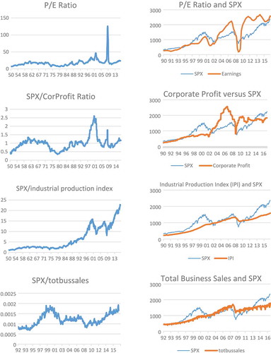
This is the traditional P/E ratio for SPX which has an average of approximately 18 since 1950. The sharp upward spike in 2009 was due primarily to the low level of corporate earnings during the “great recession” (Figure 1). The current P/E ratio is high by historical standards but is not yet at a record level. Based on the 10-year moving average value of the P/E ratio, stocks are near their fair value (see Figure 1).

Figure 1. SPX versus P/E Ratio, Corporate Profit, Industrial Production and Total Business Sales

3.2. SPX/corporate profit (PROFIT)

This ratio relates stock prices to before tax corporate profits as provided by the U.S. Bureau of Economic Analysis. Although this ratio is related to the P/E ratio, it is currently high by historical standards, suggesting that stock prices are currently overvalued (see Figure 1).

3.3. SPX/industrial production index (IPI)

This ratio is currently at its highest point. Stock prices would be expected to grow as industrial production grows. However, the growth in stock prices is significantly greater than the growth in industrial production (see Figure 1). This growth disparity may simply reflect the fact that recent economic growth had come primarily from the service side of the economy.

3.4. SPX/total sales (SALES)

This ratio relates stock prices over time to total business sales. This ratio is currently at its highest point, slightly above its level in 1999. The gap between SPX and fair value has been expanding since 2013 and is currently at its widest, suggesting the stock market is richly valued.

3.5. SPX/bond index ratio (BOND)

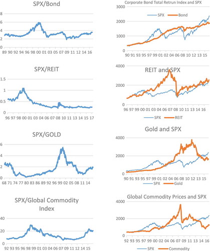
Bonds should provide a useful benchmark since they represent the most direct investment alternative to stocks. The BofA Merrill Lynch US Corp Total Return Index is used to represent the performance of corporate bonds. The SPX/Bond ratio is not particularly high. However, stock prices are relatively high when the historical moving average of the bond index is used to find fair value. More specifically, it appears that stocks were relatively cheaper between 2002 and 2013 and relatively more expensive since then with a growing gap between current market levels and the value suggested by a long-term average of this ratio. (See Figure 2).

Figure 2. SPX versus Bond, REIT, Gold, and Commodity Index

3.6. SPX/REIT ratio

Like bonds, REITs are traditionally viewed as an alternative investment. Indeed, many researchers have found that REIT performance is similar to that of small cap stocks. The SPX/REIT ratio is currently at a relatively low level suggesting that stocks are not currently overpriced. Although REITs have been observed to behave like small cap stocks, this is still and interesting and somewhat unexpected result (see Figure 2).

3.7. SPX/Gold

Many consider gold to be a store of value and a hedge against inflation. Furthermore, gold is an alternative investment and as such represent an important benchmark for stocks. The SPX/Gold price ratio is not currently high. From 2002 until 2014 gold prices were very high and the ratio was low, particularly during the “great recession.” Now, however, stock prices are higher relative to the price of gold.

3.8. SPX/Commodity (COMOD)

Although gold and oil are considered individually, there is merit in looking at commodities in general. SPX/Commodity price ratio is very high at this time although it has yet to reach its 1999 record level. Current stock prices are significantly higher than the fair value suggested by the global commodity index suggesting that the stock market is overvalued (Figure 2).

3.9. SPX/Oil

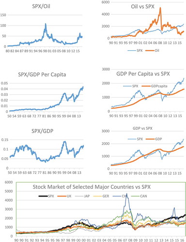
Oil is an important commodity and its price is a factor in the price of most consumed goods. The SPX/Oil price ratio is currently high suggesting that the stock market might be relatively expensive.(Figure 3).

Figure 3. SPX versus Oil, GDP, and Foreign Stocks

3.10. SPX/GDP per capita (GDPCAPITA)

One might expect parallel movement between stock price levels and GDP per capita and/or GDP. The current SPX/GDP per capita ratio represents a historic high. When one compares the actual value of SPX with the fair value of SPX based on GDP per capita, it is apparent that stock prices have grown much faster than GDP per capita. The current high level of the GDP per capita ratio is consistent with a stock market that is overvalued (Figure 3).

3.11. SPX/GDP

Similar to the GDP per capita ratio, this ratio is currently high although not at its highest point. When the current value of SPX is compared with the fair value of SPX based on GDP, the stock market appears to be overpriced (Figure 3).

3.12. SPX/international stock indexes

This ratio relates the US stock values to the average stock market levels of the 20 largest economies in the world and is currently very high. If the stock prices of other countries are used as a benchmark to calculate the fair value of SPX, the current US stock prices are overvalued. US stock market is also high relative to stock market levels in all of the major world economies if compared individually. Relative value of Chinese market has spiked higher than in 1999, 2000, 2007, 2009, and 2015. Currently, the US stocks are relatively expensive compared to those of China and all of the other individual stock markets (Figures 3 and 4).

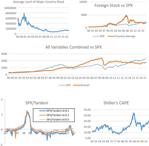
Figure 4. SPX versus Average Foreign Stocks, All Variables, Yardeni, and Shiller's CAPE

3.13. Overall average

Finally, an index is created using the average of all the ratios discussed so far. The current level of this index is at a high level, which is very close to the highest point recorded around years 1999 and 2000.

Two main crossovers can be observed. Before May 2002, the actual value of SPX was higher than the fair value estimate. Between 2002 and 2013, the fair value of stock was higher than SPX including the period just the before mortgage crisis. The second crossover happens at the end of 2013. Since that time, the SPX index is higher than its fair value.

In other words, using some of the most important benchmarks (company related variables, economy-wide variables, bond indexes, alternative investments, and other countries), it is safe to conclude that current stock prices are high (Figure 4).

4. Methodology

Each of the ratios discussed so far in the data section can be considered a fair stock valuation model in itself. However, our objective is to identify models that best explain the data. The Fed model and modified fed model by Yardeni (2003) are the models that aim to find the fair value of stocks.

4.1. Yardeni’s model

Yardeni’s (1999, 2003) model modifies the Fed model¹ by combining it with the Gordon growth model (the model uses earnings rather dividends):

(1) $P_0=\frac{E_1}{r-g}$(1)

where $E_1$ is the expected stock earning for the following year, r is the required rate of return for the stock, and g is the expected long-term growth rate of earnings.

Yardeni uses Moody’s A rated corporate bond yield for r (10-year maturity) (similar to the Fed model) and uses the consensus 5-year growth estimate compiled by Thompson Financial. This growth estimate is called LTEG. Yardeni does not use the raw growth in the model but instead use a weighted LTEG in the formula. Yardeni finds that investors do not put a large weight on the growth estimates (LTEG) since it usually exceeds the actual growth. The typical weight used in Yardeni’s models is 0.1. Therefore, the final version of the model is given as follows:

(2) $P_0=\frac{E_1}{r_{A-rated}-d\times LTEG}$(2)

where d is the weight. Using the Yardeni’s model, a fair value for SPX is calculated. Then the log ratio of actual SPX index value and fair value from the Yardeni’s model is calculated. For example, in August 2016, the earnings estimate for SPX index was $89.09, the long-term earnings growth rate estimate (LTEG) was 10.19%, and A rated corporate bond yield was 4.24%. Given these figures, Yardeni’s model would estimate the value of SPX as 2766, much higher than the actual SPX value of 2171 at the time. The log ratio of SPX value to the value estimated by Yardeni’s model is negative (ln(2171/2766)). The negative ratio suggests that the SPX is relatively cheaper as compared with the value suggested by Yardeni’s model in August 2016.

According to this measure, SPX currently is slightly undervalued (Figure 4). This is true for if the d value is assumed to be higher than 1.6%. However, if the d value is assumed to be less than 1.6%, then SPX is overvalued. The Yardeni’s model recognizes only bonds as an alternative to stocks and benchmarks the stock value to A-rated corporate bonds. A model using the commodities, foreign equity, real estate, and some macroeconomic variables may provide better stock valuation.

4.2. Cyclically adjusted price/earnings ratio (CAPE)

Shiller (2000, 2005, 2015) calculates cyclically adjusted price/earnings ratios of stock prices (CAPE). The real SP-500 index is divided by the past 10-year moving average of real earnings. CAPE level was around 30 in the first half of 2017 which is high by historical standards except for the few years around 2000 (Figure 4). Because the CAPE utilizes the earnings only, the inclusion of other possible benchmarks may provide a more accurate assessment of stock market valuation.

4.3. Alternative stock valuation models

Next, we tested whether all these variables as a group can explain a significant part of the variation in SPX. To develop a successful model, we first looked at the correlations between SPX and all the variables in the data sample. The correlation between SPX and most of these variables are significant and high, which is promising for the development of a successful model. The highest correlation (97%) is between SPX and Swiss stock market index. GDP, earnings, profits, and IPI are also highly correlated with SPX. Oil and commodities in general have low correlation with SPX. This low correlation confirms the importance of oil and commodities in diversifying risk. It is interesting to note that the correlations between US stock market and Swiss, UK, Canada and Australian stock markets are very high while the correlation between US market and those of Spain and Sweden are very low. The foreign stock market indexes were converted to dollars using the exchange rate at the time. The correlation would have been higher if the indexes were in domestic currency (see Table 2).

Table 2. Correlations among Spx and all other variables

BOND	0.89***	AUS	0.88***	NETHER	0.46***
COMOD	0.52***	BRAZ	0.32***	NZEL	0.83***
EARNING	0.94***	CANAD	0.89***	RUS	0.25***
GDP	0.96***	CHIN	0.53***	SAFRICA	0.79***
GDPCAPITA	0.90***	FRANCE	0.51***	SAUDI	0.34
GOLD	0.72***	GERMAN	0.75***	SPAIN	0.10
IPI	0.90***	INDI	0.85***	SWEDEN	0.10
OIL	0.58***	INDO	0.62***	SWISS	0.97***
PROFIT	0.93***	ITALY	−0.07	TUR	0.71***
REIT	0.85***	JAP	0.54***	UK	0.93***
SALES	0.85***	KORE	0.68***	COUNTRY	0.92***
		MEX	0.68***

***, **, * Significant at 1%, 5%, and 10% level, respectively. These are the pairwise correlations between SPX and all the variables listed in the table. The largest correlation is between Swiss Stock Market Index and SPX. GDP, earnings and profit are also highly correlated with SPX. Italy’s stock market index is negatively correlated with SPX. Commodities and oil have low correlation with SPX. These alternative assets could be valuable for diversification.

Using 10-year moving averages of the ratios of SPX to each variable, we calculated a fair value for SPX as it is explained above. A positive difference between SPX and our fair value shows that the stock market is overpriced. Using country averages and all other variables described in the data section, the overall fair value and the difference between the fair value and SPX is calculated for each month. We created a dummy variable that takes a value of 1 if the SPX is greater than the fair value at a given month. The value of the dummy variable would be 0 if the fair value is greater than the value of SPX.

To explain how this process works, assume that only two variables are used as benchmark instead of 12 variables actually used in the study. On 31 January 2017, the value of SPX was 2278.87; the IPI 103.5; and gold prices were 1203. Ten-year moving average of SPX/IPI was 15.06 and SPX/GOLD was 1.34 at the same date. So justified SPX levels using the 10-year averages of these two variables can be computed. This number using IPI is (15.06*103.5) 1558.71. The justified level of SPX using GOLD is 1612.02 (1.34*1203). Now let’s average these two numbers (in the paper we would have 12 such numbers and we would average 12 numbers to find the fair value of the SPX for that month). The average is 1585. This number is the fair value we computed for SPX. The actual SPX for that month was 2278.87. The value of SPX is greater than the fair value we computed using all the variables we used. Thus, for that month the dummy variable will take a value of 1. Had SPX value been smaller than the computed fair, the dummy variable would have taken a value of zero. In a regression, the coefficient of the dummy variable should be positive since there is a greater chance that SPX is overpriced as it is level gets relatively higher.

Finding a good regression model is important. A good model should be simple but powerful and econometrically sound. In this section, you will find the process of finding this model. A reader who would like skip this discussion and want to see the final model, can look at the model in Equation 5 directly.

First, we used a regression model without a dummy variable. We used all countries individually and all other variables and used stepwise selection method to decide which variables to include in the regression:

(3) $SP{X}_t=a+b{B}_t+c{C}_t+d{R}_t+e^{\prime }{E}_t+F^{\prime }M+{\epsilon }_t$(3)

where SPX is the Standard and Poors’ 500 index, B_t is the bond index, C_t is the commodity index, R_t is REIT index, e′ is the vector of coefficients of foreign stock exchanges, E_t is the vector of foreign stock indexes, F is the coefficient vector of macro-economic variables, and M is the vector of the macro-economic variables. The results are presented in Table 3.

Table 3. Various regression models

Equation (3)		Equation (5)		Equation (6)
Variable	Coefficient	Variable	Coefficient	Variable	Coefficient
SWISS	950.1433	BOND	1.421976	C	−785.8227
SAFRICA	−2658.898	DUM	387.8779	FAIR	1.171751
OIL	4.281692	COMOD	−0.496559	DUM	850.3824
BOND	1.144757	C	−2255.804	GOLD	−0.081035
NETHER	555.0292	IPI	29.87364
SWEDEN	−507.9976
COMOD	−5.829598
CANAD	610.2987
R^2	0.972134		0.959721		0.690223
Adjusted R^2	0.971209		0.959160		0.686318
Included observations	219		292		242
Number of search regressor	33		_		_

All coefficients are significant at 1% precision level. The only exception is COMOD and GOLD. These two variables are not significant.

Not surprisingly, most of the variables are significant² and the R² is very high (97%). Swiss, South African, Dutch, Sweden, and Canadian stock market indexes are significant in the equation. Oil, bond and commodities are other significant variables. In this format, the model is somewhat complex and have serious multicollinearity. To simplify the model, the foreign stock indexes were excluded. R² in this model is a bit lower (96%) compared to previous model but the model is much simpler. This result suggests that, further models should use an average of the indexes for all foreign countries rather than using separate indexes for each country. Next the dummy variable is added to the regression model:

(4) $SP{X}_t=a+b{B}_t+c{C}_t+d{R}_t+e{E}_t+F^{\prime }M+g{D}_t+{\epsilon }_t$(4)

where D is the dummy variable we created using our moving average fair value and E is the country index created with averaging all country indexes. When the dummy variable is added to this regression, the R² now improves to the point that this model has the potential to explain 97% of the variation in SPX. In this second regression model Bonds, the dummy variable, earnings, commodities, country indexes and IPI were the significant variables. All coefficients are positive except the coefficient of commodities. This result suggests that commodities could be invaluable in portfolio diversification. After further tests, we had to remove the variable COUNTRY and EARNING to correct the multicollinearity problem in the regression. All the variables used in this regression have unit roots. The first difference of each variable is stationary. The regression model with the differenced variables can only explain 27% of the variation in differenced SPX. On the other hand, we found some cointegration equations among variables SPX, COMOD, COUNTRY, EARNING, IPI, GOLD, and SALES. Therefore, canonical cointegrating regression is used to solve the spurious regression problem. The resulting model can explain almost 96% of the variation in SPX:

(5) $SP{X}_t=a+b{B}_t+c{C}_t+e{I}_t+g{D}_t+{\epsilon }_t$(5)

where B_t is bond index, C_t is commodity index, I_t is the IPI, and D_t is the dummy variable.

Removing COUNTRY and EARNING did not have a significant impact on the model.

Is it possible to further simplify the model by using fewer variable?

(6) $SP{X}_t=a+bFai{r}_t+c{L}_t+d{D}_t+{\epsilon }_t$(6)

where L is the GOLD prices. This is the only model with the fewest variables and still have stationary residuals. Using the fair value created using the average of all the variables, gold prices, and the dummy variable, it is possible to explain 68% of the variations in stock market.

If the dummy variable is removed from this model, then R² decreases significantly. It is possible to simply the regression at a cost of significantly decreasing R². Regression as defined in Equation 5 has only four variables and can explain up to 96% of the variation in SPX. Therefore, we will use this regression in the next section.

This section is quite lengthy. However, we include all this discussion to show how we arrived to the model in Equation 5 with only four variables. This section starts with 33 variables. Removing 29 variables simplify the model significantly; solves most of the econometric problems associated with the regression model; and the cost of removing 29 variables is not significant.

4.4. Duration dependence test

To the extent that fundamentals do not support the current levels of stock prices, one possible explanation is rational bubble. A rational bubble exists if market participants realize that the prices are higher than the level supported by the fundamentals but continue to hold the stocks with a firm belief that market prices will go higher. This section will analyze whether the current stock market level represents such a bubble by using the approach taken by McQueen and Thorley (1994). McQueen and Thorley (1994) assert that a rational bubble exists if the probability of a crash after a series of positive abnormal returns declines as the number of consecutive positive abnormal returns increases.

Using the residuals from regression model defined by Equation 5, we created an abnormal return series. The factors used in Equation 5 explain almost 96% of the variation in SPX and the residuals from this regression should be random and have an expected value of zero. There should be no pattern to the abnormal returns. If consecutive abnormal returns are all positive, this suggests a possible bubble in stock market prices. This section will closely analyze the abnormal returns to determine whether or not this is the case. A series of consecutive positive or negative abnormal returns is considered to be a run. A series of 10 consecutive positive abnormal returns followed by a negative abnormal return represents a positive run with a length of 10. When consecutive positive returns are followed by a negative return or vice versa, a run ends. All returns are classified into positive and negative runs with a run length are calculated for each. If the abnormal returns are random, then the probability of a long positive or negative run should be extremely low.

Suppose X_t is the abnormal return of SPX in the month of t. A positive run with a length of L can be defined as follows:

(7) $R_L\in \left\{X_t⟨0|X_{t-1}>0,\dots ,X_{t-l}>0,X_{t-L-1}<0\right\}\mathrm{\forall }t\le nandL\le t$(7)

where n is the number of total returns in the sample. The hazard rate (h_t) is the probability that the bubble will burst in the next period given the lag length:

(8) $h_t=\frac{1}{1+e^{-d_t}}$(8)

where $h_t$ is the probability that the run will end, and

(9) $d_t=\alpha +\beta LnL$(9)

The parameters are estimated with a logistic regression. The dependent variable is whether the run ends or not (1 or 0), and the main independent variable is the lag length (L). The likelihood ratio test is used to test the significance of $\beta$, which is asymptotically a chi-square distribution with one degree of freedom.

If there is a bubble, the hazard rate should decrease as the lag length increase. In other words, the longer the bubble, the less likely it would burst in the next period. Suppose there is a positive run with the lag length of 5. That is, there are five consecutive positive abnormal returns. The probability that the bubble may burst in the next month is about 6.85% assuming both alpha and beta are −1 for simplicity using the Equations 8 and 9. Now, suppose the run length is 20 instead. The probability of bubble bursting during the next month would be only 1.81%. If this test is done and the estimated coefficient of beta is negative and significant, then this would be evidence of a bubble as described above. If we cannot reject that the probability of bubble bursting is the same regardless of the lag length and whether the run is positive or negative then there is no evidence of a rational bubble.

Using the monthly abnormal returns (residuals) from the regression as defined in Equation 5, parameters of Equations 8 and 9 are estimated (see Table 4 for the results).

Table 4. Run counts and duration dependence test

Run Length	Positive runs	Negative runs
1	9	5
2	3	3
3	3	3
4	0	1
5	0	1
6	1	2
7	0	0
8	0	2
9	1	0
10	1	1
11	1	0
12	0	0
13	1	2
14	1	0
24	0	1
26	1	0
Log-logistic test
Alpha (α)	−0.61	−1.25***
Beta ($\beta$)	−0.62**	−0.2
LRT of $H_1:\beta =0$	6.21	0.56
p-value	0.01	0.45

Runs are consecutive positive and negative abnormal returns derived from the residuals from the regression model 4. ***, **, and * Significance of each coefficient at 1%, 5%, and 10% level, respectively. Alpha is the coefficient of the constant and beta is the coefficient of log run length. Log-likelihood test (LRT) tests the significance of beta. The restricted model assumes that the beta is zero. That is, there is no relationship between run length and probability of a market crash. The test is a chi-square test with one degree of freedom. The significantly negative beta coefficient for the positive runs indicates that there is an evidence for a rational bubble in the stock market. Negative coefficient suggests that as the run length increases, the probability of crash decreases.

It is normal to see the largest number of runs would have a run length of 1 and 2. There are nine positive runs and five negative runs with run length of one. Furthermore, one would expect numbers of a particular length to decrease as the run length increases. We observed one positive run with a length of 26 months, which is highly unlikely as a random event. Imagine trying to flip a fair coin to get 26 heads in a row. Beta is negative and significant for positive runs but not significant for negative runs. The conclusion we can draw is that a rational bubble is an explanation for positive runs but not for negative runs. Based on the parameters from the Table 4, the probability that bubble may burst in the next month with a current run length of 5 is 17%. If the run length is 26, the same probability is 6.7%. This represents strong evidence of a rational bubble which, in turn, represents the only clear justification for the current level of stock prices.

5. Conclusions

This paper uses bonds, commodities, REITS, gold, oil, company earnings, sales, industrial production, GDP, and other country’s stock markets as benchmarks to judge the current level of SPX. According to all these measures, except for earnings, the stock market is overpriced. All of these measures suggest that the current level of the stock market is high. The only other time relative stock prices were this high was immediately before the crash of tech bubble in 2000. This paper also offers an alternative benchmark for the stock market, which can explain 96% of the variation in SPX. Although fundamentals do not support the current level of the market, a rational bubble may. Strong evidence of a rational bubble is found in the returns of SPX. All of this suggests that investors would be wise to carefully limit their exposure to U.S. stocks.

Additional information

Funding

The authors received no direct funding for this research.

Notes on contributors

Riza Emekter

Riza Emekter is a professor of finance at Robert Morris University. He mainly teaches investment courses. He has published more than 15 articles in scholarly journals in various investment related topics. His current main research interests are in asset allocation and portfolio optimization.

Robert Beaves

Robert Beaves is a professor of finance at Robert Morris University. He has a PhD in finance and a JD from the University of Iowa. He is a registered investment advisor representative and holds the CFP designation. He has taught investment classes for over 40 years.

Zane Dennick-Ream

Zane Dennick-Ream is an assistant professor of finance at Robert Morris University. His academic training is in finance, applied economics, and mathematics. His main research interest is in corporate finance.

Notes

1. Fed model is a simple equity valuation models which asserts that expected stock earnings yield is equal to 10-year treasury bond yield ($\frac{E_1}{P_0}=r_{10}$) This model was popularized by Yardeni. See Yardeni (1999) for more details.

2. Since stepwise regression is used, it is natural that significant variables would filter through in this process and most of the insignificant variables (not all) will be left out.

References

- Balke, N. S., & Wohar, M. E. (2001). Explaining stock price movements: Is there a case for fundamentals?. Economic & Financial Review-Federal Reserve Bank of Dallas, (3), 22–33.
- Barker, R. G. (1999). Survey and market‐based evidence of industry‐dependence in analysts’ preferences between the dividend yield and price‐earnings ratio valuation models. Journal of Business Finance & Accounting, 26(3‐4), 393–418. doi:10.1111/1468-5957.00261
- Barsky, R. B., & De Long, J. B. (1990). Bull and bear markets in the twentieth century. The Journal of Economic History, 50(2), 265–281. doi:10.1017/S0022050700036421
- Campbell, J. Y., & Shiller, R. J. (1988). Stock prices, earnings, and expected dividends. The Journal of Finance, 43(3), 661–676. doi:10.1111/j.1540-6261.1988.tb04598.x
- Campbell, J. Y., & Shiller, R. J. (2001). Valuation ratios and the long-run stock market outlook: An update (No. w8221). National bureau of economic research.
- Carlson, J. B., Pelz, E. A., & Wohar, M. E. (2002). Will valuation ratios revert to historical means? The Journal of Portfolio Management, 28(4), 23–35. doi:10.3905/jpm.2002.319851
- Carlson, J. B., & Sargent, K. H. (1997). The recent ascent of stock prices: Can it be explained by earnings growth or other fundamentals? Economic Review-Federal Reserve Bank of Cleveland, 33(2), 2.
- Coakley, J., & Fuertes, A. M. (2006). Valuation ratios and price deviations from fundamentals. Journal of Banking & Finance, 30(8), 2325–2346. doi:10.1016/j.jbankfin.2005.08.004
- Cochrane, J. H. (1998). Where is the market going? Uncertain facts and novel theories (No. w6207). National Bureau of Economic Research.
- He, L. T. (2009). What can we learn from 123 years of stock market fluctuations? Processes of mean aversion and reversion. The Journal of Investing, 18(4), 57–71. doi:10.3905/JOI.2009.18.4.057
- Heaton, J., & Lucas, D. (1999). Stock prices and fundamentals. NBER Macroeconomics Annual, 14, 213–242. doi:10.1086/654387
- Manzan, S. (2007). Nonlinear mean reversion in stock prices. Quantitative and Qualitative Analysis in Social Sciences, 1(3), 1–20.
- McMillan, D. G. (2009). Are UK share prices too high? Fundamental value or new era. Bulletin of Economic Research, 61(1), 1–20. doi:10.1111/boer.2008.61.issue-1
- McQueen, G., & Thorley, S. (1994). Bubbles, stock returns, and duration dependence. Journal of Financial and Quantitative Analysis, 29(3), 379–401. doi:10.230723/31336
- Nasseh, A., & Strauss, J. (2000). Stock prices and domestic and international macroeconomic activity: A cointegration approach. The Quarterly Review of Economics and Finance, 40(2), 229–245. doi:10.1016/S1062-9769(99)00054-X
- Phillips, P. C., Wu, Y., & Yu, J. (2011). Explosive behavior in the 1990s Nasdaq: When did exuberance escalate asset values? International Economic Review, 52(1), 201–226. doi:10.1111/j.1468-2354.2010.00625.x
- Shiller, R. J. (2000, 2005, 2015). Irrational exuberance. Princeton university press.
- Yardeni, E. (1999). New, improved stock valuation model. Topical Study, 44. Retrieved from http://www.yardeni.com/pub/t_990726.pdf
- Yardeni, E. (2003). Stock valuation models (4.1). Topical Study, 58. Retrieved from http://www.yardeni.com/pub/t_080802.pdf