Accuracy, unbiasedness, and efficiency of current account growth forecast: Evidence from a large cross section of developed and developing economies

Abstract

We use a previously unexploited consensus survey data set to compare accuracy, unbiasedness and efficiency of Current Account growth forecasts between two panels of 25 developed and 18 developing countries following the methodologies in the existing literature. Forecast errors are bigger for the developing country comparing to the developed country. Developed country forecast errors are unbiased but inefficient. The developing country forecast errors are biased but relatively more efficient. In both the panels, forecast revisions are efficient for the same forecast horizons, but inefficient for the adjacent horizons. Additionally, we find less evidence of forecast smoothing compared to some earlier studies. Forecasters do improve their forecasts as the horizons become shorter although the forecasts fall short of being unbiased and efficient statistically.

Keywords:

• forecast efficiency
• panel estimation
• consensus survey
• developing economies
• rational expectations

JEL classification:

• E27
• E37; E00

PUBLIC INTEREST STATEMENT

Professional forecasts of Current Account growth rates are inefficient meaning forecasters do not incorporate all available information in their forecasts. Forecasters do reduce forecast errors continuously over time by incorporating new information as they become available. Forecasting of developing country is more efficient than the developed country. Economic agents should use these data carefully. Policy makers should release more information so as to make forecasting better.

1. Introduction

Forecasting of key macroeconomic variables has become an important trend in many business and government organizations in the recent past as economic agents use them in making important economic and financial decisions. While many large businesses and government agencies create their own forecasts in-house, many others purchase them from outside vendors. One particular type of forecast known as consensus survey forecast¹ have drawn considerable interest among professionals and academicians. Academicians attempt to understand the accuracy of these forecasts² as these are opinions of experts not general public. The central question that researchers try to investigate is whether these forecasts correctly predict the future.

Many studies examine unbiasedness and efficiency³ of several economic variables, including exchange rates, interest rates, inflation rates, GDP growth rates, industrial production rate, unemployment rate, commodity prices, etc. using consensus survey data from various sources. However, there are limited sources of these data. Pesaran and Weale (2006) and Stekler (2002) list major sources of survey data and present summaries of the most commonly used approaches in testing forecast efficiency. General conclusion of these studies reveals that survey forecasts are biased both at the individual and at the average level. Nordhaus (1987) argues that the bias could be due to model formulation, estimation, or simulation problems. He also argues that the forecasters themselves could even generate the bias on purpose due to fear of loss of reputation (meaning too slow to utilize new information). Some researchers have shown that forecasters over-react to new information (Ashiya, 2002, 2003; Clements, 1995, 1997; Ehrbeck & Waldmann, 1996) while others have found that analysts under-react to new information (Amir and Ganzach, 1998; Abarbanell & Bernard, 1992; Chen, Costantini, & Deschamps, 2016). In the context of macroeconomic forecast, most of the available studies examine the developed economies more than the developing economies. Few studies show some differences in the results between the developed and the developing economies (Chen et al., 2016; Loungani, 2001; Loungani, Stekler, & Tamirisa, 2013). The latter two studies use data from the same source. Therefore, there is a need for further study on the unbiasedness and efficiency of expectations of these important macroeconomic variables using new data sources, especially for the developing economies. This paper attempts to extend the limited work on the issue by studying forecast accuracy, unbiasedness and efficiency of Current Account (CA) growth rates⁴ of 25 developed and 18 developing countries, using a previously unexploited consensus survey data set. The study highlights the differences in the results between the developed and the developing countries as two separate panels. Additionally, although there are many studies on macroeconomic variables, there is no study on the unbiasedness and efficiency of CA growth rate. CA is an important macroeconomic variable to both policy makers and financial market participants as it impacts GDP, currency exchange rates and other macroeconomic variables. It is an important channel though which external shocks permeates an economy. The results of this study will enhance our understanding of forecast efficiency in general, especially for the developing countries, which will be useful to both researchers and policy makers.

In short, this paper attempts to answer the following questions:

1. Are the forecasts of CA growth rates unbiased and efficient?

2. Are the forecast revisions of CA growth rates efficient?

3. Do the forecasters learn from their mistakes? Do the forecasts improve over time?

4. Is there evidence of forecast smoothing as suggested by some earlier studies?

5. Are there significant differences in the results between the developed and the developing country panels?

The rest of the paper is organized as follows. Section 2 provides a brief literature review of the area. Sections 3 and 4 discuss the methodology and the data used for empirical investigation. Section 5 reports, analyzes, and compares the results. Finally, Section 6 concludes the paper.

2. Literature review

Many studies have analyzed the accuracy, unbiasedness and efficiency of forecasts in the recent past using survey data. Some studies examine performance of an individual forecaster or organization while others examine the efficiency of average forecast of an expert panel (consensus forecast). Forecasts of a number of economic and financial variables are examined in these studies. Some studies investigate the unbiasedness and efficiency of forecast revisions while others investigate the unbiasedness of forecast itself. The fixed event nature of the forecasts of our data set enables us to examine efficiency of forecast error as well as the revision.⁵ Most studies find that forecast errors and revisions are biased in general. However, some country specific investigations find less evidence of biasedness. Some studies investigate the developed and the developing countries as two separate groups and find different results between the two groups. We summarize a few recent studies including the original first study by Nordhaus (1987) focusing on those studies that closely relate to our type of data and variables of interest (see Table 1).

The above studies clearly show that most macroeconomic forecasts are biased and inefficient in general, but there are exceptions as well. We also note that most studies focus on the biasedness and efficiency of GDP and inflation rates as these are the two most important macroeconomic variables policy makers and other economic agents are concerned with. Thus, there is a room for investigation of unbiasedness and efficiency of forecasts of other macroeconomic variables, like CA growth rate, using different survey data sources. CA is an important macroeconomic variable for many countries as it directly affects exchange rates and GDP. Thus, it should also be investigated.

Unbiasedness and efficiency hypothesis has been tested widely using exchange rate and interest rate data as well. The most recent survey of literature in these areas is available in Miah, et al. (2016), Jongen, Verschoor and Wolf (2008), and Jongen and Verschoor (2007). The general conclusion of these studies reveal that survey data is a biased predictor of future change in interest rates, exchange rates, and that agents do not incorporate all available information in forming their expectations.

3. Research methodology

Following Ashiya (2006), we define the survey-based forecast error, FE_−i,t, as the difference between the forecast, F_−i,_t which is the forecast for year t released i months prior to the end of year t, and the actual realization, A_t, which occurs at the end of year t. In notation, FE_−i,t, = F_−i,_t—A_t, where i = 1, 2, 3, 4 … 24 are forecast horizons. Similarly, we define forecast revision, FR_−i,t, as the forecast revision that was made in months prior to the end of year t. In notation, it is FR_−i,t, = F_−i,_t—F_−i-1,_t. Note that there are 24 monthly forecasts for each year, but one actual realization at the end of year t. In other words, forecast for a particular year starts 2 years early and continues for 24 months. Because of some missing data, we omit the last month (horizon 24) from the analysis. Thus, we have 23 horizons.

3.1. Accuracy of forecasts

Following Bowles et al. (2007) and Loungani (2001), we calculate mean error (ME), mean absolute error (MAE), root mean square error (RMSE), and Theil’s inequality coefficient (TIC) to measure forecast accuracy. ME is the average difference between the forecast value and the actual realized value. If the forecasts are unbiased and shocks are symmetric, then the ME should be zero on average. MAE is the absolute value of the differences between the actual and the forecast values averaged across all countries and overall years. It provides information about the average size of forecast errors, whether they are positive or negative. RMSE is the root of the forecast errors squared and averaged over the sample. TIC is another alternative measure, which is RMSE divided by the variability of the underlying data. It is used to understand if a forecast performs better than a naive forecast of no change in the growth rate between two successive periods. TICs of less than one for a forecast are considered better than the naive forecast. Each of these measures is a successive improvement of shortcomings in the previous measure.⁶

3.2. Unbiasedness and efficiency of forecast errors

Unbiasedness of forecasts means that forecasts should be approximately equal to the realized value on average over time, and thus, forecast errors will be approximately zero on average over time. On the other hand, efficient forecast requires that the forecasts should come from accurate models of economic behavior that use all relevant information publicly available at the time of forecast. Forecasts cannot be further improved by using any other model or readily available information.

First, we examine unbiasedness and efficiency of forecast errors by performing the following regression:

(1) $F{E}_{-i,t}=a+bF{R}_{-i,t}+e_{-i,t}$(1)

Unbiasedness requires that a = 0 and efficiency requires that b = 0 in the above equation. An acceptance of a = 0, indicates that the forecast is unbiased.⁷ An acceptance of b = 0 indicates that forecasters use all available information at the time of forecast efficiently in their forecast revisions. If a forecast is efficient, its forecast error should be independent of its past forecast revisions. Nordhaus (1987), Ehrbeck and Waldmann (1996), Amir and Ganzach (1998), Ashiya (2006) considered the above regression.

3.3. Efficiency of forecast revisions

Then, we examine the efficiency of forecast revisions by performing the following two regressions as considered by Berger and Krane (1985) and Ashiya (2006). Nordhaus (1987), Clements (1995) and Loungani (2001):

(2) $F{R}_{-i,t}=a+bF{R}_{-i,t-1}+e_{-i,t}$(2)

(3) $F{R}_{-i,t}=a+bF{R}_{-i-1,t}+e_{-i,t}$(3)

The null hypothesis of efficiency is that b = 0 in both the equations. In other words, if a forecast revision is efficient, it should be uncorrelated with any past or future revisions. The idea is that if forecasts are formed consistently, then current forecast revisions should not be at all predictable from past revisions.⁸ We allow a nonzero intercept term in the regression equations to accommodate shocks in the economy. An economy can experience continuous shocks in either direction for an unknown period. Equation 2 evaluates serial correlation of forecast revisions for a fixed forecast horizon. This equation correlates one year early forecast revisions with the one year later revisions. For example, say, forecast revision of horizon 5 last year and forecast revision of horizon 5 this year, and so on. Acceptance of the null hypothesis indicates that the forecasters effectively utilize all available information previously used to revise the forecast for the same horizon. Equation 3 evaluates the serial correlation of forecast revisions for a fixed future realization. For example, say, forecast revision of the last month with the revisions of the month before, and so on. An acceptance of the null hypothesis confirms that the forecasters successfully utilize the information previously used to revise the forecast for the same year-end realization.⁹ If b is greater than 0, it indicates that a forecast revision in one direction tends to be followed by further revisions in the same direction. This is described as forecast smoothing in the literature and it is a sign of forecast inefficiency.

We use the panel method to estimate all our equations because our data includes both cross section and time series. Since the data is pooled across countries and over time, there are valid reasons to suspect that our error term would not be random. Therefore, our inferences could be biased. We control for these possibilities by allowing fixed effects in the regression equations across both the cross section and the time dimensions. The idea is that some years may be easier to forecast than some other years for all countries. Similarly, some countries may be harder to forecast than some other countries for all years. The fixed effects will pick up these differences.¹⁰

We have 16 actual yearly realizations of CA growth rates for 43 countries. However, as we mentioned earlier that there are 24 monthly forecasts for each target year. We consider them as 24 forecast horizons. We pool the data across countries and across time by each horizon rather than by each target year. Thus, we have one regression for each horizon. For example, for horizon 5 regression, we have 16 actual annual data and 16 forecasts at horizon 5, one for each target year. We poll the countries together in the panel. We divide the countries into two panels: developed and developing. Twenty-five countries are classified as developed and the remaining 18 are classified as developing following United Nations (UN) country classification system.¹¹ We compare the results of the two panels—developed and developing country in the paper.¹²

4. Data description

We collected survey data from www.fx4casts.com. They are a leading provider of survey data on currency and some key macroeconomic variables. We have actual yearly CA growth rates data for 43 countries from 11/2001 to 12/2016. Several features of the data set are worth mentioning. First, FX4casts.com collects data from a group of experts every month, and the pool of the experts is kept unchanged. Second, FX4casts.com uses geometric mean when computing aggregate consensus forecasts. By exponentially reducing the weight given to extreme forecasts, this reflects more accurately the contributors’ predominant expectations. Third, the survey starts two years early. For example, the forecast for 2010 year-end CA growth rate will start in January of 2008. Therefore, there are 24 forecasts for each target year for each country. Thus, we consider these forecasts as a fixed event forecast. Fourth, the survey data is collected during the third week of each month and is published monthly.

5. Empirical results

5.1. Forecast accuracy

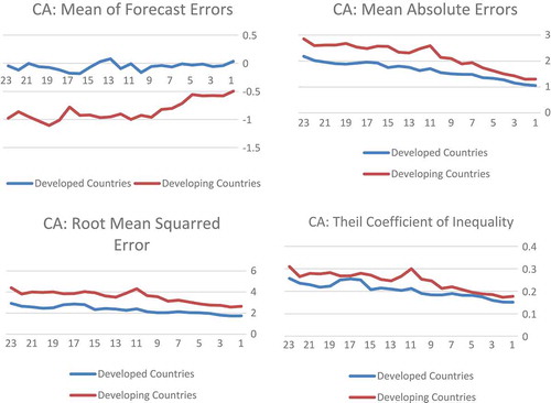
We report four measures of forecast accuracy. These are ME, MAE, RMSE, and TIC as discussed in the methodology section. We compare these statistics between the developed and the developing countries as two groups across both the variables.

Several findings emerge when these measures are taken together. First, the magnitude of the forecast error declines as the forecast horizons get closer to the actual realization. The mean of forecast error is small and remains close to zero for the developed country, but it is bigger and remains negative for the developing country panel throughout the forecast horizons. Second, absolute errors and root mean squared errors are larger for the developing country panel. Third, TICs are lower for the developed country panel indicating that the underlying variability in the forecast is higher for the developed country. TICs are less than one for both the panels indicating that forecasting procedure is better than a naïve forecast as theory suggests.

5.2. Regression results

Formal test results of Equation 1 are reported in Table 2. As we discussed in the methodology section that an acceptance of the null hypothesis of a = 0 indicates that the forecast errors are unbiased.¹³ The null of a = 0 is accepted in all 23 cases for the developed country, but it is rejected in all 23 cases for the developing country panel. In other words, forecast errors are unbiased across all the horizons for the developed country, but biased across all the horizons for the developing country.

Table 1. Summary of recent studies

Study and period	Objective	Findings	Data source
Ager, Kappler, and Osterloh (2009)/1996–2006	Unbiasedness and information efficiency of average forecast of GDP and inflation of 12 industrial countries	Biased beyond 12-month horizon for all countries. Mixed results for below 12-month horizon. No informational efficiency.	Consensus Economics
Ashiya (2006)/1963–2003	Rationality of forecast revisions of G7 countries Real GDP and GDP deflator made by IMF and the OECD	60% of real GDP and 37% of GDP deflator forecasts are rational.	IMF and OECD
Bakshi and Yates (1998)/1994 −2000	Efficiency of Forecast Error and Forecast Revisions of UK Inflation	Forecasts are biased in general, but efficiency in forecast is not completely ruled out.	Merrill Lynch Consensus Survey
Batchelor (2007)/1990–2005	Unbiasedness and Efficiency of average and individual forecasts of Real GDP and Inflation rates of G7 countries	Average and individual forecasts are Biased and inefficient	Consensus Economics
Boero, Smith, and Wallis (2008)/1996–2005	Average and Individual forecast performance of UK Inflation and GDP growth rates	Unbiased and efficient in general	Bank of England
Bowles et al. (2007)/ 1999–2006	Performance of professional forecasts of GDP, inflation, unemployment rates of Euro area	Bias in individual and average forecasts	ECB professional survey
Chen et al. (2016)/1995–2015	Individual forecast of GDP and Inflation of 10 Asian countries	Bias in general	Consensus Economics
Dovern and Weisser (2011)/ 1991–2005	Individual forecasters performance of annual GDP growth rate, Inflation rate, private consumption expenditure and industrial production of G7 countries	Mixed results by variable, country and individual forecaster	Consensus Economics
Gallo, Granger, and Jeon (2002)/1993–96	Evolution of macroeconomic forecasts of GDP, Industrial production and Corporate profit of US, UK and Japan	Biased individual forecast behavior	Consensus Economics
Harvey, Leybourne, and Newbold (2001)/1990–1997	Individual forecasters performance of UK GDP growth rate, inflation rate, and unemployment rate	Consensus forecast are not optimal	Consensus Economics
Isikler, Lahiri, and Loungani (2006)/1989–2004	Forecast efficiency and degree of inefficiency using average data of Real GDP growth rate of 18 industrial countries	Forecasts are not efficient	Consensus Economics
Loungani (2001)/1989–98	Unbiasedness and efficiency of average forecast of GDP growth rate of 63 Developed and Developing countries	Biased and inefficient with some differences between the two groups	Consensus Economics
Nordhaus (1987)/1978–86	Efficiency of Forecast Errors and Forecast Revisions of Oil prices, Nuclear capacity, Energy consumption, Real GNP. Various countries	Forecast revisions are inefficient	DRI Inc., OECD, Eggers Consensus, UCLA, Wharton, Chase
Timmerman (2007)/1990–2003	Compare Performance of WEO forecast to Consensus Economics of GDP growth and inflation rates of 178 countries	WEO forecasts are biased in general. Performance of WEO and Consensus Economics are similar	World Economic Outlook and Consensus Economics
Schuh (2001)	Unbiasedness and efficiency of US real GDP growth rate, inflation rate, unemployment rate, nominal and real short-term interest rates	Forecasts are unbiased but inefficient in general. Individual forecasters are biased and inconsistent.	Survey of Professional forecast (SPF), Wall Street Journal, Blue chip Economic Indicator.

Table 2. Unbiasedness and efficiency of forecast errors (Equation 1). $F{E}_{-i,t}=a+bF{R}_{-i,t}+e_{-i,t}$

		Developed				Developing
Horizon	Coef.	Value	Std. error	t-Prob.	F-Prob. a = 0, b = 0	Value	Std. error	t-Prob.	F-Prob. a = 0, b = 0
1	a	0.015	0.088	0.867	0.000	−0.540	0.154	0.001	0.001
	b	0.386	0.101	0.000		0.518	0.164	0.002
2	a	−0.029	0.085	0.733	0.001	−0.580	0.147	0.000	0.014
	b	0.261	0.065	0.000		−0.020	0.181	0.913
3	a	−0.048	0.090	0.594	0.017	−0.586	0.151	0.000	0.001
	b	0.168	0.079	0.035		0.471	0.152	0.002
4	a	−0.009	0.099	0.925	0.017	−0.576	0.157	0.000	0.006
	b	0.112	0.188	0.553		0.123	0.186	0.510
5	a	−0.016	0.100	0.877		−0.600	0.164	0.000
	b	0.447	0.123	0.000	0.001	0.282	0.144	0.051	0.002
6	a	−0.022	0.101	0.828		−0.734	0.171	0.000
	b	0.348	0.090	0.000	0.001	0.229	0.164	0.164	0.001
7	a	−0.045	0.104	0.662		−0.817	0.172	0.000
	b	0.699	0.126	0.000	0.000	0.780	0.187	0.000	0.000
8	a	−0.052	0.102	0.609		−0.841	0.172	0.000
	b	0.695	0.167	0.000	0.005	0.142	0.101	0.161	0.000
9	a	−0.083	0.103	0.418		−0.949	0.194	0.000
	b	0.240	0.124	0.053	0.008	0.340	0.151	0.025	0.000
10	a	−0.132	0.107	0.217		−0.927	0.202	0.000
	b	0.204	0.076	0.008	0.014	0.005	0.092	0.957	0.000
11	a	−0.067	0.109	0.542		−0.929	0.215	0.000
	b	0.670	0.072	0.000	0.000	0.722	0.083	0.000	0.000
12	a	−0.025	0.115	0.827		−0.944	0.199	0.000
	b	0.414	0.088	0.000	0.000	0.934	0.107	0.000	0.000
13	a	0.062	0.120	0.606		−0.956	0.198	0.000
	b	0.332	0.129	0.010	0.000	0.215	0.163	0.188	0.000
14	a	−0.035	0.117	0.763		−0.966	0.208	0.000
	b	0.659	0.095	0.000	0.000	−0.002	0.145	0.988	0.003
15	a	−0.070	0.119	0.557		−0.922	0.229	0.000
	b	0.011	0.081	0.895	0.002	0.253	0.191	0.188	0.004
16	a	−0.182	0.144	0.209		−0.798	0.225	0.001
	b	0.255	0.206	0.216	0.007	0.875	0.169	0.000	0.000
17	a	−0.130	0.144	0.366		−0.921	0.218	0.000
	b	0.776	0.188	0.000	0.000	0.608	0.149	0.000	0.000
18	a	−0.084	0.126	0.507		−1.036	0.218	0.000
	b	0.792	0.082	0.000	0.000	0.249	0.160	0.122	0.001
19	a	−0.068	0.125	0.586		−1.065	0.225	0.000
	b	0.517	0.145	0.000	0.000	0.538	0.209	0.011	0.000
20	a	−0.047	0.127	0.713		−1.006	0.227	0.000
	b	0.262	0.129	0.043	0.006	0.285	0.216	0.188	0.001
21	a	−0.049	0.131	0.705		−0.873	0.219	0.000
	b	0.390	0.108	0.000	0.000	0.883	0.164	0.000	0.000
22	a	−0.107	0.136	0.430		−0.862	0.219	0.000
	b	0.184	0.091	0.043	0.003	−0.006	0.111	0.959	0.001
23	a	−0.120	0.128	0.347		−0.534	0.218	0.015
	b	0.779	0.068	0.000	0.000	0.830	0.085	0.000	0.000

Now, we look at the significance of b = 0. As we discussed in the methodology section, an acceptance of the null hypothesis of b = 0 indicates that the forecasters use all available information efficiently in their forecasts. We accept the null of b = 0 in only 2 cases for the developed country, and accept it in 11 cases for the developing country. Therefore, forecasts are inefficient for the developed country. But we have mixed results for the developing country. We conclude that forecasters are better able to incorporate information in their forecasts for the developing country than the developed country. Taken together, the results indicate that developed country forecasts are unbiased but inefficient. The developing country forecasts are biased but relatively more efficient as the efficiency test holds true in about 50% of the horizons. We also report the results of the joint null of a = 0, b = 0, and the results show a clear rejection of the joint null across all the horizons in both the panels.

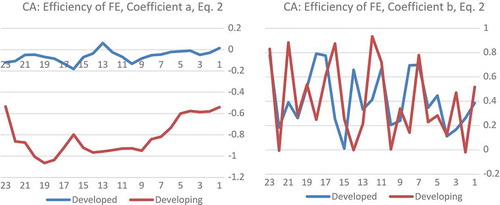
Now we closely look at the trends of these coefficients individually across the horizons and the panels as shown in Graph 2. We notice a clear trend toward zero in both the coefficients although with considerable fluctuations in the values. The variability of coefficient a is higher for the developing country panel compared to the developed country panel. Taken together the variabilities in both the coefficients a and b, we can say that the developing country forecasts are more disperse than the developed country. Looking at the convergence of the two coefficients toward 0, we obtain the feeling that forecasters do learn from their past mistakes and improve their forecasts (minimize the errors) by incorporating new information as the forecast horizons get closer to the actual realization.

Formal test results of forecast revisions (Equation 2) are reported in Table 3. The null of b = 0 is accepted in 18 and 20 cases for the developed and the developing countries, respectively. Therefore, we conclude that forecasters, in general, were able to use past information efficiently in the revisions. In other words, forecasters did not forget the information they used previously to forecast the same horizon. It may also mean that they learned from the past mistakes and did not carry them over in the revisions. Furthermore, we notice many negative correlations (b is negative), which indicate that forecasters put less weight on the past revisions. Coefficient b is positive in only seven cases for the developed country and eight cases for the developing country panels. A positive b indicates forecast smoothing, meaning forecasters tend to forecast in the same direction in small increments. These findings suggest less forecast smoothing contrary to the results found in some earlier studies. Our results are consistent with Clements (1997), who also finds negative correlations among forecast revisions. We also report the results of the joint null hypothesis of a = 0, b = 0, and the hypothesis is accepted in both the panels for all the horizons indicating that forecast revisions are random, meaning forecasts are efficient.

Table 3. Efficiency of forecast revision (Equation 2). $F{R}_{-i,t}=a+bF{R}_{-i,t-1}+e_{-i,t}$

		Developed				Developing
Horizon	Coef.	Value	Std. error	t-Prob.	F-Prob. a = 0. b = 0	Value	Std. error	t-Prob.	F-Prob. a = 0, b = 0
1	a	0.071	0.050	0.160		0.064	0.065	0.320
	b	−0.088	0.060	0.140	0.876	−0.099	0.070	0.158	0.307
2	a	−0.025	0.071	0.723		0.013	0.054	0.816
	b	−0.075	0.054	0.167	0.336	−0.076	0.066	0.254	0.548
3	a	0.003	0.063	0.961		0.005	0.063	0.933
	b	−0.079	0.055	0.154	0.679	−0.100	0.063	0.113	0.638
4	a	0.018	0.026	0.476		−0.017	0.056	0.760
	b	0.118	0.049	0.017	0.531	−0.164	0.066	0.014	0.112
5	a	−0.013	0.043	0.762		0.115	0.069	0.095
	b	−0.106	0.053	0.047	0.367	0.083	0.060	0.169	0.213
6	a	0.013	0.059	0.825		0.100	0.073	0.171
	b	−0.076	0.052	0.146	0.399	0.045	0.070	0.519	0.908
7	a	0.017	0.046	0.713		0.028	0.063	0.656
	b	0.016	0.056	0.770	0.049	−0.053	0.067	0.428	0.285
8	a	0.035	0.034	0.295		0.132	0.111	0.236
	b	−0.074	0.056	0.181	0.164	−0.038	0.065	0.563	0.434
9	a	0.097	0.048	0.044		0.021	0.079	0.792
	b	−0.021	0.058	0.714	0.000	−0.096	0.061	0.117	0.922
10	a	−0.176	0.076	0.021		−0.075	0.140	0.594
	b	0.010	0.054	0.855	0.308	0.087	0.064	0.176	0.970
11	a	0.115	0.083	0.164		0.032	0.168	0.851
	b	−0.038	0.054	0.489	0.580	0.052	0.065	0.432	0.657
12	a	−0.178	0.071	0.013		0.138	0.093	0.140
	b	−0.115	0.055	0.037	0.105	−0.006	0.050	0.902	0.007
13	a	0.004	0.053	0.935		−0.040	0.107	0.709
	b	−0.082	0.056	0.148	0.615	−0.021	0.088	0.815	0.518
14	a	0.122	0.071	0.088		−0.028	0.101	0.781
	b	−0.056	0.058	0.333	0.831	−0.041	0.070	0.562	0.648
15	a	0.100	0.083	0.229		−0.014	0.074	0.853
	b	0.036	0.056	0.526	0.401	−0.177	0.062	0.005	0.167
16	a	0.017	0.039	0.670		−0.192	0.095	0.045
	b	0.120	0.056	0.033	0.913	−0.119	0.072	0.098	0.368
17	a	−0.075	0.045	0.096		0.229	0.093	0.014
	b	−0.129	0.059	0.029	0.327	0.063	0.063	0.322	0.965
18	a	−0.069	0.085	0.418		0.103	0.096	0.288
	b	−0.120	0.055	0.032	0.336	0.095	0.071	0.179	0.914
19	a	0.003	0.052	0.956		−0.044	0.076	0.562
	b	−0.082	0.060	0.174	0.000	0.025	0.071	0.721	0.780
20	a	−0.041	0.053	0.448		−0.103	0.069	0.135
	b	−0.069	0.054	0.204	0.760	−0.171	0.065	0.010	0.582
21	a	0.107	0.069	0.125		−0.044	0.088	0.614
	b	−0.194	0.058	0.001	0.109	−0.012	0.066	0.861	0.932
22	a	−0.057	0.084	0.496		0.048	0.133	0.720
	b	0.068	0.056	0.228	0.621	−0.059	0.068	0.385	0.625
23	a	0.119	0.104	0.256		−0.409	0.172	0.019
	b	0.004	0.055	0.937	0.889	0.033	0.067	0.621	0.278

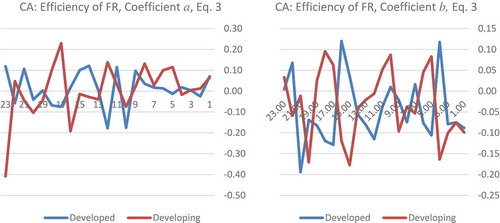
Graph 3 provides the trends of coefficients a and b. A careful look indicates that there is a slow trend toward 0 for coefficients a and b in both the panels and the values do not deviate much from 0, which again indicates that forecasters do try to learn from their past mistakes and incorporate new information in successive revisions.

Formal test results of forecast revision (Equation 3) are reported in Table 4. In this regression, we look at the correlation between two adjacent revisions, for example, between revisions 1 and 2, 2 and 3, 3 and 4, and so on. As we mentioned earlier, if the revisions were correlated, forecast errors would contain systematic information that could be used to improve the forecast. For efficiency, b should be zero, meaning forecasters should revise the current forecast based on the available information at present without being biased on the past revisions. They learn from the past mistakes and do not carry them over to the next period forecasts. An acceptance of the null hypothesis of b = 0 confirms that forecasters utilize all the information previously used efficiently to revise the forecast for the same target year. The null is accepted in only 4 and 6 cases for the developed and the developing country panels, respectively. In other words, forecast revisions are inefficient in general meaning forecasters could improve their forecasts by using information they used in the last period while revising the forecast for the next period. They carry over the last mistakes in their current revisions. Furthermore, we notice mostly negative correlations (b is negative) indicating that forecasters put less weight on the past revisions in their current forecast revisions. It also weakens the possibility of forecast smoothing as reported in some other studies. The results are stronger in the regression results of Equation 3 as the coefficient b is positive in only 2 cases for the developed country and in only 1 case for the developing country. We also report the results of the joint null hypothesis of a = 0, b = 0 and the results are mixed in both the panels indicating that forecast revisions not always random.

Table 4. Efficiency of forecast revision (Equation 3). $F{R}_{-i,t}=a+bF{R}_{-i-1,t}+e_{-i,t}$

		Developed				Developing
Horizon	Coef.	Value	Std. error	t-Prob.	F-Prob. a = 0. b = 0	Value	Std. error	t-Prob.	F-Prob. a = 0, b = 0
1 and 2	a	0.066	0.048	0.172		0.086	0.060	0.151
	b	−0.129	0.036	0.000	0.480	−0.364	0.072	0.000	0.001
2 and 3	a	−0.026	0.062	0.673		−0.005	0.051	0.922
	b	−0.573	0.054	0.000	0.000	−0.191	0.051	0.000	0.093
3 and 4	a	0.000	0.062	0.998		−0.002	0.063	0.976
	b	−0.246	0.118	0.038	0.602	−0.291	0.075	0.000	0.080
4 and 5	a	0.017	0.028	0.551		−0.024	0.052	0.643
	b	−0.087	0.035	0.013	0.993	−0.008	0.046	0.866	0.303
5 and 6	a	−0.018	0.044	0.690		0.183	0.068	0.008
	b	−0.101	0.039	0.010	0.308	−0.228	0.061	0.000	0.027
6 and 7	a	0.051	0.060	0.399		0.096	0.065	0.137
	b	−0.285	0.073	0.000	0.080	−0.316	0.070	0.000	0.056
7 and 8	a	−0.013	0.043	0.772		0.035	0.058	0.547
	b	−0.340	0.071	0.000	0.001	−0.130	0.034	0.000	0.013
8 and 9	a	0.019	0.034	0.562		0.134	0.109	0.223
	b	−0.015	0.040	0.710	0.132	−0.166	0.085	0.053	0.223
9 and 10	a	0.095	0.045	0.035		−0.032	0.083	0.698
	b	−0.073	0.032	0.023	0.000	−0.023	0.038	0.553	0.779
10 and 11	a	−0.106	0.060	0.077		0.031	0.123	0.800
	b	−0.567	0.039	0.000	0.000	−0.426	0.048	0.000	0.000
11 and 12	a	0.102	0.083	0.221		−0.105	0.167	0.532
	b	0.090	0.066	0.169	0.533	0.074	0.091	0.414	0.841
12 and 13	a	−0.158	0.070	0.025		0.145	0.115	0.210
	b	−0.375	0.075	0.000	0.003	−0.583	0.095	0.000	0.000
13 and 14	a	0.078	0.049	0.114		0.003	0.079	0.967
	b	−0.293	0.040	0.000	0.000	−0.208	0.055	0.000	0.522
14 and 15	a	0.118	0.068	0.084		−0.044	0.093	0.641
	b	−0.171	0.046	0.000	0.200	−0.314	0.078	0.000	0.129
15 and 16	a	0.111	0.080	0.168		−0.017	0.080	0.835
	b	−0.549	0.115	0.000	0.006	−0.149	0.060	0.014	0.266
16 and 17	a	−0.018	0.039	0.652		−0.122	0.090	0.175
	b	−0.188	0.051	0.000	0.526	−0.105	0.061	0.087	0.330
17 and 18	a	−0.059	0.043	0.170		0.275	0.089	0.002
	b	0.022	0.028	0.442	0.562	−0.442	0.065	0.000	0.001
18 and 19	a	−0.045	0.086	0.597		0.067	0.088	0.449
	b	−0.286	0.099	0.004	0.207	−0.352	0.082	0.000	0.192
19 and 20	a	−0.019	0.045	0.670		−0.083	0.073	0.257
	b	−0.132	0.046	0.004	0.000	−0.057	0.069	0.414	0.719
20 and 21	a	−0.023	0.052	0.664		−0.086	0.070	0.226
	b	−0.302	0.043	0.000	0.000	−0.084	0.053	0.114	0.816
21 and 22	a	0.112	0.068	0.100		−0.087	0.090	0.331
	b	−0.063	0.045	0.163	0.237	−0.007	0.046	0.875	0.798
22 and 23	a	−0.037	0.075	0.617		−0.155	0.103	0.134
	b	−0.378	0.040	0.000	0.000	−0.505	0.040	0.000	0.000

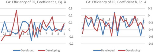
Graph 4 depicts the trends in these two coefficients. We notice a slow trend toward 0 in coefficient a, but no such trend in b. Coefficient b remains below 0 in both the panels in almost all the horizons.

6. Conclusions and discussions

In this paper, we test accuracy, unbiasedness and efficiency of expert expectations of CA share in GDP for two panels of 25 developed and 18 developing countries following the methodologies in the existing literature. We use a consensus based survey data set previously unexploited by researchers. We compare the results between the two panels and discuss them in the paper.

Forecast accuracy measures reveal that the magnitude of the forecast error declines as the forecast horizons get closer to the actual realization in both the panels. Forecast absolute errors and root mean squared errors are larger for the developing country panel. TICs suggest that consensus forecast performs better than a naive forecast.

Results of Equation 1 indicates mixed results between the two panels. Forecast errors are unbiased (a = 0) but inefficient (b = 0) across almost all the horizons for the developed country. Schuh (2001) also found similar results using US data. On the other hand, forecast errors are strongly biased but weakly efficient (as half of the b = 0 hypothesis cannot be rejected) for the developing country. However, the joint null of a = 0, b = 0 is strongly rejected for both the panels. By looking at the significance of b = 0, we may say that forecasters are better able to use information in their forecasts for the developing country than the developed country as the null of b = 0 is accepted in almost half the regressions in the developing country panel compared to only two in the developed country panel. In other words, forecasts of the developing country are more efficient. By looking at the trends of the two coefficients, we conclude that forecasters do actively try to minimize errors as both the a and the b coefficients consistently move toward 0 over time. However, the developing country coefficients are more disperse than the developed country.

We perform two tests of efficiency of forecast revisions. In the first test, we investigate if forecasters were able to incorporate information they used in an earlier forecast (a year early) for the same horizon. Formal test results indicate acceptance of efficiency as the null of b = 0 is accepted across most horizons in both the panels. In other words, there is no horizon specific bias in the forecast. It could also mean that forecasters did not forget the mistakes they made previously to forecast the same horizon. They used the past information efficiently. It may also mean that a year-old information is too old in CA forecasting. Forecasters are more concerned about more recent information. In the second regression of forecast revisions, we look into the correlation between the two adjacent revisions. Efficiency is rejected in general for both the panels. In other words, forecasters could improve their forecasts by using information they used in the last period while revising the forecast for the next period. Although these two results seem contradictory, they should not be taken as a contradiction. Forecasters may be successful in incorporating information in one dimension, but may not be successful to do so in another dimension. Monthly forecast revisions are expected to be correlated as it does not provide enough time to understand the mistakes made a month early. However, as the time passes by, for example, a mistake made a year early is easier to detect and rectify. Additionally, we notice fewer positive correlations (positive b) in both the regressions across various horizons, which suggest less forecast smoothing contrary to the findings in some earlier studies. In fact, we observe many significant negative b values. A significant negative coefficient estimate indicates that forecasters were not conservative in revising their forecasts, and it might also mean that forecasters put less weight on the past revisions. A careful look at the graphs of the coefficients from both the regressions indicates that there is a slow trend toward zero for the coefficient a. But the trend in b is not always clear. Overall we can say that forecasters do improve their forecasts as the horizons become shorter, but the forecasts fall short of being efficient and in some cases unbiased statistically.

Our results show some differences in the results between the two panels which we believe should not be surprising. These types of differences do exist in other areas as well, for example, financial market efficiency in developed and developing countries. Forecasting of developing countries might be relatively easier for some variables, but may also be difficult for some other variables depending on the availability and the quality of data. Developed country markets and institutions are highly developed and thus, data are of high-quality, reliable, timely and accessible. However, forecasting may be more complicated as many economic relations are complicated relative to the developing country. Genberg and Martinez (2014) provides a perspective from their study in which they conclude, “forecast performance for low-income countries may reflect less the ability of the forecaster than the lack of information. From the point of view of being able to foresee economic troubles and propose appropriate policy responses, there seems to be a high payoff to improving data availability in these cases. It is possible that the relatively poor record in forecasting recessions in low-income countries could be the consequence of a lack of attention and resources allocated to developing forecast and early-warning methodologies specific to these types of economies”. High-quality forecast requires high-quality data and forecaster. Policy makers should strive to build a forecasting infrastructure keeping in mind these shortcomings.

Graph 1. Descriptive statistics of CA forecast error.

Graph 2. Efficiency of forecast error, trends in coefficients a and b (Equation 1).

Graph 3. Efficiency of forecast revisions: trends in coefficients a and b (Equation 2).

Graph 4. Efficiency of forecast revisions: trends in coefficients a and b (Equation 3).

Acknowledgments

The first author would like to thank participants at the Department of Finance and Economics Conference Day presentation, November 2016, for valuable discussions on the paper. Both authors would like to thank participants at the Eastern Economic Association (EEA) Meeting 2017, NYC for valuable comments and suggestions on an earlier draft of the paper.

Additional information

Funding

This work was supported by Deanship of Scientific Research (DSR) of the King Fahd University of Petroleum and Minerals (KFUPM) [grant number IN141045 to FM].

Notes on contributors

Fazlul Miah

Fazlul's research interests are primarily in the area of financial markets and international finance although he has contributed to other areas as well. The current article comes out of a larger project on understanding forecasting performance of professional forecasts of key macroeconomic variables. One particular focus of the project is to understand if there are significant differences between the developed and developing country forecasts. The issue is an important one because of the extensive use of forecast data to make plans for the future by various government agencies and business entities.

Notes

1. These are opinions of experts. Consensus or average forecasts are considered better than individual forecast. The history of expert-survey opinion collection goes back to 1946, when Joseph Livingston, a journalist, first started to ask a number of economists their expectations of inflation over the coming year and the coming five years. Now, the Federal Reserve Bank of Philadelphia conducts this survey. See Pesaran and Weale (2006) for further details on the general history of survey data.

2. Because of its importance, a number of newspapers, including the Wall Street Journal, the Economist, Financial Times, etc. collect and publish expert opinions on important macroeconomic and financial variables.

3. We explain the meanings of unbiasedness and efficiency in the methodology section.

4. Current account as a percentage of GDP to be more precise.

5. In a fixed event forecast, a series of forecasts are made at certain intervals (for example, every month, every quarter, etc.) about a target variable until the actual realization of the event happens at a fixed time in the future. Further discussions about fixed event forecast and its econometrics properties are available in Nordhaus (1987).

6. Further discussions of advantages and disadvantages of each of these measures are available in Bowles et al. (2007).

7. Holden, Peel, and Sandhu (1987) demonstrate that a test of a = 0 provides a sufficient, but not a necessary condition for unbiasedness.

8. Berger and Krane (1985) provide econometric discussions of these two equations.

9. These interpretations are taken from Ashiya (2006).

10. Loungani (2001) uses the same technique. We avoided discussions of these techniques in the paper to save space. These discussions are available in many Econometric textbooks. We tried various combinations of fixed and random effects in the regressions. However, we do not notice significant changes in the results.

11. http://www.un.org/en/development/desa/policy/wesp/wesp_current/2014wesp_country_classification.pdf. Page 3.

12. We also compute the results of the full panel. Results of the full panel are available upon request.

13. We perform the unbiasedness test as suggested by Holden et al. (1987) and the results are reported in Table A1. In general, there are no differences in the results between these two methods. We also performed a direct test of unbiasedness following Loungani (2001) and Swidler and Ketcher (1990), and the results indicate that forecasts are biased in general. We produce these results in Table A2. We do not focus on these two methods as these methods seem less utilized in the literature.

Appendix

Table A1. Test of bias in forecast. $F{E}_{i,t}=C+e_{i,t}$

		Developed			Developing
Horizon	Constant	Value	Std. error	t-Prob.	Value	Std. error	t-Prob.
1	C	0.041	0.089	0.646	−0.496	0.156	0.002
2	C	−0.035	0.087	0.686	−0.580	0.146	0.000
3	C	−0.049	0.091	0.590	−0.584	0.154	0.000
4	C	−0.007	0.098	0.942	−0.579	0.156	0.000
5	C	−0.026	0.102	0.799	−0.556	0.163	0.001
6	C	−0.002	0.103	0.981	−0.713	0.170	0.000
7	C	−0.058	0.108	0.589	−0.804	0.177	0.000
8	C	−0.040	0.104	0.703	−0.821	0.172	0.000
9	C	−0.058	0.102	0.573	−0.960	0.195	0.000
10	C	−0.164	0.107	0.127	−0.926	0.201	0.000
11	C	−0.009	0.122	0.944	−0.999	0.246	0.000
12	C	−0.098	0.117	0.404	−0.815	0.230	0.001
13	C	0.078	0.121	0.518	−0.953	0.198	0.000
14	C	0.029	0.125	0.814	−0.966	0.208	0.000
15	C	−0.069	0.119	0.562	−0.921	0.229	0.000
16	C	−0.183	0.144	0.205	−0.926	0.236	0.000
17	C	−0.177	0.147	0.230	−0.779	0.223	0.001
18	C	−0.117	0.143	0.417	−1.012	0.218	0.000
19	C	−0.075	0.127	0.555	−1.107	0.228	0.000
20	C	−0.062	0.127	0.627	−1.029	0.227	0.000
21	C	−0.004	0.133	0.976	−0.950	0.231	0.000
22	C	−0.121	0.136	0.377	−0.862	0.218	0.000
23	C	−0.048	0.152	0.751	−0.977	0.255	0.000

Each cell reports the results of a regression of forecast errors on a constant.

Table A2. Unbiasedness of forecast. $A_t=a+b{F}_{-i,t}+e_{-i,t}$

		Developed				Developing
Horizon	Coefficient	Value	Std. error	t-Prob.	F-Prob. a = 0, b = 1	Value	Std. error	t-Prob.	F-Prob. a = 0, b = 1
1	a	0.066	0.088	0.452	0.000	1.005	0.230	0.000
	b	0.798	0.036	0.000		0.813	0.063	0.000	0.000
2	a	0.128	0.087	0.141	0.000	0.964	0.208	0.000
	b	0.834	0.035	0.000		0.850	0.059	0.000	0.000
3	a	0.151	0.090	0.095	0.000	1.058	0.224	0.000
	b	0.818	0.037	0.000		0.811	0.064	0.000	0.000
4	a	0.131	0.098	0.184	0.000	1.063	0.226	0.000
	b	0.790	0.041	0.000		0.811	0.064	0.000	0.000
5	a	0.150	0.101	0.141	0.000	1.195	0.231	0.000
	b	0.782	0.043	0.000		0.752	0.065	0.000	0.000
6	a	0.138	0.102	0.178	0.000	1.313	0.248	0.000
	b	0.772	0.043	0.000		0.752	0.076	0.000	0.000
7	a	0.200	0.106	0.061	0.000	1.572	0.241	0.000
	b	0.740	0.046	0.000		0.671	0.073	0.000	0.000
8	a	0.165	0.104	0.112	0.000	1.459	0.238	0.000
	b	0.774	0.045	0.000		0.724	0.073	0.000	0.000
9	a	0.169	0.102	0.098	0.000	2.003	0.233	0.000
	b	0.792	0.045	0.000		0.521	0.069	0.000	0.000
10	a	0.272	0.105	0.010	0.000	2.070	0.234	0.000
	b	0.750	0.046	0.000		0.483	0.068	0.000	0.000
11	a	0.237	0.113	0.037	0.000	2.663	0.238	0.000
	b	0.611	0.044	0.000		0.221	0.065	0.001	0.000
12	a	0.234	0.110	0.034	0.000	2.348	0.248	0.000
	b	0.722	0.048	0.000		0.353	0.071	0.000	0.000
13	a	0.149	0.119	0.212		1.839	0.251	0.000
	b	0.677	0.050	0.000	0.000	0.575	0.081	0.000	0.000
14	a	0.206	0.120	0.088		2.008	0.252	0.000
	b	0.641	0.050	0.000	0.000	0.497	0.079	0.000	0.000
15	a	0.226	0.118	0.056		2.318	0.258	0.000
	b	0.719	0.053	0.000	0.000	0.341	0.078	0.000	0.000
16	a	0.409	0.128	0.002		2.430	0.261	0.000
	b	0.490	0.051	0.000	0.000	0.288	0.078	0.000	0.000
17	a	0.415	0.130	0.002		2.239	0.284	0.000
	b	0.470	0.052	0.000	0.000	0.354	0.089	0.000	0.000
18	a	0.373	0.130	0.004		2.258	0.276	0.000
	b	0.497	0.053	0.000	0.000	0.385	0.094	0.000	0.000
19	a	0.269	0.124	0.031		2.464	0.270	0.000
	b	0.647	0.057	0.000	0.000	0.298	0.092	0.001	0.000
20	a	0.255	0.125	0.042		2.444	0.278	0.000
	b	0.658	0.058	0.000	0.000	0.296	0.095	0.002	0.000
21	a	0.259	0.127	0.042		2.513	0.283	0.000
	b	0.590	0.055	0.000	0.000	0.252	0.094	0.008	0.000
22	a	0.344	0.127	0.007		2.183	0.283	0.000
	b	0.558	0.055	0.000	0.000	0.393	0.092	0.000	0.000
23	a	0.374	0.132	0.005		2.776	0.265	0.000
	b	0.435	0.051	0.000	0.000	0.128	0.081	0.114	0.000

References

- Abarbanell, J. S., & Bernard, V. L. (1992). Tests of analysts’ overreaction/underreaction to earnings information as an explanation for anomalous stock price behavior. Journal of Finance, 47, 1181–1207. doi:10.1111/j.1540-6261.1992.tb04010.x
- Ager, P., Kappler, M., & Osterloh, S. (2009). The accuracy and efficiency of the consensus forecasts: A further application and extension of the pooled approach. International Journal of Forecasting, 25, 167–181. doi:10.1016/j.ijforecast.2008.11.008
- Amir, E., & Ganzach, Y. (1998). Overreaction and underreaction in analysts’ forecasts. Journal of Economic Behavior and Organization, 37, 333–347. doi:10.1016/S0167-2681(98)00092-4
- Ashiya, M. (2002). Accuracy and rationality of Japanese institutional forecasters. Japan and the World Economy, 14, 203–213. doi:10.1016/S0922-1425(02)00004-X
- Ashiya, M. (2003). Testing the rationality of Japanese GDP forecasts: The sign of forecast revision matters. Journal of Economic Behavior and Organization, 50, 263–269. doi:10.1016/S0167-2681(02)00051-3
- Ashiya, M. (2006). Testing the rationality of forecast revisions made by the IMF and the OECD. Journal of Forecasting, 25, 25–36. doi:10.1002/(ISSN)1099-131X
- Bakshi, H., & Yates, A. 1998. Are UK inflation expectations rational? Bank of England Working Paper No. 81.
- Batchelor, R. (2007). Bias in macroeconomic forecasts. International Journal of Forecasting, 23, 189–203. doi:10.1016/j.ijforecast.2007.01.004
- Berger, A. N., & Krane, S. D. (1985). The informational efficiency of econometric model forecasts. Review of Economics and Statistics, 67, 667–674.
- Boero, G., Smith, J., & Wallis, K. F. (2008). Evaluating a three-dimensional panel of point forecasts: The Bank of England Survey of External Forecasters. International Journal of Forecasting, 24, 354–367. doi:10.1016/j.ijforecast.2008.04.003
- Bowles, C., Friz, R., Genre, V., Kenny, G., Meyler, A., & Rautanen, T. 2007. The ECB survey of professional forecasters (SPF): Review after eight years’ experience. Occasional paper series 59. European Central Bank.
- Chen, Q., Costantini, M., & Deschamps, B. (2016). How accurate are professional forecasts in asis? Evidence from ten countries. International Journal of Forecasting, 32, 154–167. doi:10.1016/j.ijforecast.2015.05.004
- Clements, M. P. (1995). Rationality and the role of judgment in macroeconomic forecasting. Economic Journal, 105, 410–420. doi:10.2307/2235500
- Clements, M. P. (1997). Evaluating the rationality of fixed-event forecasts. Journal of Forecasting, 16, 225–239. doi:10.1002/(ISSN)1099-131X
- Dovern, J., & Weisser, J. (2011). Accuracy, unbiasedness and efficiency of professional macroeconomic forecasts: An empirical comparison for the G7. International Journal of Forecasting, 27, 452–465. doi:10.1016/j.ijforecast.2010.05.016
- Ehrbeck, T., & Waldmann, R. (1996). Why are professional forecasters biased? Agency versus behavioral explanations. Quarterly Journal of Economics, 111, 21–40. doi:10.2307/2946656
- Gallo, G. M., Granger, C. W., & Jeon, Y. (2002). Copycats and common swings: The impact of the use of forecasts in information sets. IMF Staff Papers, 49, 4–21.
- Genberg, H. & Mertinez, A. (2014). On the accuracy and efficiency of IMF forecasts: A survey and some extensions. Retrieved from http://www.ieo-imf.org/ieo/files/completedevaluations/BP-14-04.pdf
- Harvey, D. I., Leybourne, S. J., & Newbold, P. (2001). Analysis of a panel of UK macroeconomic forecasts. Econometrics Journal, 4, S37–S55. doi:10.1111/1368-423X.00052
- Holden, K., Peel, D., & Sandhu, B. (1987). The accuracy of OECD forecasts. Empirical Economics, 12, 175–186. doi:10.1007/BF01973428
- Isiklar, G., Lahiri, K., & Loungani, P. (2006). How quickly do forecasters incorporate news? Evidence from cross-country surveys. Journal of Applied Econometrics, 21(6), 703–725. doi:10.1002/(ISSN)1099-1255
- Jongen, R., & Verschoor, W. F. C. (2007). Further evidence on the rationality of interest rate expectations. Journal of International Financial Markets, Institutions, and Money, 18, 438–448. doi:10.1016/j.intfin.2007.05.003
- Jongen, R., Verschoor, W. F. C., & Wolff, C. C. P. (2008). Foreign exchange rate expectations: Survey and synthesis. Journal of Economic Surveys, 22, 140–165. doi:10.1111/j.1467-6419.2007.00523.x
- Loungani, P. (2001). How accurate are private sector forecasts? Cross-country evidence from consensus forecasts of output growth. International Journal of Forecasting, 17, 419–432. doi:10.1016/S0169-2070(01)00098-X
- Loungani, P., Stekler, H., & Tamirisa, N. (2013). Information rigidity in growth forecasts: Some cross-country evidence. International Journal of Forecasting, 29, 605–621. doi:10.1016/j.ijforecast.2013.02.006
- Miah, F., Khalifa, A., & Hammoudeh, S. (2016). Further evidence on the rationality of interest rate expectations: A comprehensive study of developed and emerging economies. Economic Modelling, 54, 574–590. doi:10.1016/j.econmod.2015.12.036
- Nordhaus, W. D. (1987). Forecasting efficiency: Concepts and applications. Review of Economics and Statistics, 69, 667–674. doi:10.2307/1935962
- Pesaran, M. H., & Weale, M. (2006). “Survey expectations.” In G. Elliott, C. W. Granger, & A. Timmermann (Eds..), Handbook of economic forecasting (Vol. 1, pp. 715-776). North-Holland, Amsterdam: Elsevier (North Holland Publishing Company).
- Schuh, S. (2001). An evaluation of recent macroeconomic forecast errors. New England Economic Review, (1), 35-56. January/February 2001.
- Stekler, H. O. (2002). The rationality and efficiency of individuals’ forecasts. In M. P. Clements & D. F. Hendry (Eds.), A companion to economic forecasting (pp. 222-240). Oxford: Blackwell Publishers Inc.
- Swidler, S., & Ketcher, D. (1990). Economic forecasts, rationality, and the processing of new information over time. Journal of Money, Credit and Banking, 22, 65–76. doi:10.2307/1992128
- Timmermann, A. (2007). An evaluation of the World Economic Outlook Forecasts. IMF Staff Papers, 54, 1–33. doi:10.1057/palgrave.imfsp.9450007
Appendix
Table A1. Test of bias in forecast.
Table A2. Unbiasedness of forecast.