Do sentiment indices impact the premium of prominent pricing factors?

Abstract

This study investigates whether Google Search Volume Indices (GSVIs) bring shifts in the expected return of prominent pricing factors in comparison to the Volatility Index (VIX). The results show that compared to VIX, GSVIs bring less significant changes in expected premium on Fama–French’s five-factors and q-factors. Pessimistic sentiment indices (Market Crash and Bear Market) predict more significant variation in the premium of prominent pricing factors than optimistic sentiment indices (Market Rally and Bull Market), and also have a significant correlation with VIX representing downside risk. Furthermore, the sentiment indices are better in predicting premium on five-factors than q-factors.

Keywords:

• VIX
• Google search index
• expected return
• asset pricing
• pricing factors

JEL classification:

• G12
• C19

PUBLIC INTEREST STATEMENT

Predicting investor behavior is crucial in determining prices of securities, and premiums on pricing factors. Advent of internet has brought new set of investor sentiments data in the shape of internet searches of terms defining investor behavior. We use Volatility Index (VIX) and Google Search Volume Index (GSVI) as proxy for investors’ sentiments to analyze the impact of sentiments on premium of pricing factors included in Fama and French (2015) five factor model and Hou et al. (2015) q-factor model. In our findings, sentiments impact on the pricing of securities by bringing variations in pricing factor premiums, in fact, VIX is found more robust than GSVIs. Thus investors’ should consider sentiments along with firm specific and fundamental variables in pricing securities. Furthermore, in ascertaining the external shocks impact, the Fama and French five factors are found more robust in explaining the variance of q-factors but not vice versa.

1. Introduction

The equilibrium asset pricing models such as Intertemporal Capital Asset Pricing Model (ICAPM) (Merton, 1973), and Arbitrage Pricing Model (APM) (Ross, 1976) imply that expected excess returns should vary with exposure to multiple factors instead of the single market factor of Capital Asset Pricing Model (CAPM) (Sharpe, 1964; Lintner, 1965; Mossin, 1966). Recently, Fama and French (2015) proposed a five-factor model and Hou, Xue, and Zhang (2015) proposed a q-factor model. It was found that these models performed better than Fama and French (1993) three-factor model and Carhart (1997) four-factor model. These models assume that investors are rational, and market information is quickly adjustable to stock prices. However, previous literature also provides the evidence of another class of investors, known as irrational traders, which are prone to exogenous sentiments (Baker and Wurgler, 2007). However, the impact of investor sentiments on the asset pricing models is relatively less explored in the extant literature. We address this issue in the paper by empirically testing whether factor returns can be predicted using Google search volume indices (GSVIs).

Research on behavioural finance advocates that the investors’ behaviour plays an important role in determining stock prices. Fisher and Statman (2000) find a negative relationship between investor sentiment and future stock returns, suggesting that sentiments can influence the stock market returns. Similarly, sentiments also impact securities that are difficult to arbitrage and sentiments enhance the performance of the factors that predict stock returns (Baker & Wurgler, 2006). Bandopadhyaya and Jones (2006) stated that sometimes the investor behaviour (investor sentiments) predict prices better than other fundamental factors. The sentiment index referred as “investor fear gauge”, the market volatility index (VIX) is also found to be related to stock market returns (Fleming, Ostdiek, & Whaley, 1995; Giot, 2005, Whaley, 2000, 2009). Durand, Lim, and Zumwalt (2011) investigate whether shift in VIX bring any change in expected returns on Fama and French (1993) three factors [market portfolio excess return (Rm-Rf), high minus low book-to-market portfolio (HML), and small minus big size portfolio (SMB)] along with the momentum factor [winners minus losers (WML)] proposed by Carhart (1997). Authors find that changes in VIX have the larger effect on Rm-Rf and HML than SMB and WML. We go step further to examine the effect of GSVIs and VIX to determine variations in the expected return of the pricing factors included in Fama–French five-factor and q-factor model.

This study employs shifts in four GSVIs [market crash (D_Crash), bear market (D_Bear), bull market (D_Bull), and market rally (D_Rally)] because they capture the extreme events and the market variations. Klemola, Nikkinen, and Peltomäki (2016) employ GSVIs to examine the relationship between investors’ market attention and stock market returns. They find that these measures of market attention are potential gauges for investor sentiment. Habibah, Rajput, and Sadhwani (2017) used the pessimistic investor sentiments (market crash and bear market) to predict the stock returns. VIX is also used as a measure of sentiment because it has been considered as a leading indicator of investor sentiment and realized market volatility in the literature. Market sentiment is the attitude of investors toward a particular security or financial market. Change in attitude of investors may bring change in stock prices and ultimately affecting the wealth of investors. The sentiment index has more effect on securities whose value is difficult to arbitrage and whose valuation is highly subjective (Baker & Wurgler, 2006).

To investigate changes in the premium of pricing factors included in the five-factor model and q-factor model, we use standard methodologies such as Granger Causality (1969), Vector Auto-regression, Variance Decomposition and Impulse Response Function. The findings show that changes in VIX (D_VIX) Granger cause variation in all factors included in the q-factor model and in the five-factor model except HML. Also, the changes in GSVIs (except market rally) Granger cause variation in all factors, however, the significance of VIX is higher than GSVIs.

Further, this study tests whether GSVIs show Monday effect or not (see, appendix for results). We follow Ülkü (2017), who found that Fama and French’s RMW factor premium is because of Monday effect. To test this effect, we create a dummy to test the day effect where numbers are assigned for the days from 1 to 5 (Monday = 1, Tuesday = 2, Wednesday = 3, Thursday = 4, Friday = 5). Table A1 shows the results of Monday effect on the RMW along with GSVIs. The results of Table A1 (a–d) depict that the premium on RMW factor is a Monday effect but it is not subsumed by GSVIs as it remains significant after controlling for GSVIs.

The remainder of the study is organized as follows. The next section presents the literature review and hypothesis development. Section 3 describes the data, methodology and descriptive statistics. Empirical results and discussion is provided in Section 4, while Section 5 concludes the paper.

2. Literature review

Investor sentiment is broadly studied in the literature to address the major issue that whether investor sentiment does have an effect on stock returns and can it forecast the expected return on stocks. For that researchers have used variety of sentiment measures such as Simon and Wiggins III (2001) and Wang, Keswani, and Taylor (2006) have used put-call ratio, Lee, Shleifer, and Thaler (1991), Chen, Kan, and Miller (1993), Swaminathan (1996), Neal and Wheatley (1998), Elton, Gruber, and Busse (1998), and Brown and Cliff (2005) have used closed-end fund discounts, Neal and Wheatley (1998), Brown et al. (2003), Brown and Cliff (2005), Frazzini and Lamont (2008) and Ben-Rephael, Kandel, and Wohl (2012) have used mutual fund data. Among others, Randall, Suk, and Tully (2003) have used Net Cash Flow into Mutual Funds, Lashgari (2000) have used the Barron’s Confidence Index, Baker and Wurgler (2006) employs the issuance Percentage, Whaley (2000) has employed the VIX-Investor Fear Gauge, and Kumar and Persaud (2002) have employed the Risk Appetite Index (RAI).

Klemola et al. (2016) have used Google Search Volume Index for Google search terms “market crash, bear market, bull market, and market rally” to predict near-term future stock returns. Habibah et al. (2017) have used the pessimistic GSVIs and VIX to predict the stock returns. To forecast patterns of market activity, pessimistic media content variables are used by Tetlock (2007), whereas Preis, Moat, and Stanley (2013) have used Google search terms to predict movements in the equity market.

VIX is used to measure investors’ expectation of market volatility and its effect on stock returns. Whaley (2000) finds the negative relationship between stock market returns and VIX. Simon and Wiggins III (2001) recognize that variations in VIX may forecast the market and stock returns. Fleming et al. (1995), Whaley (2000), (2009) and Giot (2005) find negative the relationship between stock returns and changes in VIX. They find that increases in volatility cause decrease in return on S&P500 index. There is a significant empirical evidence that VIX is used as a good predictor for future market volatility (Whaley, 2000; Blair, Poon, & Taylor, 2001; Engle & Gallo, 2006; Dennis & Strickland, 2002; Giot & Laurent, 2007; Habibah et al., 2017). Sarwar (2012) examines the relationship between VIX and Stantdard and Poor’s (S&P) 100, 500 and 600 indices returns and finds the negative relationship between VIX and return on indices. Durand et al. (2011) examine that whether the variations in Fama and French three-factor model augmented with a momentum factor are driven by changes in VIX and find that market risk premium and the value premium are more sensitive to the changes in VIX.

We use GSVIs for four search terms: market crash, bear market, bull market, and market rally (first two terms show pessimistic (negative) sentiments, whereas the latter two terms show optimistic (positive) sentiments of investors). We also use VIX to estimate variations in the expected returns for Fama–French five-factor model and q-factor model.

2.1. Fama–French five factor model

Motivated by valuation theory, Fama and French (2015) proposed the five-factor model by including two new variables in Fama–French three-factor model to explain variations in the expected return on a stock portfolio. The five-factor model given in equation (1) below includes market risk premium (Rm-Rf), size factor (SMB), value factor (HML), investment (CMA), and profitability (RMW).

(1) $R_{it}-R_{ft}={\alpha }_i+{\beta }_1\left(RM-R_{ft}\right)+{\beta }_2\left(SM{B}_t\right)+{\beta }_3\left(HM{L}_t\right)+{\beta }_4\left(RM{W}_t\right)+{\beta }_5\left(CM{A}_t\right)+{ϵ}_{it}$(1)

The market risk premium (Rm-Rf) is excess of return over risk-free rate. The risk-free rate is the minimum return that the investors want to receive on investment and Treasury-bill rate proxies for the risk-free rate. When an investor invests in any stock then he/she wants to receive more return than the risk-free rate, which is called the market risk premium.

SMB, a size factor, is the return on small stocks minus big stock’s portfolio. Banz (1981) found that size characteristics explain the variation in returns, and determines that there is a negative relationship between size and expected return. Market capitalization (price per share times number of shares outstanding) is used as a proxy to measure the size of a firm. HML, value factor is the return on value stocks [high book to market equity (ME)] minus return on growth stock’s (low book to market equity) portfolio. Rosenberg, Reid, and Lanstein (1985) demonstrated the direct relationship between expected stock returns and book to market equity. Whereas Chan, Hamao, and Lakonishok (1991) find that the variation in the expected return on Japanese stocks is explained by book to market equity.

CMA, investment factor, is the stock return of companies that invest conservatively minus stock return of companies that invest aggressively. Aharoni, Grundy, and Zeng (2013), and Fama and French (2006) examined the negative relationship between average return and investment. Asset growth is used as a proxy to measure investment of firm. RMW, a profitability factor, is the return on stocks with robust profitability and return on stocks with weak profitability. Novy-Marx (2013) found that despite having high valuation ratios, return on the profitable firm is higher than unprofitable firms. Here, operating profitability (revenue minus operating expenses) is used as a proxy to measure the profitability of a firm.

2.2. Q-factor model

Motivated by the neo-classical q-theory of investment, Hou et al. (2015) proposed the q-factor model that explains the variations in average stock returns. The q-factor model specification is as follows:

(2) $R_{it}-R_{ft}={\alpha }_i+{\beta }_1\left(RM-R_{ft}\right)+{\beta }_2\left(M{E}_t\right)+{\beta }_3\left(IA\right)+{\beta }_4\left(RO{E}_t\right)+{\epsilon }_{it}$(2)

Where market risk premium is the excess return over risk-free rate (Rm-Rf); here Treasury bill rate is taken as a proxy for the risk-free rate. The Size factor is the difference between the return on stocks having small Market Equity (ME) and return on stocks having big ME. ME is measured as stock price times the number of shares outstanding. Investment factor is the difference between the return on stocks having the low investment and the return on stocks having the high investment (IA), in which investment to asset ratio (annual change in total assets) is used as a proxy to measure investment of firm. Profitability is the difference between the return on stocks having the high return on equity (ROE) and the return on stocks having the low ROE. ROE (income before extraordinary items) is used as a proxy to measure the profitability of a firm.

Though the factors are the same except HML in both models but they are different in the construction and proxies, mainly for investment and profitability. The Fama–French five-factors are constructed from two (2x3) sort by interacting size with operating profitability and investment. Whereas, q-factors are constructed from three (2x3x3) sort on size, investment, and profitability. Hou, Xue, and Zhang (2014) compare q-factor model and Fama–French five-factor model and discuss few major concern regarding the composition of factors (see. Hou et al., 2014). They find that empirically q-factor model outperform Fama–French five-factor model. We are using both recently proposed models in our study to examine the effect of investor’s sentiment on risk premium of pricing factors included in models. It will be helpful for investors to know which model is capturing the effect of investors’ sentiment.

2.3. Hypotheses development

Findings of Durand et al. (2011) show that the variation in the expected return of Fama–French three factors along with momentum are predicted by changes in VIX. The study period of Durand et al. (2011) ends in 2007 and since then there is an increase in the number of pricing factors in the prominent equity pricing models. Recently, two competing models have been introduced, the first model is the extension of the Fama–French three-factor model by augmenting it with the investment and profitability factor. This model is called Fama and French (2015) five-factor model. The other competing model includes four-factors, and this model is motivated by the q-theory of investment. This model is introduced by the Hou et al. (2015), and they claim that it is a better model than the Fama and French (2015) five-factor model. Thus, in the spirit of the Durand et al. (2011), there is a need to test whether the expected return on factors of these two model is impacted by any changes in the VIX. Our first hypothesis is:

H1: Change in VIX impacts the risk premium on pricing factors included in Fama–French (2015) five-factor and Hou et al. (2015) q-factor model.

Other sentiment indices which are used to predict variation in expected return are GSVIs. Four search terms: Bear market, Market crash, Market rally and Bull market are used to measuring investor sentiments. First two terms measure negative sentiments while the other two measure positive sentiments. These search terms were used by Klemola et al. (2016) to measure changes in investors’ market attention. Because of economic uncertainty, investors are more concerned about the risk and return on their investment, and they try to minimize the risk by selling (buying) stocks if stock prices are expected to go down (up). Market crash and bear market are the terms that investors use when there is an economic downturn and stocks’ prices fall, whereas bull market and market rally are the terms that investors use when there is an economic boom and stock prices go up. It is also well-known that uncertainty about the future has implications on economic agents’ behaviour (Bloom, 2009; Bloom, Bond, & Van Reenen, 2007; Dixit, 1989). Literature provides evidence that economic uncertainty affects financial markets, especially firm fundamentals, such as cash flows, risk-adjusted discount factors, investment opportunities (Bloom, 2009; Bloom et al., 2007), and equity portfolios and individual stocks (Anderson, Ghysels, & Juergens, 2009; Bali & Zhou, 2016; Bekaert, Hodrick, & Zhang, 2009).

Small firms are relatively more sensitive to economic downturns than large firms (e.g., Fort, Haltiwanger, Jarmin, & Miranda, 2013; Gertler & Gilchrist, 1994), investors incline to move towards large stocks when the market goes down. Therefore, the expected relationship between SMB and market crash/bear market indices is negative. Value stocks are riskier than growth stocks in the time of economic downturn (e.g., Lettau & Ludvigson, 2001; Petkova & Zhang, 2005; Zhang, 2005), suggesting that investors try to move from value stocks to growth stocks to have safer investment. Therefore the expected relationship between HML and market crash/bear market indices is negative.

Titman, Wei, and Xie (2004) advocated that abnormal capital investment has a negative relationship with the expected stock return and this relation is strong for those firms that have high cash flows. The expected relationship between CMA and market crash/bear market is positive indicating robust returns for firms with conservative investment than firms with aggressive investments Novy-Marx (2013) demonstrated that profitable firms are less prone to distress. Therefore the expected relationship between RMW and market crash/bear market is positive. The relationship of these factors is expected to be positive for the bull market and market rally indices that depict positive investor sentiments except CMA. Therefore, hypothesis two is constructed to examine the impact of GSVIs on Fama–French five-factors and q-factors.

H2: Change in GSVIs (market crash, market rally, bear market and bull market) impacts the premium of pricing factors included in Fama–French five-factor and q-factor models.

3. Data and methodology

This study employs GSVIs data for four search terms which represent investor sentiments. The search terms include Bear Market, Bull Market, Market Rally and Market Crash. GSVIs daily data is used for the period from January 2004 to December 2014, downloaded from https://www.google.com/trends/. GSVI measure shows how many searches have been done for a specific search term on Google web search on a specific day relative to the total number of searches done for the same specific search term on Google web search over time.

We obtain the VIX daily data from http://www.cboe.com. VIX measures the expected market volatility of the S&P 500 over the next 30 calendar days based on the implied volatility in the prices of options on the index. We obtain the daily data for Fama and French (2015) five factors from (http://mba.tuck.dartmouth.edu/pages/faculty/ken.french/data_library.html) Kenneth French’s website. The data are taken till 2014 due to unavailability of q-factors data from 2015.

In this study, Vector Autoregression (VAR) is used to capture the linear independency of the GSVI and VIX as a possible forecaster of factor’s risk premium and vice versa. For that, the model 1 and 2 is employed with lags up to 4 days.

(3) $Y_t={\beta }_0+{\sum }_{s=1}^4{\beta }_{1,s}\left(Y_{t-s}\right)+{\sum }_{s=1}^4{\beta }_{2,s}\left(\mathrm{\Delta }VI{X}_{t-s}\right)+e_t$(3)

(4) $Y_t={\beta }_0+{\sum }_{s=1}^4{\beta }_{1,s}\left(Y_{t-s}\right)+{\sum }_{s=1}^4{\beta }_{2,s}\left(\mathrm{\Delta }GSV{I}_{t-s}\right)+e_t$(4)

In model (3) and (4), $Y_t$ represents the Fama–French five-factors (Rm-Rf, SMB, HML, RMW, and CMA) and q-factors (Rm-Rf, ME, IA and ROE) and we separately analyse each factor in the models. $VI{X}_{t-s}$ defines the s lags of VIX, $Y_{t-s}$ defines the s lags of factors included in Fama and French (2015) five-factor model and Hou et al. (2015) q-factor model and $GSV{I}_{t-s}$ represents the GSVIs.

VAR also provides information about Granger causality (1969). The analysis is performed by using GSVIs and VIX as the proxy for investors’ sentiment. This study also employs variance decomposition and impulse response function. Variance decomposition helps in determining the forecast error variance in a variable explained by exogenous shock to other variables. Impulse response function shows the effect of shocks on the adjustment path of the variables.

3.1. Descriptive statistics

The descriptive statistics given in Table 1 indicate that data are stationary and the Q-statistics show the presence of the autocorrelation in the data. The possible reasons for such an autocorrelation could be non-trading or thin trading of securities or investor’s response to the past performance of the securities. The evidence of an autocorrelation guides this research to further analyse the interdependence of sentiment indices and pricing factors. The data distribution on an average reveals positive skewness except D_Bull, ROE and Rm−Rf, whereas kurtosis is more than normal distribution for all the variables.

Table 1. Summary statistics

	D_Crash	D_Bear	D_Bull	D_Rally	D_VIX	SMB	CMA	HML	RMW	Rm-Rf	ROE	IA	ME
Mean	0.000	0.000	0.000	0.000	0.001	0.008	0.006	0.009	0.013	0.034	0.011	0.002	0.010
Median	−0.026	0.001	0.004	0.000	−0.090	0.010	0.010	−0.010	0.000	0.090	0.014	−0.005	0.014
Maximum	10.294	9.652	5.230	10.484	16.540	4.730	3.990	1.270	1.580	11.350	2.968	1.462	4.964
Minimum	−7.843	−7.420	−8.029	−9.713	−17.360	−3.460	−3.590	−1.700	−1.910	−8.950	−3.180	−1.588	−3.658
Std. Dev.	0.660	0.611	0.635	1.114	1.802	0.582	0.575	0.286	0.347	1.250	0.414	0.296	0.605
Skewness	1.515	0.885	−0.543	1.357	0.573	0.130	0.295	0.027	0.009	−0.139	−0.205	0.135	0.206
Kurtosis	42.948	36.201	20.870	21.281	22.369	7.088	12.250	5.565	5.322	13.308	11.754	5.650	6.903
Autocorrelation
Q-statistic (1 lag)	421.290	507.820	444.510	251.630	62.766	5.545	0.010	4.343	1.710	21.478	25.295	5.902	5.755
p-value	0.000	0.000	0.000	0.000	0.000	0.019	0.921	0.037	0.191	0.000	0.000	0.015	0.016
ADF I(0)	−5.319	−6.605	−7.707	−10.664	−33.011	−41.879	−52.410	−54.755	−53.296	−42.948	−47.696	−50.122	−55.007
p-value	0.000	0.000	0.000	0.000	0.000	0.000	0.000	0.000	0.000	0.000	0.000	0.000	0.000
Observations	2764	2764	2764	2764	2764	2764	2764	2764	2764	2764	2764	2764	2764

This table reports the summary statistics of variables; daily first difference for four GSVIs (market crash, bear market, bull market and market rally), the volatility index (VIX) small minus big (SMB), high minus low (HML), conservative minus aggressive (CMA), robust minus weak (RMW), market risk premium (Rm–Rf), ROE, investment (IA) and size (ME). The analysis use daily data from 12 January 2004 to 31 December 2014. A size factor, SMB is the return on mimicking portfolio, is the daily difference between the average percentage return on the three small stock portfolios and the average percentage return on the three big stock portfolios. Market equity (ME) is also the size factor, is the difference between return on stocks having small ME and return on stocks having big ME. A value factor, HML is the return on mimicking portfolio, is the difference between average of the two high book to market equity and two low book to ME portfolios. An investment factor, CMA is the return on mimicking portfolio, is the difference between average of the two conservative portfolio returns and two aggressive portfolio returns. IA is also an investment factor, is the difference between the return on stocks having low investment and the return on stocks having high investment. A profitability factor, RMW is the return on mimicking portfolio, is difference between average of the two robust portfolio returns and two weak portfolio returns. ROE is also profitability factor, is the difference between the return on stocks having high ROE and the return on stocks having low return-on-equity. Change in VIX measures the change in daily percentage of Chicago Board Option Exchange’s VIX

Correlation matrix is presented in Table 2. The volatility measure (D_VIX) has a statistically significant positive correlation with RMW, CMA, IA and ROE, whereas it has a significant negative correlation with HML, SMB, Rm-Rf, and ME. The negative correlation between D_VIX and Rm-Rf is consistent with Durand et al. (2011) but the magnitude has been amplified, it might be due to the great financial crises of 2008–2009. The negative correlation of SMB with D_VIX shows that return on big stocks is high when there is high volatility in stock market. Contrary to the correlations given in Durand et al. (2011), the HML and D_VIX correlation have changed from marginally positive to significantly negative, the HML in our sample period also turns out be positively correlated with Rm-Rf instead of negative correlation found in prior studies. D_Bull has the only significant correlation with CMA and IA whereas D_Bear has a significant correlation with Rm-Rf, SMB, and ME factor. The insignificant correlation with value premium (HML) with D_Bull is consistent with the results of Ersan (2008) but contrary to our results, they found that HML is significant with D_Bear. D_Crash is significantly correlated with HML, CMA, RMW, Rm-Rf, ROE and ME, whereas, the D_Rally does not have a significant correlation with any of the factors. D_VIX is significantly correlated with D_Crash and D_Bear (pessimistic search terms) that represent downside risk and insignificantly correlated with D_Rally and D_Bull (optimistic search terms).

Table 2. Correlations

	D_VIX	D_Rally	D_Bull	D_Bear	D_Crash	SMB	HML	CMA	RMW	RM-RF	ROE	ME	IA
D_VIX	1
D_Rally	−0.01	1
D_Bull	0.03	0.01	1
D_Bear	0.07***	0.02	0.18***	1
D_Crash	0.09***	−0.03*	0.16***	0.15***	1
SMB	−0.19***	−0.01	−0.01	−0.04**	0.01	1
HML	−0.29***	0.01	−0.01	−0.01	−0.07***	0.09***	1
CMA	0.08***	0.01	0.05**	0.01	0.04**	0.03*	0.14***	1
RMW	0.31***	−0.01	−0.02	0.02	0.08***	−0.33***	−0.36***	−0.15***	1
Rm-Rf	−0.84***	0.005	−0.02	−0.07***	−0.06***	0.32***	0.39***	−0.11***	−0.39***	1. 00
ROE	0.27***	0.01	−0.01	−0.01	0.06***	−0.32***	−0.48***	−0.02	0.58***	−0.39***	1
ME	−0.27***	−0.01	−0.01	−0.04**	−0.01	0.96***	0.19***	0.00	−0.38***	0.41***	−0.27***	1
IA	0.06***	0.03	0.04**	0.01	0.02	0.01	0.23***	0.85***	−0.12***	−0.06ʹ***	0.00	0.01	1

This table shows the correlations among the variables and for this analysis daily data is used from 12 January 2004 to 31 December 2014. The significance of relationship is described as: * refers to statistical significance at the 0.1 level, ** refers to statistical significance at the 0.05 level and ***refers to statistical significance at the 0.01 level

4. Empirical results

In this section, the results of Granger causality, VAR estimates, impulse response function, and variance decomposition are reported. We have used VAR to check whether D_VIX and D_GSVIs (D_Crash, D_Rally, D_Bear, D_Bull) can Granger cause variations in factors or factors can Granger cause D_VIX and D_GSVIs or both Granger cause each other. If the F-statistics is significant then we can reject the null hypothesis of no Granger causality.

The results of Granger causality test are reported in Table 3 where Panel A shows that whether a change in sentiment indices Granger causes a change in factors, and Panel B shows the opposite direction of causality. The results in Panel A show that D_VIX Granger cause variations in all the pricing factors (SMB, CMA, RMW, Rm-Rf, ROE, IA, ME) except HML at 1% significance level except for CMA which is significant at 10% level. The absence of Granger-causality from D_VIX to HML is inconsistent with Durand et al. (2011) owing to differences in the sample period, our sample includes the period of global financial crisis (GFC). In Panel B, we find that some of the pricing factors (SMB, CMA, RMW, and ME) also Granger cause the changes in the VIX (D_VIX). Furthermore, SMB and ME cause changes in D_VIX, which is consistent with Durand et al. (2011). The Granger causality test contributes new evidence to the literature that potential shifts in VIX impact the return premium on CMA and RMW and vice versa.

Table 3. Granger causality

PANEL A		PANEL B
Null Hypothesis	F -Statistic	Null Hypothesis	F-Statistic
D_VIX does not Granger Cause SMB	5.49***	SMB does not Granger Cause D_VIX	6.53***
D_VIX does not Granger Cause HML	0.57	HML does not Granger Cause D_VIX	0.59
D_VIX does not Granger Cause CMA	6.34***	CMA does not Granger Cause D_VIX	2.01*
D_VIX does not Granger Cause RMW	3.86***	RMW does not Granger Cause D_VIX	3.34***
D_VIX does not Granger Cause RM-RF	4.94***	RM-RF does not Granger Cause D_VIX	1.72
D_VIX does not Granger Cause ROE	5.06***	ROE does not Granger Cause D_VIX	1.28
D_VIX does not Granger Cause IA	3.38***	IA does not Granger Cause D_VIX	0.69
D_VIX does not Granger Cause ME	4.88***	ME does not Granger Cause D_VIX	5.85***
D_CRASH does not Granger Cause SMB	1.96*	SMB does not Granger Cause D_CRASH	2.16*
D_CRASH does not Granger Cause HML	5.60***	HML does not Granger Cause D_CRASH	0.19
D_CRASH does not Granger Cause CMA	1.81	CMA does not Granger Cause D_CRASH	1.41
D_CRASH does not Granger Cause RMW	3.94***	RMW does not Granger Cause D_CRASH	2.98**
D_CRASH does not Granger Cause RM-RF	4.9***	RM-RF does not Granger Cause D_CRASH	1.44
D_CRASH does not Granger Cause ROE	2.01*	ROE does not Granger Cause D_CRASH	0.83
D_CRASH does not Granger Cause IA	1.19	IA does not Granger Cause D_CRASH	1.67
D_CRASH does not Granger Cause ME	2.48**	ME does not Granger Cause D_CRASH	3.08**
D_BEAR does not Granger Cause SMB	1.13	SMB does not Granger Cause D_BEAR	0.72
D_BEAR does not Granger Cause HML	0.93	HML does not Granger Cause D_BEAR	1.98*
D_BEAR does not Granger Cause CMA	1.47	CMA does not Granger Cause D_BEAR	0.41
D_BEAR does not Granger Cause RMW	0.27	RMW does not Granger Cause D_BEAR	1.36
D_BEAR does not Granger Cause RM-RF	1.39	RM-RF does not Granger Cause D_BEAR	1.46
D_BEAR does not Granger Cause ROE	0.59	ROE does not Granger Cause D_BEAR	0.73
D_BEAR does not Granger Cause IA	2.81**	IA does not Granger Cause D_BEAR	0.39
D_BEAR does not Granger Cause ME	0.84	ME does not Granger Cause D_BEAR	1.20
D_BULL does not Granger Cause SMB	0.45	SMB does not Granger Cause D_BULL	1.15
D_BULL does not Granger Cause HML	1.61	HML does not Granger Cause D_BULL	0.09
D_BULL does not Granger Cause CMA	0.99	CMA does not Granger Cause D_BULL	0.43
D_BULL does not Granger Cause RMW	1.68	RMW does not Granger Cause D_BULL	1.06
D_BULL does not Granger Cause RM-RF	0.69	RM-RF does not Granger Cause D_BULL	0.83
D_BULL does not Granger Cause ROE	0.56	ROE does not Granger Cause D_BULL	0.87
D_BULL does not Granger Cause IA	1.99*	IA does not Granger Cause D_BULL	0.51
D_BULL does not Granger Cause ME	0.50	ME does not Granger Cause D_BULL	1.50
D_RALLY does not Granger Cause SMB	1.04	SMB does not Granger Cause D_RALLY	1.12
D_RALLY does not Granger Cause HML	0.19	HML does not Granger Cause D_RALLY	2.55**
D_RALLY does not Granger Cause CMA	0.81	CMA does not Granger Cause D_RALLY	2.93**
D_RALLY does not Granger Cause RMW	0.82	RMW does not Granger Cause D_RALLY	1.74
D_RALLY does not Granger Cause RM-RF	0.27	RM-RF does not Granger Cause D_RALLY	1.54
D_RALLY does not Granger Cause ROE	1.08	ROE does not Granger Cause D_RALLY	1.87
D_RALLY does not Granger Cause IA	0.63	IA does not Granger Cause D_RALLY	3.63***
D_RALLY does not Granger Cause ME	1.36	ME does not Granger Cause D_RALLY	1.74

This table reports the results of null hypothesis that changes in X variable cause change in Y variable and vice versa. The analysis use daily data from 12 January 2004 to 31 December 2014 and the variables are; market crash (D_Crash), bear market (D_Bear), bull market (D_Bull), market rally (D_Rally), the volatility index (VIX) small minus big (SMB), high minus low (HML), conservative minus aggressive (CMA), robust minus weak (RMW), market risk premium (Rm-Rf), return on equity (ROE), investment (IA) and size (ME). The significance of relationship is described as: * refers to statistical significance at the 0.1 level, ** refers to statistical significance at the 0.05 level and *** refers to statistical significance at the 0.01 level

Klemola et al. (2016) find that GSVI can forecast future returns except for D_Bull. To further test the Klemola et al. (2016)’s GSVIs impact on expected returns of prominent pricing factors and addressing our hypothesis II, we provide two-way Granger causality test results in Table 3. Panel A results indicate that D_Crash Granger causes variations in Fama and French (2015) five-factors and Hou et al. (2015) q-factors except for CMA and IA (Investment factors). However, results contained in Panel B of Table 3 show that SMB, RMW and ME also Granger cause variations in D_Crash. D_Bear and D_Bull sentiment only Granger cause changes in return premium of IA factor. Whereas, only HML does Granger cause D_Bear and none of the pricing factors Granger cause changes in D_Bull. D_Rally does not Granger cause any of the pricing factors, but HML, CMA, and IA factors do Granger cause D_Rally. Overall, D_Crash appears to be the robust sentiment index which may cause variations in the expected returns of the prominent pricing factors.

The results of VAR model are reported in Tables 4 and 5. Table 4 provides the estimates of VAR model that contains sentiment indices and the Fama–French five factors. Similarly, we provide these estimates for VAR models containing sentiment indices and q-factors in Table 5.

Table 4. Sentiments indices versus Fama–French five factors—VAR model

Panel A: Vector Autoregression Estimates-VIX
	CMA	D_VIX	HML	D_VIX	RMW	D_VIX	SMB	D_VIX	RM-RF	D_VIX
Factor(−1)	0.04**	−0.28***	0.00	0.00	0.01	0.19**	−0.05*	−0.22***	0.00	−0.09**
Factor(−2)	−0.04**	0.19*	0.01	−0.01	0.01	−0.03	−0.08***	−0.17***	0.01	−0.03
Factor(−3)	−0.03**	−0.06	−0.04**	0.09*	−0.02	−0.32***	−0.01	0.10**	0.03	−0.04
Factor(−4)	−0.02	−0.04	−0.00	−0.00	−0.04***	0.01	−0.01	−0.01	0.03	−0.07*
D_VIX(−1)	0.01***	−0.17***	0.00	−0.17***	0.01***	−0.19***	−0.01	−0.19***	0.08***	−0.23***
D_VIX(−2)	−0.01	−0.11***	−0.01*	−0.11***	0.01**	−0.11***	−0.03***	−0.12***	0.07***	−0.13***
D_VIX(−3)	0.00	−0.07***	−0.00	−0.05***	−0.00	−0.04’**	−0.00	−0.06***	0.02	−0.08***
D_VIX(−4)	−0.01***	−0.09***	0.00	−0.09***	0.01***	−0.08***	0.00	−0.09***	0.05**	−0.13***
C	0.003	0.001	0.006	0.000	0.013	0.003	0.008	0.003	0.031	0.009
R-squared	0.01	0.04	0.00	0.04	0.01	0.05	0.01	0.05	0.02	0.04
Adj. R-squared	0.01	0.04	0.00	0.04	0.01	0.04	0.01	0.05	0.02	0.04
F-statistic	4.94	15.88	0.93	15.14	3.06	16.58	4.94	18.24	6.82	15.73
AIC	0.32	3.98	1.73	3.98	0.72	3.98	0.72	3.98	3.27	3.98
SIC	0.34	4.00	1.75	4.00	0.73	4.00	0.73	4.00	3.29	4.00
Panel B: Vector Autoregression Estimates-Market Crash
	CMA	D_Crash	HML	D_Crash	RMW	D_Crash	SMB	D_Crash	RM-RF	D_Crash
Factor(−1)	0.04**	−0.05	0.00	−0.01	0.02	0.06**	−0.05**	−0.04**	−0.09***	0.00
Factor(−2)	−0.04**	0.04	0.02	0.00	0.03	0.06**	−0.06***	−0.01	−0.06***	0.00
Factor(−3)	−0.03*	0.00	−0.04*	0.01	−0.02	−0.02	−0.01	0.0313’*	0.03	0.02*
Factor(−4)	−0.02	0.06	0.00	0.00	−0.03	−0.05*	−0.02	0.02	−0.02	0.01
D_Crash(−1)	0.02	−0.58***	0.00	−0.59***	0.00	−0.59***	0.00	−0.59***	−0.09**	−0.59***
D_Crash(−2)	0.00	−0.44***	−0.04*	−0.44***	0.01	−0.44***	−0.04*	−0.43***	−0.10**	−0.44***
D_Crash(−3)	0.00	−0.32***	0.02	−0.32***	−0.02	−0.32***	0.02	−0.32***	0.06	−0.32***
D_Crash(−4)	−0.02*	−0.22***	0.07***	−0.22***	−0.04***	−0.22***	0.01	−0.22***	0.09**	−0.22***
C	0.00	0.00	0.01	0.00	0.01	0.00	0.01	0.00	0.04	0.00
R-squared	0.01	0.28	0.01	0.28	0.01	0.28	0.01	0.28	0.02	0.28
Adj. R-squared	0.00	0.28	0.01	0.28	0.01	0.28	0.01	0.28	0.02	0.28
F-statistic	2.66	133.28	3.45	132.44	3.10	134.37	3.16	133.80	6.85	133.30
AIC	0.33	1.69	1.73	1.69	0.72	1.69	1.75	1.69	3.27	1.69
SIC	0.35	1.71	1.75	1.71	0.73	1.71	1.77	1.71	3.29	1.71
Panel C: Vector Autoregression Estimates-Bear Market
	CMA	D_Bear	HML	D_Bear	RMW	D_Bear	SMB	D_Bear	RM-RF	D_Bear
Factor(−1)	0.04**	0.00	0.00	−0.05***	0.02	0.02	−0.05**	−0.01	−0.09***	0.00
Factor(−2)	−0.04**	0.04	0.02	−0.01	0.02	0.02	−0.06***	0.01	−0.06***	0.00
Factor(−3)	−0.03	0.02	−0.04*	0.01	−0.03	−0.02	−0.01	0.02	0.02	0.01
Factor(−4)	−0.02	0.00	0.00	−0.01	−0.04*	−0.05*	−0.02	0.02	−0.02	0.02**
D_Bear(−1)	−0.01	−0.63***	0.02	−0.63***	0.00	−0.63***	0.03	−0.63***	−0.08*	−0.63***
D_Bear(−2)	−0.01	−0.43***	0.02	−0.43***	0.01	−0.43***	0.00	−0.43***	−0.08	−0.43***
D_Bear(−3)	−0.02**	−0.31***	0.04*	−0.31***	0.01	−0.31***	0.01	−0.31***	0.00	−0.31***
D_Bear(−4)	−0.02**	−0.18***	0.01	−0.17***	0.01	−0.17***	−0.02	−0.18***	−0.03	−0.17***
C	0.00	0.00	0.01	0.00	0.01	0.00	0.01	0.00	0.04	0.00
R-squared	0.01	0.29	0.00	0.29	0.00	0.29	0.01	0.29	0.01	0.29
Adj. R-squared	0.00	0.29	0.00	0.29	0.00	0.29	0.01	0.29	0.01	0.29
F-statistic	2.49	141.70	1.11	142.81	1.26	142.37	2.74	141.92	5.02	142.44
AIC	0.33	1.52	1.73	1.51	0.72	1.51	1.75	1.52	3.28	1.51
SIC	0.35	1.54	1.75	1.53	0.74	1.53	1.77	1.53	3.30	1.53
Panel D: Vector Autoregression Estimates-Market Rally
	CMA	D_Rally	HML	D_Rally	RMW	D_Rally	SMB	D_Rally	RM-RF	D_Rally
Factor(−1)	0.04**	−0.01	0.00	−0.05*	0.03	0.09*	−0.05**	−0.03	−0.09***	−0.03*
Factor(−2)	−0.04**	0.07	0.02	0.00	0.02	−0.02	−0.06***	0.00	−0.06***	−0.02
Factor(−3)	−0.03*	−0.16**	−0.04*	−0.06*	−0.03	0.1018’*	−0.01	−0.06*	0.02	−0.02
Factor(−4)	−0.03	−0.13**	−0.01	−0.07**	−0.04*	0.00	−0.02	−0.02	−0.02	−0.02
D_Rally(−1)	0.00	−0.45***	0.01	−0.45***	0.00	−0.44***	0.00	−0.45***	0.01	−0.45***
D_Rally(−2)	0.01	−0.32***	0.01	−0.32***	0.00	−0.32***	0.00	−0.32***	−0.01	−0.32***
D_Rally(−3)	0.00	−0.31***	0.00	−0.31***	0.01	−0.31***	0.02*	−0.31***	0.00	−0.31***
D_Rally(−4)	0.00	−0.23***	0.00	−0.23***	−0.01	−0.23***	0.00	−0.23***	−0.01	−0.23***
C	0.00	0.00	0.01	0.00	0.01	0.00	0.01	0.00	0.04	0.00
R-squared	0.01	0.21	0.00	0.21	0.00	0.21	0.01	0.21	0.01	0.21
Adj. R-squared	0.00	0.21	0.00	0.21	0.00	0.21	0.00	0.21	0.01	0.21
F-statistic	2.16	91.29	0.74	91.05	1.54	90.54	2.69	90.15	4.46	90.42
AIC	0.33	2.83	1.73	2.83	0.72	2.83	1.75	2.83	3.28	2.83
SIC	0.35	2.85	1.75	2.85	0.74	2.85	1.77	2.85	3.30	2.85
Panel E: Vector Autoregression Estimates-Bull Market
	CMA	D_Bull	HML	D_Bull	RMW	D_Bull	SMB	D_Bull	RM-RF	D_Bull
Factor(−1)	0.04**	0.02	0.00	0.00	0.03	−0.01	−0.05**	0.00	−0.09***	0.00
Factor(−2)	−0.04**	−0.02	0.02	−0.01	0.03	0.06**	−0.06***	−0.03	−0.06***	−0.01
Factor(−3)	−0.03*	0.03	−0.04**	−0.01	−0.03	−0.01	−0.01	0.00	0.02	−0.01
Factor(−4)	−0.02	0.02	−0.01	0.00	−0.04*	0.00	−0.02	−0.03	−0.02	−0.01
D_Bull(−1)	−0.02*	−0.58***	0.03	−0.58***	0.00	−0.58***	0.02	−0.58***	0.03	−0.58***
D_Bull(−2)	−0.02*	−0.39***	0.02	−0.39***	0.03**	−0.39***	0.00	−0.39***	−0.01	−0.39***
D_Bull(−3)	−0.01	−0.34***	0.05**	−0.34***	0.01	−0.33***	0.01	−0.34***	0.04	−0.34***
D_Bull(−4)	−0.01	−0.21***	0.02	−0.21***	0.01	−0.21***	−0.01	−0.21***	0.00	−0.21***
C	0.00	0.00	0.01	0.00	0.01	0.00	0.01	0.00	0.04	0.00
R-squared	0.01	0.27	0.00	0.27	0.01	0.28	0.01	0.28	0.01	0.27
Adj. R-squared	0.00	0.27	0.00	0.27	0.00	0.27	0.00	0.27	0.01	0.27
F-statistic	2.25	130.04	1.45	129.80	1.97	130.47	2.40	130.53	4.67	130.31
AIC	0.33	1.61	1.73	1.61	0.72	1.61	1.75	1.61	3.28	1.61
SIC	0.35	1.63	1.75	1.63	0.74	1.63	1.77	1.63	3.30	1.63

This table reports the results of Vector autoregression estimates which capture the linear interdependencies among variables. The analysis use daily data from 12 January 2004 to 31 December 2014 and the variables are; market crash (D_Crash), bear market (D_Bear), bull market (D_Bull), market rally (D_Rally), small minus big (SMB), high minus low (HML), conservative minus aggressive (CMA), robust minus weak (RMW) and market risk premium (Rm-Rf). Each pair of columns report one VAR estimation. The significance of relationship is described as: * refers to statistical significance at the 0.1 level, ** refers to statistical significance at the 0.05 level and *** refers to statistical significance at the 0.01 level

Table 5. Sentiments indices versus Q-factors—VAR model

Panel A: Vector Autoregression Estimates-VIX
	RM-RF	D_VIX	ROE	D_VIX	IA	D_VIX	ME	D_VIX
Factor(−1)	0.00	−0.10**	0.07***	0.11*	0.05***	−0.15*	−0.06***	−0.19***
Factor(−2)	0.01	−0.03	−0.02	0.02	−0.04**	0.11	−0.06***	−0.17***
Factor(−3)	0.03	−0.04	0.01	−0.14*	−0.01	−0.04	−0.02	0.11**
Factor(−4)	0.03	−0.07*	0.01	−0.07	0.02	0.04	−0.02	−0.03
D_VIX(−1)	0.08***	−0.23***	0.02***	−0.18***	0.01**	−0.17***	−0.01*	−0.19***
D_VIX(−2)	0.07***	−0.13***	0.01**	−0.12***	−0.01*	−0.11***	−0.03***	−0.13***
D_VIX(−3)	0.02	−0.09***	0.00	−0.06***	0.00	−0.06***	−0.01	−0.06***
D_VIX(−4)	0.05**	−0.13***	0.00	−0.08***	−0.01’***	−0.09***	0.00	−0.09***
C	0.03	0.01	0.01	0.00	0.00	0.00	0.01	0.00
R-squared	0.02	0.04	0.02	0.04	0.01	0.04	0.01	0.05
Adj. R-
squared	0.02	0.04	0.01	0.04	0.01	0.04	0.01	0.05
F-statistic	6.82	15.73	5.85	15.50	3.16	15.20	3.94	17.89
AIC	3.27	3.98	1.07	3.98	0.40	3.98	1.83	3.97
SIC	3.29	4.00	1.09	4.00	0.42	4.00	1.85	3.99
Panel B: Vector Autoregression Estimates-Market Crash
	Rm-RF	D_Crash	ROE	D_Crash	IA	D_Crash	ME	D_Crash
Factor(−1)	−0.09***	0.00	0.09***	0.01	0.05***	−0.06*	−0.05**	−0.05***
Factor(−2)	−0.06’***	0.00	−0.01	0.01	−0.04**	0.04	−0.04**	−0.01
Factor(−3)	0.03	0.02*	0.02	0.01	−0.01	0.01	−0.02	0.04**
Factor(−4)	−0.02	0.01	0.01	−0.04*	0.02	0.06	−0.02	0.01
D_Crash(−1)	−0.09**	−0.59***	0.00	−0.59***	−0.02*	−0.58***	0.01	−0.59***
D_Crash(−2)	−0.10**	−0.44***	0.00	−0.44***	−0.01	−0.44***	−0.05**	−0.43***
D_Crash(−3)	0.06	−0.32***	−0.03**	−0.32***	0.00	−0.32***	0.00	−0.32***
D_Crash(−4)	0.09**	−0.22***	−0.02*	−0.22***	−0.01	−0.22***	0.02	−0.22***
C	0.04	0.00	0.01	0.00	0.00	0.00	0.01	0.00
R-squared	0.02	0.28	0.01	0.28	0.00	0.28	0.01	0.28
Adj. R-
squared	6.85	133.30	4.31	132.87	2.06	133.46	2.74	134.44
AIC	3.27	1.69	1.07	1.69	0.40	1.69	1.83	1.69
SIC	3.29	1.71	1.09	1.71	0.42	1.71	1.85	1.71
Panel C: Vector Autoregression Estimates-Bear Market
	RM-RF	D_Bear	ROE	D_Bear	IA	D_Bear	ME	D_Bear
Factor(−1)	−0.09***	0.00	0.09***	0.03	0.05**	0.02	−0.05**	−0.02
Factor(−2)	−0.06***	0.00	−0.01	0.00	−0.04**	0.03	−0.04**	0.00
Factor(−3)	0.02	0.01	0.01	0.01	−0.01	0.02	−0.01	0.02
Factor(−4)	−0.02	0.02**	0.01	−0.03	0.02	0.01	−0.02	0.02
D_Bear(−1)	−0.08*	−0.62***	0.01	−0.63***	−0.02**	−0.63***	0.02	−0.63***
D_Bear(−2)	−0.08	−0.43***	0.02	−0.43***	−0.01	−0.43***	−0.01	−0.43***
D_Bear(−3)	0.00	−0.31***	0.00	−0.31***	−0.02**	−0.31***	0.01	−0.31***
D_Bear(−4)	−0.03	−0.17***	0.00	−0.17***	−0.02**	−0.18***	−0.02	−0.17***
C	0.04	0.00	0.01	0.00	0.00	0.00	0.01	0.00
R-squared	0.01	0.29	0.01	0.29	0.01	0.29	0.01	0.29
Adj. R-
squared	0.01	0.29	0.01	0.29	0.01	0.29	0.00	0.29
F-statistic	5.02	142.44	3.60	141.92	2.87	141.69	1.91	142.26
AIC	3.28	1.51	1.07	1.52	0.40	1.52	1.84	1.51
SIC	3.30	1.53	1.09	1.53	0.42	1.54	1.85	1.53
Panel D: Vector Autoregression Estimates-Market Rally
	RM-RF	D_Rally	ROE	D_Rally	IA	D_Rally	ME	D_Rally
Factor(−1)	−0.09***	−0.03*	0.09***	0.11**	0.05*	−0.02	−0.05**	−0.04
Factor(−2)	−0.06***	−0.02	−0.01	0.03	−0.04**	0.06	−0.04**	0.00
Factor(−3)	0.02	−0.02	0.01	−0.02	−0.01	−0.18***	−0.01	−0.07**
Factor(−4)	−0.02	−0.02	0.01	0.04	0.01	−0.14**	−0.02	−0.03
D_Rally(−1)	0.01	−0.45***	0.00	−0.45***	0.00	−0.45***	0.00	−0.45***
D_Rally(−2)	−0.01	−0.32***	0.00	−0.32***	0.00	−0.32***	0.00	−0.32***
D_Rally(−3)	0.00	−0.31***	0.00	−0.31***	−0.01	−0.31***	0.02**	−0.31***
D_Rally(−4)	−0.01	−0.23***	−0.01	−0.23***	0.00	−0.23***	0.00	−0.23’***
C	0.04	0.00	0.01	0.00	0.00	0.00	0.01	0.00
R-squared	0.01	0.21	0.01	0.21	0.01	0.21	0.01	0.21
Adj. R-	0.01	0.21	0.01	0.21	0.00	0.21	0.00	0.21
squared
F-statistic	4.46	90.42	3.84	90.62	1.77	91.73	2.18	90.56
AIC	3.28	2.83	1.07	2.83	0.40	2.83	1.83	2.83
SIC	3.30	2.85	1.09	2.85	0.42	2.84	1.85	2.85
Panel E: Vector Autoregression Estimates-Bull Market
	RM-RF	D_Bull	ROE	D_Bull	IA	D_Bull	ME	D_Bull
Factor(−1)	−0.09***	0.00	0.09***	0.00	0.05**	0.00	−0.05**	−0.01
Factor(−2)	−0.06***	−0.01	−0.01	0.04*	−0.04**	0.00	−0.04**	−0.03
Factor(−3)	0.02	−0.01	0.01	−0.02	−0.01	0.04	−0.01	−0.01
Factor(−4)	−0.02	−0.01	0.01	0.00	0.02	0.03	−0.02	−0.03*
D_Bull(−1)	0.03	−0.58***	−0.02	−0.58***	−0.02**	−0.58***	0.02	−0.58***
D_Bull(−2)	−0.01	−0.39***	−0.01	−0.39***	−0.03**	−0.39***	−0.01	−0.39***
D_Bull(−3)	0.04	−0.34***	−0.01	−0.33***	−0.01	−0.34***	0.01	−0.34***
D_Bull(−4)	0.00	−0.21***	0.00	−0.21***	0.00	−0.21***	−0.01	−0.21***
C	0.04	0.00	0.01	0.00	0.00	0.00	0.01	0.00
R-squared	0.01	0.27	0.01	0.27	0.01	0.27	0.01	0.28
Adj. R-
squared	0.01	0.27	0.01	0.27	0.00	0.27	0.00	0.27
F-statistic	4.67	130.31	3.58	130.34	2.46	130.09	1.74	130.77
AIC	3.28	1.61	1.07	1.61	0.40	1.61	1.84	1.61
SIC	3.30	1.63	1.09	1.63	0.42	1.63	1.85	1.63

This table reports the results of Vector autoregression estimates which capture the linear interdependencies among variables. The analysis use daily data from 12 January 2004 to 31 December 2014 and the variables are; market crash (D_Crash), bear market (D_Bear), bull market (D_Bull), market rally (D_Rally), market risk premium (Rm-Rf), return on equity (ROE), investment (IA) and size (ME). Each pair of columns report one VAR estimation. The significance of relationship is described as: * refers to statistical significance at the 0.1 level, ** refers to statistical significance at the 0.05 level and *** refers to statistical significance at the 0.01 level

Results provided in Panel A of Tables 4 and 5 are estimates of VAR model for D_VIX and pricing factors, which show that the first lag of returns of all pricing factors can bring changes in D_VIX except HML where SMB, ME, CMA, IA, Rm-Rf have negative relationship and RMW and ROE have positive relationship with VIX. Though these signs are not consistent for other lag values. First lag of VIX would explain expected returns on all pricing factors but HML and SMB, which are then explained by the second lag of VIX values and show a negative relationship. First lag of VIX has a negative relationship with ME only.

The VAR estimates for D_Crash, D_Bear, D_Rally, and D_Bull and pricing factors are given in Panel B, C, D, and E of Tables 4 and 5 respectively. These results show that the first lag of D_Crash and D_Bear impact the expected return on Rm-Rf and IA and show a negative relationship with both factors. This D_Crash and D_Bear negatively impact both Rm-Rf and IA. On the contrary, the first lag of average returns of SMB, RMW, IA, and ME pricing factors can explain next day search volume of D_Crash, and first lag of Rm-Rf explain variations in D_Bear. Then for four lags of D_Rally do not explain any variation in expected returns of all pricing factors, but the first lag of HML, RMW, Rm-Rf, and ROE do explain the next day search volume of the D_Rally. Lastly, the first lag of D_Bull search volume can define variations in the expected returns on IA and CMA where the relationship is negative at lag one, however, none of the pricing factors’ lag values have any impact on D_Bull’s search volume.

The VAR model test also indicates that for the GSVI and VIX, different lags do not have the consistent relationship with the pricing factors in terms of sign. This shift of sign from positive to negative and vice versa can be because of using daily lags of factors which are the relatively short time period. We also find that in case of GSVIs there is a strong dependency on their own past observations than pricing factors.

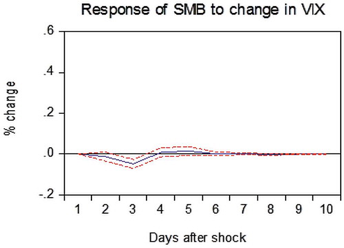
Impulse response function show the response of a variable to shock in another variable.¹ Figure 1 to 8 show the response of factors to one standard deviation innovation in the measure of investors’ sentiment. Figure 1 depicts that increase in D_VIX decreases SMB up to 3 days, but a change in D_GSVIs does not have a significant effect on SMB. The negative effect of D_VIX on SMB shows that following increases in VIX, small stocks underperform. The same is true for the period when the market is expected to go down (D_Crash and D_Bear), but in our findings, D_Crash has an insignificant relationship with SMB. The results of VAR and impulse response function show that the relationship between pricing factors and sentiment indices is mostly same as defined in explanation of hypothesis but not for all lags. The expected relationship of VIX and pessimistic GSVIs with size, value and market factor is negative, while it is positive for investment and profitability and vice versa for optimistic GSVIs.

Figure 1. Impulse response function for the Fama and French (2015) five-factors, Hou et al. (2015) q-factors, VIX and GSVIs.

Variance decomposition determines that how much of the forecast error variance of each of the factor can be explained by exogenous shocks to the other factor. The variance decomposition of factors and D_VIX is reported in Table 6.

Table 6. Variance decomposition of Fama–French’s five factor, q-factors and D_VIX

Period	S.E.	D_VIX	SMB	HML	CMA	RMW	RM-RF	ROE	IA	ME
Variance Decomposition of change in VIX
1	1.76	100.00	0.00	0.00	0.00	0.00	0.00	0.00	0.00	0.00
2	1.79	99.07	0.54	0.00	0.19	0.01	0.06	0.00	0.04	0.10
3	1.80	98.68	0.66	0.00	0.33	0.06	0.07	0.00	0.06	0.13
4	1.81	97.87	0.97	0.07	0.36	0.23	0.31	0.01	0.06	0.13
5	1.81	97.65	0.96	0.07	0.35	0.24	0.35	0.07	0.13	0.18
6	1.81	97.62	0.96	0.07	0.36	0.24	0.37	0.07	0.13	0.18
7	1.81	97.61	0.96	0.07	0.36	0.24	0.37	0.07	0.13	0.18
8	1.81	97.59	0.96	0.07	0.36	0.24	0.38	0.07	0.14	0.18
9	1.81	97.59	0.96	0.08	0.36	0.24	0.38	0.07	0.14	0.18
10	1.81	97.58	0.96	0.08	0.36	0.24	0.38	0.07	0.14	0.18
Variance Decomposition of SMB
1	0.58	4.48	95.52	0.00	0.00	0.00	0.00	0.00	0.00	0.00
2	0.58	4.46	95.42	0.01	0.00	0.00	0.06	0.01	0.01	0.02
3	0.58	4.82	94.77	0.06	0.03	0.07	0.17	0.04	0.02	0.03
4	0.58	4.80	94.12	0.19	0.16	0.11	0.18	0.16	0.02	0.27
5	0.59	4.84	93.59	0.24	0.18	0.46	0.18	0.16	0.06	0.29
6	0.59	4.84	93.58	0.24	0.18	0.46	0.19	0.16	0.06	0.30
7	0.59	4.84	93.56	0.25	0.18	0.46	0.19	0.16	0.06	0.30
8	0.59	4.84	93.55	0.25	0.18	0.46	0.19	0.16	0.06	0.30
9	0.59	4.84	93.55	0.25	0.18	0.46	0.19	0.16	0.07	0.30
10	0.59	4.84	93.55	0.25	0.18	0.46	0.19	0.16	0.07	0.30
Variance Decomposition of HML
1	0.57	8.61	0.12	91.26	0.00	0.00	0.00	0.00	0.00	0.00
2	0.57	8.60	0.13	90.99	0.13	0.01	0.00	0.00	0.13	0.00
3	0.57	8.63	0.26	90.49	0.36	0.03	0.01	0.00	0.17	0.05
4	0.57	8.61	0.30	90.28	0.40	0.03	0.04	0.02	0.23	0.08
5	0.58	8.49	0.34	88.97	0.42	0.27	1.10	0.09	0.24	0.08
6	0.58	8.49	0.35	88.95	0.43	0.27	1.10	0.09	0.24	0.08
7	0.58	8.49	0.35	88.94	0.43	0.27	1.10	0.09	0.24	0.08
8	0.58	8.51	0.36	88.91	0.44	0.27	1.10	0.09	0.24	0.08
9	0.58	8.51	0.36	88.89	0.44	0.27	1.10	0.10	0.24	0.08
10	0.58	8.51	0.36	88.89	0.44	0.27	1.10	0.10	0.24	0.08
Variance Decomposition of CMA
1	0.28	0.75	0.20	2.96	96.08	0.00	0.00	0.00	0.00	0.00
2	0.28	1.30	0.22	2.98	95.24	0.09	0.16	0.00	0.00	0.00
3	0.29	1.42	0.27	2.96	94.82	0.11	0.16	0.20	0.01	0.06
4	0.29	1.42	0.28	2.99	94.55	0.12	0.22	0.20	0.16	0.06
5	0.29	1.70	0.30	3.31	93.49	0.11	0.22	0.24	0.24	0.39
6	0.29	1.71	0.30	3.31	93.46	0.11	0.23	0.24	0.24	0.39
7	0.29	1.72	0.30	3.31	93.44	0.11	0.23	0.24	0.24	0.40
8	0.29	1.72	0.30	3.32	93.43	0.11	0.24	0.24	0.24	0.40
9	0.29	1.72	0.30	3.32	93.42	0.12	0.24	0.24	0.24	0.40
10	0.29	1.72	0.30	3.32	93.42	0.12	0.24	0.24	0.24	0.40
Variance Decomposition of RMW
1	0.34	11.36	8.05	6.99	1.78	71.81	0.00	0.00	0.00	0.00
2	0.34	11.44	8.06	7.04	1.86	71.26	0.18	0.01	0.14	0.01
3	0.35	11.47	8.20	6.98	2.11	70.60	0.20	0.06	0.14	0.24
4	0.35	11.51	8.19	6.96	2.19	70.28	0.23	0.10	0.29	0.26
5	0.35	11.45	8.12	7.07	2.19	69.50	0.82	0.12	0.45	0.28
6	0.35	11.47	8.11	7.06	2.21	69.46	0.82	0.12	0.45	0.28
7	0.35	11.49	8.11	7.06	2.22	69.44	0.82	0.12	0.45	0.29
8	0.35	11.49	8.12	7.06	2.22	69.42	0.82	0.12	0.45	0.29
9	0.35	11.49	8.12	7.06	2.22	69.42	0.83	0.12	0.45	0.29
10	0.35	11.49	8.12	7.06	2.22	69.41	0.83	0.12	0.45	0.29
Variance Decomposition of Rm-Rf
1	1.23	70.07	2.83	2.23	0.52	0.43	23.92	0.00	0.00	0.00
2	1.24	69.69	3.24	2.18	0.85	0.44	23.37	0.00	0.06	0.18
3	1.25	69.56	3.35	2.17	0.92	0.43	23.20	0.00	0.07	0.30
4	1.26	68.54	3.89	2.25	1.12	0.62	23.20	0.02	0.07	0.30
5	1.26	68.43	3.94	2.26	1.15	0.64	23.15	0.04	0.09	0.30
6	1.26	68.40	3.94	2.27	1.15	0.64	23.16	0.04	0.10	0.31
7	1.26	68.38	3.96	2.27	1.15	0.64	23.15	0.04	0.10	0.31
8	1.26	68.37	3.96	2.27	1.15	0.64	23.15	0.04	0.10	0.31
9	1.26	68.37	3.96	2.27	1.15	0.64	23.15	0.04	0.10	0.31
10	1.26	68.37	3.96	2.27	1.15	0.64	23.15	0.04	0.10	0.31
Variance Decomposition of ROE
1	0.41	8.86	7.27	16.71	0.05	12.27	0.54	54.31	0.00	0.00
2	0.41	9.65	7.29	16.49	0.15	12.03	0.85	53.41	0.03	0.10
3	0.41	9.67	7.27	16.43	0.18	11.99	0.97	53.30	0.03	0.15
4	0.41	9.64	7.24	16.43	0.18	11.94	1.20	53.11	0.09	0.16
5	0.42	9.56	7.17	16.24	0.27	11.87	2.11	52.50	0.12	0.16
6	0.42	9.57	7.16	16.23	0.30	11.87	2.11	52.47	0.12	0.16
7	0.42	9.57	7.16	16.23	0.30	11.87	2.11	52.47	0.12	0.16
8	0.42	9.58	7.17	16.23	0.30	11.87	2.11	52.45	0.12	0.16
9	0.42	9.58	7.17	16.22	0.30	11.87	2.12	52.45	0.12	0.16
10	0.42	9.58	7.17	16.22	0.30	11.87	2.12	52.45	0.12	0.17
Variance Decomposition of IA
1	0.29	0.32	0.02	6.54	65.97	0.16	0.03	0.77	26.19	0.00
2	0.29	0.48	0.07	6.62	65.63	0.19	0.09	0.78	26.10	0.03
3	0.30	0.56	0.11	6.59	65.47	0.19	0.09	0.94	25.96	0.09
4	0.30	0.57	0.18	6.59	65.37	0.20	0.10	0.96	25.94	0.09
5	0.30	0.79	0.29	7.01	64.47	0.23	0.19	0.97	25.66	0.39
6	0.30	0.80	0.29	7.01	64.45	0.23	0.20	0.98	25.66	0.40
7	0.30	0.80	0.29	7.01	64.44	0.23	0.20	0.98	25.65	0.40
8	0.30	0.80	0.29	7.01	64.44	0.23	0.20	0.98	25.65	0.40
9	0.30	0.80	0.29	7.01	64.43	0.23	0.21	0.98	25.65	0.40
10	0.30	0.80	0.29	7.01	64.43	0.23	0.21	0.98	25.65	0.40
Variance Decomposition of ME
1	0.60	8.36	85.61	0.51	0.11	0.03	0.14	1.70	0.08	3.46
2	0.60	8.33	85.52	0.55	0.15	0.05	0.17	1.70	0.10	3.44
3	0.61	8.57	85.04	0.58	0.19	0.12	0.22	1.73	0.10	3.45
4	0.61	8.52	84.43	0.69	0.39	0.20	0.22	1.82	0.11	3.62
5	0.61	8.53	83.91	0.70	0.40	0.65	0.22	1.82	0.16	3.61
6	0.61	8.53	83.90	0.70	0.40	0.65	0.22	1.82	0.16	3.61
7	0.61	8.53	83.88	0.70	0.40	0.65	0.23	1.82	0.16	3.61
8	0.61	8.53	83.88	0.71	0.40	0.65	0.23	1.82	0.16	3.61
9	0.61	8.53	83.87	0.71	0.40	0.65	0.23	1.82	0.17	3.61
10	0.61	8.53	83.87	0.71	0.40	0.65	0.23	1.82	0.17	3.61

The table represents variance decomposition of the forecast error (s.e) of factors and D_VIX and pricing factors for the period of 10 days. These variables represent the variations in forecast error due to variations in each of the variable. “Period” shows the number of days aftershock, “s.e” shows the forecast error, and other columns show the amount of variation explained over the period of 10 days

Table 6 (Panel A) shows that variance in D_VIX is fully explained by itself in period 1. On average 3% of variance gets explained by other factors over the period of 2 to 10 days but D_VIX explains more variance in other factors. It determines approximately 4% variance in SMB, 8% in HML, 11% in RMW, 9% in ROE, 8% in ME and 68% in Rm-Rf (see Panel B to I of Table 6). D_VIX has significant contribution in determining the market risk premium (Rm-Rf), showing VIX is a better proxy for market sentiments as it moves more closely with the market.

As explained earlier, two competing asset pricing models in this study include the pricing factors which represent similar economic phenomenon but measured differently such as CMA and IA for investment, SMB and ME for size and RMW and ROE for profitability. The variance decomposition test helps us to distinguish the robust factors. ME explained approximately 3.5% own variance over 10 days period, and its 84% is explained by SMB but the opposite is not true. This indicates that SMB is superior to ME may be owing to different portfolio construction of these pricing factors. Similarly, the 65% of the variance of q-factor model based IA explained by CMA.

Then, the variance decomposition results for GSVIs and the prominent pricing factors included in this research are contained in Table 7-10. The results show that on whole, GSVIs contribute very little in explaining the variance of prominent pricing factors. It can be because GSVIs may not be related to risk factors directly or underlying attributes of these risk factors.

Table 7. Variance Decomposition of Fama–French’s five factor, q-factors and Market Crash

Period	S.E.	D_Crash	SMB	HML	CMA	RMW	Rm-Rf	ROE	IA	ME
Variance Decomposition of Market Crash
1	0.56	100.00	0.00	0.00	0.00	0.00	0.00	0.00	0.00	0.00
2	0.65	99.51	0.14	0.02	0.04	0.04	0.03	0.03	0.03	0.16
3	0.66	99.23	0.16	0.02	0.13	0.12	0.06	0.03	0.05	0.20
4	0.66	98.93	0.31	0.02	0.13	0.15	0.06	0.10	0.05	0.24
5	0.66	98.56	0.31	0.02	0.18	0.25	0.06	0.20	0.06	0.36
6	0.66	98.45	0.31	0.02	0.20	0.26	0.11	0.20	0.07	0.37
7	0.66	98.44	0.32	0.02	0.20	0.27	0.11	0.20	0.07	0.37
8	0.66	98.43	0.32	0.02	0.20	0.27	0.11	0.20	0.07	0.37
9	0.67	98.41	0.33	0.02	0.20	0.27	0.11	0.21	0.07	0.37
10	0.67	98.40	0.33	0.02	0.20	0.28	0.11	0.21	0.07	0.38
Variance Decomposition of SMB
1	0.58	0.01	99.99	0.00	0.00	0.00	0.00	0.00	0.00	0.00
2	0.58	0.01	99.94	0.00	0.00	0.00	0.00	0.01	0.02	0.02
3	0.58	0.17	98.89	0.17	0.06	0.14	0.46	0.03	0.02	0.05
4	0.58	0.34	98.06	0.29	0.18	0.19	0.46	0.16	0.02	0.30
5	0.59	0.34	97.54	0.32	0.21	0.59	0.47	0.16	0.06	0.31
6	0.59	0.35	97.52	0.32	0.21	0.59	0.48	0.16	0.06	0.32
7	0.59	0.35	97.50	0.32	0.21	0.59	0.48	0.16	0.06	0.32
8	0.59	0.36	97.48	0.32	0.21	0.59	0.48	0.16	0.06	0.32
9	0.59	0.36	97.48	0.33	0.21	0.59	0.48	0.16	0.07	0.32
10	0.59	0.36	97.48	0.33	0.21	0.59	0.48	0.16	0.07	0.32
Variance Decomposition of HML
1	0.57	0.80	0.87	98.33	0.00	0.00	0.00	0.00	0.00	0.00
2	0.57	0.80	0.87	98.06	0.11	0.01	0.01	0.00	0.13	0.01
3	0.57	0.95	1.05	97.33	0.34	0.03	0.05	0.00	0.17	0.08
4	0.57	1.16	1.06	96.90	0.39	0.04	0.09	0.03	0.24	0.09
5	0.58	1.45	1.09	95.86	0.40	0.25	0.48	0.13	0.25	0.09
6	0.58	1.58	1.10	95.69	0.41	0.25	0.49	0.13	0.25	0.09
7	0.58	1.58	1.10	95.68	0.41	0.26	0.49	0.13	0.25	0.10
8	0.58	1.59	1.10	95.66	0.41	0.26	0.49	0.13	0.25	0.10
9	0.58	1.59	1.11	95.65	0.41	0.26	0.49	0.13	0.26	0.10
10	0.58	1.60	1.11	95.64	0.41	0.26	0.49	0.13	0.26	0.10
Variance Decomposition of CMA
1	0.28	0.15	0.07	2.07	97.72	0.00	0.00	0.00	0.00	0.00
2	0.28	0.25	0.15	2.04	96.79	0.24	0.53	0.00	0.00	0.00
3	0.28	0.27	0.17	2.05	96.40	0.29	0.56	0.20	0.01	0.06
4	0.29	0.27	0.19	2.09	96.15	0.29	0.60	0.20	0.16	0.06
5	0.29	0.38	0.25	2.53	95.05	0.29	0.65	0.24	0.23	0.38
6	0.29	0.40	0.25	2.54	95.00	0.29	0.67	0.24	0.23	0.39
7	0.29	0.40	0.25	2.54	94.99	0.29	0.67	0.24	0.23	0.39
8	0.29	0.40	0.25	2.55	94.97	0.29	0.67	0.24	0.24	0.39
9	0.29	0.40	0.25	2.55	94.96	0.29	0.67	0.24	0.24	0.39
10	0.29	0.40	0.25	2.55	94.96	0.29	0.67	0.24	0.24	0.39
Variance Decomposition of RMW
1	0.34	0.86	12.02	10.30	1.23	75.59	0.00	0.00	0.00	0.00
2	0.34	0.86	12.05	10.26	1.37	75.05	0.25	0.02	0.14	0.00
3	0.34	0.91	12.22	10.15	1.65	74.28	0.27	0.08	0.15	0.30
4	0.35	1.07	12.16	10.10	1.70	73.96	0.27	0.12	0.32	0.30
5	0.35	1.28	12.01	10.05	1.69	72.99	1.06	0.15	0.45	0.31
6	0.35	1.40	11.99	10.04	1.70	72.87	1.08	0.15	0.45	0.32
7	0.35	1.40	11.99	10.04	1.72	72.84	1.08	0.15	0.45	0.33
8	0.35	1.40	11.99	10.04	1.72	72.83	1.09	0.15	0.46	0.33
9	0.35	1.40	11.99	10.04	1.72	72.82	1.10	0.15	0.46	0.33
10	0.35	1.41	11.99	10.04	1.72	72.82	1.10	0.15	0.46	0.33
Variance Decomposition of Rm-Rf
1	1.23	0.73	11.33	12.59	2.90	4.93	67.51	0.00	0.00	0.00
2	1.24	0.82	11.28	12.52	3.38	4.98	66.85	0.00	0.06	0.13
3	1.24	0.84	11.27	12.47	3.38	4.97	66.77	0.00	0.07	0.22
4	1.26	1.18	11.57	12.27	3.46	4.93	66.27	0.03	0.07	0.23
5	1.26	1.27	11.57	12.27	3.50	4.95	66.08	0.05	0.08	0.23
6	1.26	1.35	11.56	12.25	3.49	4.95	66.02	0.05	0.09	0.24
7	1.26	1.36	11.56	12.25	3.49	4.95	66.01	0.05	0.09	0.24
8	1.26	1.37	11.57	12.25	3.49	4.96	65.99	0.05	0.09	0.24
9	1.26	1.38	11.57	12.25	3.49	4.96	65.99	0.05	0.09	0.24
10	1.26	1.38	11.57	12.25	3.49	4.96	65.98	0.05	0.09	0.24
Variance Decomposition of ROE
1	0.41	0.51	10.52	20.78	0.14	13.28	0.38	54.38	0.00	0.00
2	0.41	0.52	10.67	20.69	0.34	13.01	1.24	53.40	0.03	0.09
3	0.41	0.52	10.63	20.62	0.38	12.97	1.42	53.25	0.04	0.18
4	0.42	0.72	10.57	20.58	0.38	12.91	1.51	53.03	0.11	0.19
5	0.42	0.73	10.51	20.42	0.44	12.85	2.07	52.65	0.13	0.19
6	0.42	0.78	10.50	20.41	0.47	12.86	2.08	52.59	0.13	0.19
7	0.42	0.78	10.50	20.41	0.47	12.86	2.08	52.58	0.13	0.19
8	0.42	0.78	10.50	20.41	0.48	12.86	2.08	52.58	0.13	0.19
9	0.42	0.78	10.50	20.40	0.48	12.86	2.09	52.57	0.13	0.19
10	0.42	0.78	10.50	20.40	0.48	12.86	2.09	52.57	0.13	0.19
Variance Decomposition of IA
1	0.29	0.01	0.00	5.41	67.37	0.18	0.01	0.74	26.29	0.00
2	0.29	0.13	0.09	5.42	66.98	0.26	0.18	0.75	26.15	0.03
3	0.30	0.13	0.10	5.39	66.86	0.28	0.22	0.92	26.01	0.09
4	0.30	0.14	0.19	5.40	66.75	0.28	0.23	0.93	25.99	0.09
5	0.30	0.19	0.36	5.94	65.82	0.30	0.33	0.94	25.72	0.39
6	0.30	0.20	0.36	5.94	65.80	0.30	0.35	0.95	25.71	0.40
7	0.30	0.20	0.36	5.94	65.79	0.30	0.35	0.95	25.70	0.40
8	0.30	0.20	0.36	5.94	65.79	0.30	0.35	0.95	25.70	0.40
9	0.30	0.20	0.36	5.94	65.78	0.31	0.36	0.95	25.70	0.40
10	0.30	0.20	0.36	5.94	65.78	0.31	0.36	0.95	25.70	0.40
Variance Decomposition of ME
1	0.60	0.00	93.27	0.83	0.16	0.10	0.42	1.70	0.08	3.44
2	0.60	0.00	93.19	0.85	0.18	0.13	0.42	1.69	0.11	3.43
3	0.60	0.26	92.34	0.96	0.25	0.25	0.68	1.71	0.11	3.44
4	0.61	0.35	91.58	1.06	0.45	0.33	0.68	1.80	0.12	3.63
5	0.61	0.39	91.02	1.06	0.47	0.80	0.67	1.81	0.17	3.61
6	0.61	0.40	91.01	1.06	0.47	0.80	0.68	1.81	0.17	3.61
7	0.61	0.40	90.99	1.06	0.47	0.80	0.68	1.81	0.17	3.61
8	0.61	0.42	90.97	1.07	0.47	0.80	0.68	1.81	0.17	3.61
9	0.61	0.42	90.96	1.07	0.47	0.80	0.68	1.81	0.17	3.61
10	0.61	0.42	90.96	1.07	0.47	0.80	0.68	1.81	0.17	3.61

The table represents variance decomposition of the forecast error (s.e) of factors and D_Crash and pricing factors for the period of 10 days. These variables represent the variations in forecast error due to variations in each of the variable. “Period” shows the number of days aftershock, “s.e” shows the forecast error, and other columns show the amount of variation explained over the period of 10 days

Table 8. Variance decomposition of Fama–French’s five factor, q-factors and Bear Market

Period	S.E.	D_Bear	SMB	HML	CMA	RMW	Rm-Rf	ROE	IA	ME
Variance Decomposition of Bear Market
1	0.51	100.00	0.00	0.00	0.00	0.00	0.00	0.00	0.00	0.00
2	0.61	99.54	0.02	0.21	0.00	0.01	0.03	0.00	0.13	0.05
3	0.61	99.30	0.04	0.26	0.03	0.05	0.04	0.00	0.19	0.09
4	0.61	99.06	0.05	0.27	0.03	0.06	0.05	0.08	0.20	0.20
5	0.61	98.81	0.05	0.28	0.04	0.17	0.10	0.12	0.24	0.20
6	0.61	98.72	0.06	0.28	0.04	0.19	0.15	0.12	0.25	0.21
7	0.62	98.71	0.06	0.28	0.04	0.19	0.15	0.12	0.25	0.21
8	0.62	98.70	0.06	0.28	0.04	0.19	0.15	0.12	0.25	0.21
9	0.62	98.69	0.06	0.28	0.04	0.19	0.15	0.12	0.25	0.21
10	0.62	98.69	0.06	0.28	0.04	0.20	0.15	0.12	0.25	0.21
Variance Decomposition of SMB
1	0.58	0.07	99.93	0.00	0.00	0.00	0.00	0.00	0.00	0.00
2	0.58	0.13	99.83	0.00	0.00	0.00	0.00	0.01	0.02	0.01
3	0.58	0.15	98.92	0.19	0.07	0.16	0.42	0.04	0.02	0.03
4	0.58	0.16	98.25	0.29	0.21	0.22	0.42	0.16	0.02	0.28
5	0.59	0.20	97.65	0.31	0.24	0.63	0.44	0.16	0.06	0.29
6	0.59	0.22	97.62	0.31	0.24	0.63	0.45	0.16	0.06	0.30
7	0.59	0.22	97.61	0.32	0.24	0.63	0.45	0.16	0.07	0.30
8	0.59	0.22	97.60	0.32	0.24	0.64	0.45	0.16	0.07	0.30
9	0.59	0.22	97.59	0.32	0.24	0.64	0.45	0.16	0.07	0.30
10	0.59	0.23	97.59	0.32	0.24	0.64	0.45	0.16	0.07	0.30
Variance Decomposition of HML
1	0.57	0.00	0.91	99.09	0.00	0.00	0.00	0.00	0.00	0.00
2	0.57	0.04	0.91	98.78	0.13	0.01	0.00	0.00	0.12	0.00
3	0.57	0.04	1.06	98.26	0.37	0.02	0.04	0.00	0.16	0.05
4	0.58	0.09	1.08	98.00	0.41	0.03	0.07	0.02	0.22	0.07
5	0.58	0.13	1.11	97.18	0.44	0.29	0.42	0.12	0.23	0.08
6	0.58	0.14	1.12	97.15	0.45	0.29	0.43	0.13	0.23	0.08
7	0.58	0.14	1.12	97.14	0.45	0.29	0.43	0.13	0.23	0.08
8	0.58	0.14	1.12	97.13	0.45	0.29	0.43	0.13	0.23	0.08
9	0.58	0.14	1.12	97.12	0.45	0.29	0.44	0.13	0.24	0.08
10	0.58	0.14	1.12	97.12	0.45	0.29	0.44	0.13	0.24	0.08
Variance Decomposition of CMA
1	0.28	0.00	0.07	1.93	98.01	0.00	0.00	0.00	0.00	0.00
2	0.28	0.06	0.16	1.90	97.05	0.22	0.59	0.00	0.00	0.00
3	0.28	0.06	0.18	1.91	96.68	0.27	0.61	0.22	0.01	0.06
4	0.29	0.13	0.20	1.95	96.35	0.27	0.65	0.22	0.18	0.06
5	0.29	0.13	0.25	2.43	95.29	0.27	0.70	0.26	0.26	0.40
6	0.29	0.19	0.25	2.44	95.20	0.27	0.72	0.26	0.26	0.41
7	0.29	0.19	0.25	2.45	95.19	0.27	0.72	0.26	0.26	0.41
8	0.29	0.19	0.25	2.45	95.18	0.27	0.72	0.26	0.27	0.41
9	0.29	0.19	0.25	2.45	95.16	0.27	0.73	0.26	0.27	0.41
10	0.29	0.19	0.25	2.45	95.16	0.27	0.73	0.26	0.27	0.41
Variance Decomposition of RMW
1	0.34	0.13	12.05	11.02	1.10	75.70	0.00	0.00	0.00	0.00
2	0.34	0.13	12.09	10.98	1.22	75.16	0.25	0.01	0.15	0.01
3	0.35	0.17	12.24	10.87	1.51	74.48	0.26	0.06	0.15	0.26
4	0.35	0.17	12.19	10.83	1.57	74.28	0.28	0.10	0.31	0.28
5	0.35	0.17	12.07	10.82	1.56	73.46	1.07	0.13	0.45	0.29
6	0.35	0.17	12.06	10.81	1.58	73.42	1.09	0.13	0.45	0.29
7	0.35	0.17	12.06	10.82	1.60	73.39	1.10	0.13	0.45	0.29
8	0.35	0.17	12.06	10.81	1.60	73.38	1.11	0.13	0.45	0.29
9	0.35	0.17	12.06	10.81	1.60	73.37	1.11	0.13	0.45	0.29
10	0.35	0.17	12.06	10.81	1.60	73.37	1.11	0.13	0.45	0.29
Variance Decomposition of Rm-Rf
1	1.23	1.04	11.31	13.31	2.99	4.89	66.46	0.00	0.00	0.00
2	1.24	1.09	11.25	13.20	3.47	4.92	65.82	0.01	0.06	0.18
3	1.25	1.09	11.23	13.16	3.48	4.90	65.75	0.01	0.07	0.31
4	1.26	1.11	11.54	13.01	3.57	4.91	65.45	0.03	0.07	0.31
5	1.26	1.12	11.54	13.02	3.62	4.95	65.30	0.05	0.09	0.31
6	1.26	1.12	11.54	13.02	3.61	4.94	65.30	0.05	0.09	0.32
7	1.26	1.13	11.55	13.01	3.61	4.94	65.29	0.05	0.10	0.32
8	1.26	1.13	11.55	13.01	3.61	4.95	65.28	0.05	0.10	0.32
9	1.26	1.13	11.55	13.01	3.61	4.95	65.28	0.05	0.10	0.32
10	1.26	1.13	11.55	13.01	3.61	4.95	65.28	0.05	0.10	0.32
Variance Decomposition of ROE
1	0.41	0.02	10.63	21.26	0.15	13.34	0.42	54.20	0.00	0.00
2	0.41	0.03	10.77	21.15	0.34	13.07	1.24	53.29	0.02	0.08
3	0.41	0.11	10.73	21.07	0.37	13.03	1.38	53.13	0.03	0.13
4	0.42	0.13	10.70	21.09	0.37	12.99	1.47	53.00	0.10	0.14
5	0.42	0.13	10.64	20.93	0.44	12.94	2.03	52.63	0.12	0.14
6	0.42	0.13	10.63	20.92	0.47	12.95	2.05	52.59	0.12	0.14
7	0.42	0.13	10.63	20.92	0.47	12.95	2.05	52.58	0.12	0.14
8	0.42	0.13	10.63	20.92	0.48	12.95	2.05	52.57	0.12	0.14
9	0.42	0.14	10.63	20.92	0.48	12.95	2.06	52.57	0.12	0.14
10	0.42	0.14	10.63	20.92	0.48	12.95	2.06	52.57	0.12	0.14
Variance Decomposition of IA
1	0.29	0.03	0.00	5.36	67.44	0.18	0.00	0.73	26.27	0.00
2	0.29	0.24	0.10	5.37	66.93	0.25	0.22	0.75	26.10	0.04
3	0.29	0.27	0.12	5.35	66.78	0.27	0.25	0.93	25.95	0.09
4	0.30	0.35	0.20	5.35	66.62	0.27	0.26	0.94	25.92	0.09
5	0.30	0.37	0.36	5.91	65.68	0.29	0.36	0.96	25.64	0.42
6	0.30	0.42	0.36	5.92	65.63	0.29	0.38	0.97	25.62	0.42
7	0.30	0.42	0.36	5.92	65.62	0.29	0.38	0.97	25.62	0.43
8	0.30	0.42	0.36	5.92	65.62	0.29	0.38	0.97	25.62	0.43
9	0.30	0.43	0.36	5.92	65.61	0.29	0.38	0.97	25.61	0.43
10	0.30	0.43	0.36	5.92	65.61	0.29	0.38	0.97	25.61	0.43
Variance Decomposition of ME
1	0.60	0.15	93.09	0.86	0.17	0.09	0.39	1.70	0.08	3.47
2	0.60	0.18	92.98	0.87	0.19	0.12	0.40	1.70	0.11	3.45
3	0.60	0.19	92.32	1.01	0.28	0.27	0.64	1.73	0.11	3.46
4	0.61	0.20	91.66	1.09	0.48	0.36	0.64	1.82	0.11	3.64
5	0.61	0.25	91.05	1.09	0.51	0.86	0.64	1.83	0.16	3.62
6	0.61	0.27	91.02	1.08	0.51	0.86	0.64	1.83	0.16	3.63
7	0.61	0.27	91.01	1.09	0.51	0.86	0.64	1.83	0.16	3.63
8	0.61	0.27	91.00	1.09	0.51	0.86	0.64	1.83	0.16	3.63
9	0.61	0.27	91.00	1.10	0.51	0.86	0.64	1.83	0.16	3.63
10	0.61	0.27	91.00	1.10	0.51	0.86	0.64	1.83	0.16	3.63

The table represents variance decomposition of the forecast error (s.e) of factors and D_Bear and pricing factors for the period of 10 days. These variables represent the variations in forecast error due to variations in each of the variable. “Period” shows the number of days aftershock, “s.e” shows the forecast error, and other columns show the amount of variation explained over the period of 10 days

Table 9. Variance decomposition of Fama–French’s five factor, q-factors and Bull Market

Period	S.E.	D_Bull	SMB	HML	CMA	RMW	Rm-Rf	ROE	IA	ME
Variance Decomposition of Bull Market
1	0.54	100.00	0.00	0.00	0.00	0.00	0.00	0.00	0.00	0.00
2	0.63	99.96	0.00	0.00	0.01	0.00	0.00	0.00	0.03	0.00
3	0.63	99.73	0.05	0.00	0.03	0.08	0.01	0.01	0.08	0.01
4	0.63	99.54	0.07	0.01	0.06	0.12	0.02	0.08	0.09	0.02
5	0.63	99.46	0.12	0.01	0.06	0.12	0.02	0.08	0.09	0.03
6	0.64	99.39	0.15	0.01	0.07	0.12	0.03	0.08	0.10	0.05
7	0.64	99.39	0.15	0.01	0.07	0.12	0.03	0.08	0.10	0.05
8	0.64	99.39	0.15	0.01	0.07	0.12	0.03	0.08	0.10	0.05
9	0.64	99.38	0.15	0.01	0.07	0.12	0.03	0.09	0.10	0.05
10	0.64	99.38	0.15	0.01	0.07	0.12	0.03	0.09	0.10	0.05
Variance Decomposition of SMB
1	0.58	0.00	100.00	0.00	0.00	0.00	0.00	0.00	0.00	0.00
2	0.58	0.02	99.94	0.00	0.00	0.00	0.00	0.01	0.02	0.01
3	0.58	0.04	99.01	0.19	0.07	0.16	0.44	0.04	0.02	0.03
4	0.58	0.05	98.35	0.29	0.21	0.22	0.43	0.16	0.02	0.27
5	0.59	0.06	97.81	0.31	0.24	0.62	0.45	0.17	0.06	0.28
6	0.59	0.07	97.79	0.31	0.24	0.62	0.45	0.17	0.06	0.29
7	0.59	0.07	97.77	0.32	0.24	0.63	0.46	0.17	0.07	0.29
8	0.59	0.07	97.76	0.32	0.24	0.63	0.46	0.17	0.07	0.29
9	0.59	0.07	97.76	0.32	0.24	0.63	0.46	0.17	0.07	0.29
10	0.59	0.07	97.76	0.32	0.24	0.63	0.46	0.17	0.07	0.29
Variance Decomposition of HML
1	0.57	0.00	0.91	99.08	0.00	0.00	0.00	0.00	0.00	0.00
2	0.57	0.09	0.91	98.74	0.13	0.01	0.00	0.00	0.11	0.00
3	0.57	0.09	1.06	98.22	0.36	0.02	0.04	0.00	0.15	0.06
4	0.58	0.21	1.08	97.91	0.40	0.02	0.06	0.02	0.21	0.08
5	0.58	0.23	1.11	97.09	0.43	0.27	0.44	0.13	0.22	0.09
6	0.58	0.24	1.12	97.05	0.44	0.27	0.44	0.13	0.22	0.09
7	0.58	0.24	1.12	97.04	0.44	0.27	0.44	0.13	0.22	0.09
8	0.58	0.24	1.12	97.03	0.44	0.27	0.45	0.13	0.22	0.09
9	0.58	0.25	1.13	97.02	0.44	0.27	0.45	0.13	0.22	0.09
10	0.58	0.25	1.13	97.02	0.44	0.28	0.45	0.13	0.22	0.09
Variance Decomposition of CMA
1	0.28	0.13	0.07	1.90	97.91	0.00	0.00	0.00	0.00	0.00
2	0.28	0.21	0.16	1.88	97.00	0.20	0.55	0.00	0.00	0.00
3	0.29	0.24	0.17	1.89	96.61	0.25	0.57	0.21	0.01	0.06
4	0.29	0.24	0.19	1.92	96.37	0.25	0.60	0.21	0.16	0.06
5	0.29	0.24	0.25	2.41	95.34	0.25	0.66	0.24	0.23	0.38
6	0.29	0.26	0.25	2.41	95.28	0.25	0.68	0.25	0.23	0.38
7	0.29	0.26	0.25	2.42	95.27	0.25	0.68	0.25	0.24	0.39
8	0.29	0.26	0.25	2.43	95.26	0.25	0.68	0.25	0.24	0.39
9	0.29	0.26	0.25	2.43	95.25	0.25	0.68	0.25	0.24	0.39
10	0.29	0.26	0.25	2.43	95.25	0.25	0.68	0.25	0.24	0.39
Variance Decomposition of RMW
1	0.34	0.06	12.06	11.00	1.09	75.80	0.00	0.00	0.00	0.00
2	0.34	0.06	12.10	10.95	1.22	75.25	0.27	0.01	0.14	0.01
3	0.35	0.22	12.24	10.83	1.49	74.48	0.28	0.05	0.14	0.26
4	0.35	0.23	12.19	10.78	1.55	74.26	0.29	0.10	0.31	0.28
5	0.35	0.24	12.06	10.77	1.55	73.44	1.07	0.13	0.44	0.29
6	0.35	0.27	12.06	10.77	1.57	73.39	1.09	0.13	0.45	0.29
7	0.35	0.27	12.05	10.77	1.58	73.36	1.10	0.13	0.45	0.29
8	0.35	0.27	12.06	10.77	1.58	73.35	1.11	0.13	0.45	0.29
9	0.35	0.27	12.06	10.77	1.58	73.34	1.12	0.13	0.45	0.29
10	0.35	0.27	12.06	10.77	1.58	73.34	1.12	0.13	0.45	0.30
Variance Decomposition of Rm-Rf
1	1.23	0.04	11.40	13.22	2.92	5.04	67.38	0.00	0.00	0.00
2	1.24	0.06	11.37	13.13	3.39	5.06	66.75	0.01	0.05	0.18
3	1.25	0.09	11.34	13.09	3.40	5.04	66.67	0.01	0.06	0.31
4	1.26	0.13	11.66	12.93	3.50	5.06	66.33	0.03	0.06	0.31
5	1.26	0.14	11.67	12.94	3.54	5.09	66.19	0.05	0.07	0.31
6	1.26	0.14	11.67	12.94	3.54	5.08	66.18	0.05	0.08	0.32
7	1.26	0.14	11.68	12.94	3.54	5.08	66.17	0.05	0.08	0.32
8	1.26	0.14	11.68	12.94	3.54	5.09	66.17	0.05	0.08	0.32
9	1.26	0.14	11.68	12.94	3.54	5.09	66.16	0.05	0.08	0.32
10	1.26	0.14	11.68	12.94	3.54	5.09	66.16	0.05	0.08	0.32
Variance Decomposition of ROE
1	0.41	0.04	10.56	21.19	0.14	13.34	0.39	54.33	0.00	0.00
2	0.41	0.10	10.69	21.07	0.34	13.06	1.27	53.36	0.03	0.08
3	0.41	0.10	10.66	21.00	0.38	13.03	1.42	53.23	0.04	0.14
4	0.42	0.11	10.63	21.02	0.38	12.99	1.51	53.13	0.10	0.15
5	0.42	0.13	10.56	20.86	0.45	12.93	2.06	52.74	0.12	0.15
6	0.42	0.13	10.56	20.85	0.48	12.94	2.07	52.70	0.12	0.15
7	0.42	0.13	10.56	20.85	0.48	12.94	2.08	52.70	0.12	0.15
8	0.42	0.13	10.56	20.85	0.48	12.94	2.08	52.69	0.12	0.15
9	0.42	0.13	10.56	20.85	0.48	12.94	2.08	52.69	0.12	0.15
10	0.42	0.13	10.56	20.85	0.48	12.94	2.08	52.69	0.12	0.15
Variance Decomposition of IA
1	0.29	0.09	0.00	5.31	67.42	0.18	0.01	0.73	26.27	0.00
2	0.29	0.22	0.09	5.33	67.02	0.23	0.19	0.74	26.14	0.03
3	0.30	0.31	0.10	5.30	66.83	0.26	0.22	0.91	25.98	0.09
4	0.30	0.33	0.18	5.30	66.72	0.26	0.23	0.92	25.96	0.09
5	0.30	0.34	0.36	5.87	65.80	0.28	0.34	0.94	25.68	0.40
6	0.30	0.35	0.36	5.88	65.77	0.28	0.36	0.94	25.67	0.40
7	0.30	0.35	0.36	5.88	65.77	0.28	0.36	0.94	25.67	0.40
8	0.30	0.35	0.36	5.88	65.76	0.28	0.36	0.94	25.67	0.41
9	0.30	0.35	0.36	5.88	65.75	0.28	0.36	0.94	25.67	0.41
10	0.30	0.35	0.36	5.88	65.75	0.28	0.36	0.94	25.67	0.41
Variance Decomposition of ME
1	0.60	0.00	93.22	0.86	0.17	0.10	0.40	1.70	0.08	3.46
2	0.60	0.02	93.13	0.87	0.19	0.12	0.41	1.70	0.11	3.45
3	0.61	0.05	92.45	1.01	0.28	0.27	0.66	1.73	0.11	3.45
4	0.61	0.05	91.78	1.09	0.48	0.37	0.66	1.82	0.12	3.63
5	0.61	0.07	91.22	1.08	0.51	0.85	0.66	1.83	0.17	3.61
6	0.61	0.08	91.21	1.08	0.51	0.85	0.66	1.83	0.17	3.62
7	0.61	0.08	91.19	1.09	0.51	0.86	0.66	1.83	0.17	3.62
8	0.61	0.08	91.18	1.09	0.51	0.86	0.66	1.83	0.17	3.62
9	0.61	0.08	91.18	1.09	0.51	0.86	0.66	1.83	0.17	3.62
10	0.61	0.08	91.17	1.09	0.51	0.86	0.66	1.83	0.17	3.62

The table represents variance decomposition of the forecast error (s.e) of factors and D_Bull and pricing factors for the period of 10 days. These variables represent the variations in forecast error due to variations in each of the variable. “Period” shows the number of days aftershock, “s.e” shows the forecast error, and other columns show the amount of variation explained over the period of 10 days

Table 10. Variance Decomposition of Fama–French’s five factor, q-factors and Market Rally

Period	S.E.	D_Rally	SMB	HML	CMA	RMW	Rm-Rf	ROE	IA	ME
Variance Decomposition of Market Rally
1	0.99	100.00	0.00	0.00	0.00	0.00	0.00	0.00	0.00	0.00
2	1.09	99.79	0.02	0.08	0.00	0.03	0.01	0.04	0.00	0.01
3	1.10	99.73	0.03	0.09	0.02	0.04	0.02	0.05	0.00	0.01
4	1.11	99.07	0.11	0.14	0.23	0.05	0.03	0.33	0.02	0.02
5	1.11	98.86	0.11	0.18	0.27	0.14	0.03	0.37	0.02	0.02
6	1.12	98.80	0.12	0.21	0.28	0.14	0.03	0.36	0.03	0.03
7	1.12	98.78	0.12	0.20	0.29	0.14	0.03	0.36	0.03	0.03
8	1.12	98.77	0.12	0.21	0.30	0.14	0.04	0.36	0.03	0.03
9	1.12	98.75	0.12	0.21	0.30	0.14	0.04	0.37	0.04	0.03
10	1.12	98.75	0.12	0.21	0.30	0.14	0.04	0.37	0.04	0.03
Variance Decomposition of SMB
1	0.58	0.00	100.00	0.00	0.00	0.00	0.00	0.00	0.00	0.00
2	0.58	0.01	99.95	0.00	0.00	0.00	0.00	0.01	0.02	0.01
3	0.58	0.01	99.04	0.19	0.07	0.17	0.43	0.04	0.02	0.03
4	0.58	0.12	98.27	0.29	0.22	0.23	0.43	0.17	0.02	0.26
5	0.59	0.15	97.71	0.31	0.25	0.64	0.44	0.17	0.06	0.28
6	0.59	0.15	97.69	0.31	0.25	0.64	0.45	0.17	0.06	0.28
7	0.59	0.15	97.67	0.32	0.25	0.64	0.45	0.17	0.06	0.28
8	0.59	0.15	97.67	0.32	0.25	0.64	0.45	0.17	0.06	0.28
9	0.59	0.15	97.66	0.32	0.25	0.64	0.45	0.17	0.07	0.28
10	0.59	0.15	97.66	0.32	0.25	0.64	0.45	0.17	0.07	0.28
Variance Decomposition of HML
1	0.57	0.08	0.92	99.00	0.00	0.00	0.00	0.00	0.00	0.00
2	0.57	0.10	0.92	98.71	0.14	0.01	0.00	0.00	0.12	0.00
3	0.58	0.11	1.07	98.17	0.38	0.02	0.04	0.00	0.16	0.05
4	0.58	0.11	1.10	97.96	0.43	0.03	0.06	0.02	0.22	0.08
5	0.58	0.11	1.13	97.16	0.45	0.28	0.44	0.13	0.23	0.08
6	0.58	0.11	1.13	97.13	0.46	0.28	0.45	0.13	0.23	0.08
7	0.58	0.11	1.14	97.12	0.46	0.28	0.45	0.13	0.23	0.08
8	0.58	0.12	1.14	97.11	0.46	0.28	0.45	0.13	0.23	0.08
9	0.58	0.12	1.14	97.10	0.46	0.28	0.46	0.13	0.24	0.08
10	0.58	0.12	1.14	97.10	0.46	0.28	0.46	0.13	0.24	0.08
Variance Decomposition of CMA
1	0.28	0.00	0.07	1.87	98.07	0.00	0.00	0.00	0.00	0.00
2	0.28	0.00	0.16	1.85	97.24	0.21	0.54	0.00	0.00	0.00
3	0.29	0.06	0.17	1.86	96.82	0.25	0.57	0.20	0.01	0.06
4	0.29	0.08	0.19	1.90	96.55	0.25	0.60	0.20	0.17	0.06
5	0.29	0.10	0.25	2.39	95.50	0.26	0.65	0.24	0.24	0.37
6	0.29	0.10	0.25	2.39	95.46	0.26	0.67	0.25	0.24	0.37
7	0.29	0.10	0.25	2.40	95.45	0.26	0.67	0.25	0.24	0.38
8	0.29	0.11	0.25	2.40	95.43	0.26	0.67	0.25	0.25	0.38
9	0.29	0.11	0.25	2.40	95.42	0.26	0.68	0.25	0.25	0.38
10	0.29	0.11	0.25	2.40	95.42	0.26	0.68	0.25	0.25	0.38
Variance Decomposition of RMW
1	0.34	0.00	12.19	10.98	1.12	75.72	0.00	0.00	0.00	0.00
2	0.34	0.01	12.21	10.93	1.23	75.18	0.26	0.01	0.15	0.01
3	0.35	0.03	12.37	10.83	1.53	74.50	0.28	0.06	0.16	0.26
4	0.35	0.05	12.32	10.78	1.59	74.27	0.30	0.10	0.32	0.28
5	0.35	0.11	12.18	10.77	1.58	73.41	1.08	0.13	0.46	0.29
6	0.35	0.11	12.18	10.76	1.60	73.37	1.09	0.13	0.46	0.29
7	0.35	0.11	12.17	10.77	1.61	73.34	1.11	0.13	0.46	0.29
8	0.35	0.11	12.18	10.76	1.61	73.33	1.11	0.13	0.46	0.29
9	0.35	0.12	12.18	10.76	1.61	73.32	1.12	0.13	0.46	0.29
10	0.35	0.12	12.18	10.76	1.61	73.32	1.12	0.13	0.46	0.29
Variance Decomposition of Rm-Rf
1	1.23	0.00	11.42	13.25	2.93	5.07	67.33	0.00	0.00	0.00
2	1.24	0.01	11.38	13.17	3.41	5.10	66.70	0.01	0.05	0.17
3	1.25	0.03	11.35	13.12	3.41	5.08	66.63	0.01	0.06	0.30
4	1.26	0.03	11.68	12.97	3.52	5.10	66.31	0.03	0.06	0.30
5	1.26	0.04	11.69	12.99	3.56	5.13	66.17	0.05	0.08	0.30
6	1.26	0.05	11.68	12.99	3.56	5.12	66.16	0.05	0.08	0.31
7	1.26	0.05	11.70	12.98	3.56	5.12	66.15	0.05	0.09	0.31
8	1.26	0.05	11.70	12.98	3.56	5.13	66.14	0.05	0.09	0.31
9	1.26	0.05	11.70	12.98	3.56	5.13	66.14	0.05	0.09	0.31
10	1.26	0.05	11.70	12.98	3.56	5.13	66.14	0.05	0.09	0.31
Variance Decomposition of ROE
1	0.41	0.00	10.66	21.26	0.14	13.20	0.39	54.35	0.00	0.00
2	0.41	0.00	10.78	21.15	0.32	12.94	1.25	53.44	0.03	0.08
3	0.41	0.01	10.75	21.08	0.37	12.91	1.40	53.31	0.04	0.13
4	0.42	0.03	10.71	21.10	0.37	12.87	1.48	53.19	0.11	0.14
5	0.42	0.11	10.64	20.93	0.44	12.80	2.04	52.77	0.13	0.14
6	0.42	0.12	10.63	20.92	0.47	12.81	2.05	52.73	0.13	0.14
7	0.42	0.13	10.63	20.92	0.47	12.81	2.05	52.72	0.13	0.14
8	0.42	0.13	10.64	20.91	0.47	12.81	2.06	52.72	0.13	0.14
9	0.42	0.13	10.64	20.91	0.47	12.81	2.06	52.71	0.13	0.14
10	0.42	0.13	10.64	20.91	0.47	12.81	2.06	52.71	0.13	0.14
Variance Decomposition of IA
1	0.29	0.00	0.00	5.24	67.56	0.18	0.01	0.75	26.26	0.00
2	0.29	0.00	0.09	5.27	67.25	0.24	0.19	0.76	26.16	0.04
3	0.30	0.03	0.11	5.25	67.11	0.26	0.22	0.92	26.02	0.09
4	0.30	0.06	0.19	5.25	66.99	0.26	0.23	0.93	26.00	0.09
5	0.30	0.06	0.36	5.83	66.08	0.27	0.33	0.95	25.73	0.39
6	0.30	0.07	0.36	5.83	66.05	0.27	0.35	0.95	25.72	0.39
7	0.30	0.07	0.36	5.83	66.05	0.27	0.35	0.95	25.71	0.40
8	0.30	0.07	0.36	5.83	66.04	0.28	0.35	0.95	25.71	0.40
9	0.30	0.07	0.36	5.83	66.03	0.28	0.36	0.96	25.71	0.40
10	0.30	0.08	0.36	5.83	66.03	0.28	0.36	0.96	25.71	0.40
Variance Decomposition of ME
1	0.60	0.00	93.21	0.85	0.17	0.10	0.41	1.71	0.08	3.47
2	0.60	0.01	93.13	0.87	0.19	0.13	0.41	1.70	0.11	3.46
3	0.60	0.01	92.47	1.01	0.28	0.28	0.66	1.73	0.11	3.46
4	0.61	0.16	91.67	1.09	0.49	0.37	0.66	1.83	0.11	3.63
5	0.61	0.19	91.09	1.08	0.51	0.88	0.66	1.83	0.16	3.61
6	0.61	0.20	91.07	1.08	0.51	0.88	0.66	1.83	0.16	3.61
7	0.61	0.20	91.06	1.09	0.51	0.88	0.66	1.83	0.16	3.61
8	0.61	0.20	91.05	1.09	0.51	0.88	0.66	1.83	0.16	3.61
9	0.61	0.20	91.04	1.09	0.51	0.88	0.66	1.83	0.17	3.61
10	0.61	0.20	91.04	1.09	0.51	0.88	0.66	1.83	0.17	3.61

The table represents variance decomposition of the forecast error (s.e) of factors and D_Rally and pricing factors for the period of 10 days. These variables represent the variations in forecast error due to variations in each of the variable. “Period” shows the number of days aftershock, “s.e” shows the forecast error, and other columns show the amount of variation explained over the period of 10 days.

5. Conclusion

The VIX and GSVIs including Market Crash, Bear Market, Bull Market and Market Rally are used to measure investors’ sentiment that may affect premium of prominent pricing factors. This study finds that VIX affects the premium of the pricing factors included in Fama and French (2015) five-factor model and Hou et al. (2015) q-factor model. It is significantly correlated with all the factors and pessimistic GSVI (Marker Crash and Bear Market).

The change in GSVIs except for D_Rally also Granger-cause variations in the expected returns of the pricing factors but to a lesser degree as compared to D_VIX. We can conclude that investor sentiments captured by VIX and GSVIs have impact on the pricing of securities. Further, the GSVIs bring more changes to the expected return on the Fama–French five-factor model than the q-factor model.

Correction

This article has been republished with minor changes. These changes do not impact the academic content of the article.

Additional information

Funding

The authors received no direct funding for this research.

Notes on contributors

Ranjeeta Sadhwani

Ranjeeta Sadhwani is a Lecturer in Finance and PhD Scholar, Sukkur IBA University. She has working experience of Assistant Manager Finance at Center for Entrepreneurial Leadership & Incubation in Sukkur IBA. Her main research interest includes Behavioural Finance, Capital Asset Pricing and Portfolio Management.

Suresh Kumar Oad Rajput

Suresh Kumar Oad Rajput is an assistant professor of finance and accounting at the Sukkur IBA University (Pakistan). His PhD research on the pattern recognition techniques and financial analysis received an Exceptional PhD Thesis Dean’s Award from Massey University. Recently, his research focuses on the investor sentiments in capital markets, policy uncertainty and exchange rate changes.

Ume Habibah

Ume Habibah is a PhD scholar at Sukkur IBA University. She secured first position in M.Sc. Accounting and Finance from Bahauddin Zakariya University, Multan and was awarded with gold medal. Her main research interest includes Behavioural Finance.

Notes

1. We run Impulse Response Function for validity of results but for sake of paper brevity we do not include in the paper except Figure 1.

Appendix

Table A1. Monday effects in Fama and French’s RMW factor.

	Monday	Tuesday	Wednesday	Thursday	Friday
(a)
Intercept	−0.0141	−0.0058	−0.0007	−0.0003	−0.0005
	(−1.1861)	(−0.4826)	(−0.0572)	(−0.0264)	(−0.0398)
RMW(−1)	0.0333	0.0305	0.0311	0.0299	0.0305
	(1.8362)	(1.6731)	(1.7102)	(1.6449)	(1.6770)
Day effect	0.0668	0.0034	−0.0296	−0.0247	−0.0131
	(4.1821)	(0.2209)	(−1.9187)	(−1.5929)	(−0.8130)
D_Crash	0.0003	0.0004	0.0005	0.0004	0.0004
	(1.2550)	(1.6037)	(1.7753)	(1.6344)	(1.3662)
(b)
Intercept	0.0142	0.0270	0.0337	0.0328	0.0312
	(1.3136)	(2.4892)	(3.1211)	(3.0448)	(2.9136)
RMW(−1)	0.0332	0.0303	0.0311	0.0299	0.0303
	(1.8312)	(1.6646)	(1.7105)	(1.6452)	(1.6648)
Day effect	0.0676	0.0048	−0.0274	−0.0241	−0.0175
	(4.2454)	(0.3097)	(−1.7838)	(−1.5563)	(−1.1191)
D_Rally	−0.0006	−0.0006	−0.0006	−0.0006	−0.0006
	(−1.9389)	(−2.0672)	(−2.0752)	(−2.0519)	(−2.0279)
(c)
Intercept	0.0053	0.0200	0.0199	0.0218	0.0231
	(0.3522)	(1.3011)	(0.0151)	(1.4393)	(1.4614)
RMW(−1)	0.0337	−0.0244	0.0317	−0.0783	0.0427
	(1.8621)	(−1.5295)	(0.0182)	(−0.9949)	(0.8201)
Day effect	0.0712	0.0020	−0.0273	0.0516	−0.0637
	(4.4820)	(0.1241)	(0.0154)	(0.6504)	(−1.2153)
D_Bull	−0.0002	−0.0001	−0.0001	−0.0001	−0.0002
	(−0.5473)	(−0.2746)	(0.0003)	(−0.3293)	(−0.5445)
(d)
Intercept	0.0008	0.0116	0.0180	0.0173	0.0174
	(0.0560)	(0.8393)	(1.3043)	(1.2553)	(1.2387)
RMW(−1)	0.0339	0.0309	0.0317	0.0305	0.0309
	(1.8675)	(1.6965)	(1.7461)	(1.6795)	(1.6979)
Day effect	0.0687	0.0055	−0.0274	−0.0246	−0.0190
	(4.3131)	(0.3576)	(−1.7813)	(−1.5839)	(−1.2136)
D_Bear	−0.0001	0.0000	0.0000	0.0000	−0.0001
	(−0.2285)	(−0.1449)	(−0.1154)	(−0.1133)	(−0.2202)

The table represents Monday effect on the RMW factor included in Fama and French (2015) model and the effect of D_Bear. t-statistics are in parenthesis.

References

- Aharoni, G., Grundy, B., & Zeng, Q. (2013). Stock returns and the Miller Modigliani valuation formula: Revisiting the Fama French analysis. Journal of Financial Economics, 110(2), 347–357. doi:10.1016/j.jfineco.2013.08.003
- Anderson, E. W., Ghysels, E., & Juergens, J. L. (2009). The impact of risk and uncertainty on expected returns. Journal of Financial Economics, 94(2), 233–263. doi:10.1016/j.jfineco.2008.11.001
- Baker, M., & Wurgler, J. (2006). Investor sentiment and the cross‐section of stock returns. The Journal of Finance, 61(4), 1645–1680. doi:10.1111/j.1540-6261.2006.00885.x
- Baker, M., & Wurgler, J. (2007). Investor sentiment in the stock market. Journal of Economic Perspectives, 21(2), 129-152.
- Bali, T. G., & Zhou, H. (2016). Risk, uncertainty, and expected returns. Journal of Financial and Quantitative Analysis, 51(3), 707-735.
- Bandopadhyaya, A., & Jones, A. L. (2006). Measuring investor sentiment in equity markets. Journal of Asset Management, 7(3–4), 208–215. doi:10.1057/palgrave.jam.2240214
- Banz, R. W. (1981). The relationship between return and market value of common stocks. Journal of Financial Economics, 9(1), 3–18. doi:10.1016/0304-405X(81)90018-0
- Bekaert, G., Hodrick, R. J., & Zhang, X. (2009). International stock return comovements. The Journal of Finance, 64(6), 2591–2626. doi:10.1111/j.1540-6261.2009.01512.x
- Ben-Rephael, A., Kandel, S., & Wohl, A. (2012). Measuring investor sentiment with mutual fund flows. Journal of Financial Economics, 104(2), 363–382. doi:10.1016/j.jfineco.2010.08.018
- Blair, B. J., Poon, S., & Taylor, S. J. (2001). Forecasting S&P 100 volatility: The incremental information content of implied volatilities and high-frequency index returns. Journal of Econometrics, 105(1), 5–26. doi:10.1016/S0304-4076(01)00068-9
- Bloom, N. (2009). The impact of uncertainty shocks. Econometrica : Journal of the Econometric Society, 77(3), 623–685. doi:10.3982/ECTA6248
- Bloom, N., Bond, S., & Van Reenen, J. (2007). Uncertainty and investment dynamics. The Review of Economic Studies, 74(2), 391–415. doi:10.1111/roes.2007.74.issue-2
- Brown, G. W., & Cliff, M. T. (2005). Investor sentiment and asset valuation. The Journal of Business, 78(2), 405–440. doi:10.1086/jb.2005.78.issue-2
- Brown, S. J., Goetzmann, W. N., Hiraki, T., Shirishi, N., & Watanabe, M. (2003). Investor sentiment in Japanese and US daily mutual fund flows (No. w9470). National Bureau of Economic Research.
- Carhart, M. M. (1997). On persistence in mutual fund performance. The Journal of Finance, 52(1), 57–82.
- Chan, L. K., Hamao, Y., & Lakonishok, J. (1991). Fundamentals and stock returns in Japan. The Journal of Finance, 46(5), 1739–1764. doi:10.1111/j.1540-6261.1991.tb04642.x
- Chen, N. F., Kan, R., & Miller, M. H. (1993). Are the discounts on closed‐end funds a sentiment index?. The Journal of Finance, 48(2), 795–800. doi:10.1111/j.1540-6261.1993.tb04741.x
- Dennis, P. J., & Strickland, D. (2002). Who blinks in volatile markets, individuals or institutions? The Journal of Finance, 57(5), 1923–1949. doi:10.1111/0022-1082.00484
- Dixit, A. (1989). Hysteresis, import penetration, and exchange rate pass-through. The Quarterly Journal of Economics, 104(2), 205–228. doi:10.2307/2937845
- Durand, R. B., Lim, D., & Zumwalt, J. K. (2011). Fear and the Fama‐French factors. Financial Management, 40(2), 409–426. doi:10.1111/fima.2011.40.issue-2
- Elton, E. J., Gruber, M. J., & Busse, J. A. (1998). Do investors care about sentiment? The Journal of Business, 71(4), 477–500. doi:10.1086/jb.1998.71.issue-4
- Engle, R. F., & Gallo, G. M. (2006). A multiple indicators model for volatility using intra-daily data. Journal of Econometrics, 131(1–2), 3–27. doi:10.1016/j.jeconom.2005.01.018
- Ersan, O. (2008), Book-to-market effect and Fama-French model in bear and bull markets (Master’s Thesis in Finance No. 574). Stockholm School of Economics, Stockholm.
- Fama, E. F., & French, K. R. (1993). Common risk factors in the returns on stocks and bonds. Journal of Financial Economics, 33(1), 3–56. doi:10.1016/0304-405X(93)90023-5
- Fama, E. F., & French, K. R. (1995). Size and book‐to‐market factors in earnings and returns. The Journal of Finance, 50(1), 131–155.
- Fama, E. F., & French, K. R. (1996). Multifactor explanations of asset pricing anomalies. The Journal of Finance, 51(1), 55–84.
- Fama, E. F., & French, K. R. (2006). Profitability, investment and average returns. Journal of Financial Economics, 82(3), 491–518. doi:10.1016/j.jfineco.2005.09.009
- Fama, E. F., & French, K. R. (2015). A five-factor asset pricing model. Journal of Financial Economics, 116, 1–22. doi:10.1016/j.jfineco.2014.10.010
- Fama, E. F., & French, K. R. (2016). Dissecting anomalies with a five-factor model. The Review of Financial Studies, 29(1), 69–103.
- Fisher, K. L., & Statman, M. (2000). Investor sentiment and stock returns. Financial Analysts Journal, 56, 16–23. doi:10.2469/faj.v56.n2.2340
- Fleming, J., Ostdiek, B., & Whaley, R. E. (1995). Predicting stock market volatility: A new measure. Journal of Futures Markets, 15(3), 265–302. doi:10.1002/(ISSN)1096-9934
- Fort, T. C., Haltiwanger, J., Jarmin, R. S., & Miranda, J. (2013). How firms respond to business cycles: The role of firm age and firm size. IMF Economic Review, 61(3), 520–559. doi:10.1057/imfer.2013.15
- Frazzini, A., & Lamont, O. A. (2008). Dumb money: Mutual fund flows and the cross-section of stock returns. Journal of Financial Economics, 88(2), 299–322. doi:10.1016/j.jfineco.2007.07.001
- Gertler, M., & Gilchrist, S. (1994). Monetary policy, business cycles, and the behavior of small manufacturing firms. The Quarterly Journal of Economics, 109(2), 309–340. doi:10.2307/2118465
- Giot, P. (2005). Relationships between implied volatility indexes and stock index returns. The Journal of Portfolio Management, 31(3), 92–100. doi:10.3905/jpm.2005.500363
- Giot, P., & Laurent, S. (2007). The information content of implied volatility in light of the jump/continuous decomposition of realized volatility. Journal of Futures Markets, 27(4), 337–359. doi:10.1002/(ISSN)1096-9934
- Granger, C. W. (1969). Investigating causal relations by econometric models and cross-spectral methods. Econometrica: Journal of the Econometric Society, 37, 424–438. doi:10.2307/1912791
- Habibah, U., Rajput, S., & Sadhwani, R. (2017). Stock market return predictability: Google pessimistic sentiments versus fear gauge. Cogent Economics & Finance, 5(1), 1390897. doi:10.1080/23322039.2017.1390897
- Hou, K., Xue, C., & Zhang, L. (2014). A comparison of new factor models (No. w20682). National Bureau of Economic Research.
- Hou, K., Xue, C., & Zhang, L. (2015). Digesting anomalies: An investment approach. The Review of Financial Studies, 28(3), 650–705. doi:10.1093/rfs/hhu068
- Klemola, A., Nikkinen, J., & Peltomäki, J. (2016). Changes in investors’ market attention and near-term stock market returns. Journal of Behavioral Finance, 17(1), 18–30. doi:10.1080/15427560.2016.1133620
- Kumar, M. S., & Persaud, A. (2002). Pure contagion and investors’ shifting risk appetite: Analytical issues and empirical evidence. International Finance, 5(3), 401–436. doi:10.1111/infi.2002.5.issue-3
- Lashgari, M. (2000). The role of TED spread and confidence index in explaining the behavior of stock prices. American Business Review, 18(2), 9.
- Lee, C., Shleifer, A., & Thaler, R. H. (1991). Investor sentiment and the closed‐end fund puzzle. The Journal of Finance, 46(1), 75–109. doi:10.1111/j.1540-6261.1991.tb03746.x
- Lettau, M., & Ludvigson, S. (2001). Consumption, aggregate wealth, and expected stock returns. The Journal of Finance, 56(3), 815–849. doi:10.1111/0022-1082.00347
- Lintner, J. (1965). The valuation of risk assets and the selection of risky investments in stock portfolios and capital budgets. The Review of Economics and Statistics, 47, 13–37. doi:10.2307/1924119
- Merton, R. C. (1973). An intertemporal capital asset pricing model. Econometrica: Journal of the Econometric Society, 867–887. doi:10.2307/1913811
- Mossin, J. (1966). Equilibrium in a capital asset market. Econometrica: Journal of the Econometric Society, 768–783. doi:10.2307/1910098
- Neal, R., & Wheatley, S. M. (1998). Do measures of investor sentiment predict returns? Journal of Financial and Quantitative Analysis, 33(04), 523–547. doi:10.2307/2331130
- Novy-Marx, R. (2013). The other side of value: The gross profitability premium. Journal of Financial Economics, 108(1), 1–28. doi:10.1016/j.jfineco.2013.01.003
- Petkova, R., & Zhang, L. (2005). Is value riskier than growth? Journal of Financial Economics, 78(1), 187–202. doi:10.1016/j.jfineco.2004.12.001
- Preis, T., Moat, H. S., & Stanley, H. E. (2013). Quantifying trading behavior in financial markets using Google Trends. Scientific Reports, 3, srep01684. doi:10.1038/srep01684
- Randall, M. R., Suk, D. Y., & Tully, S. W. (2003). Mutual fund cash flows and stock market performance. The Journal of Investing, 12(1), 78–80. doi:10.3905/joi.2003.319537
- Rosenberg, B., Reid, K., & Lanstein, R. (1985). Persuasive evidence of market inefficiency. The Journal of Portfolio Management, 11(3), 9–16. doi:10.3905/jpm.1985.409007
- Ross, S. A. (1976). The arbitrage theory of capital asset pricing. Journal of Economic Theory, 13(3), 341–360. doi:10.1016/0022-0531(76)90046-6
- Sarwar, G. (2012). Intertemporal relations between the market volatility index and stock index returns. Applied Financial Economics, 22(11), 899–909. doi:10.1080/09603107.2011.629980
- Sharpe, W. F. (1964). Capital asset prices: A theory of market equilibrium under conditions of risk. The Journal of Finance, 19(3), 425–442.
- Simon, D. P., & Wiggins, R. A. (2001). S&P futures returns and contrary sentiment indicators. Journal of Futures Markets, 21(5), 447–462. doi:10.1002/fut.4
- Swaminathan, B. (1996). Time-varying expected small firm returns and closed-end fund discounts. The Review of Financial Studies, 9(3), 845–887. doi:10.1093/rfs/9.3.845
- Tetlock, P. C. (2007). Giving content to investor sentiment: The role of media in the stock market. The Journal of Finance, 62(3), 1139–1168. doi:10.1111/j.1540-6261.2007.01232.x
- Titman, S., Wei, K. J., & Xie, F. (2004). Capital investments and stock returns. Journal of Financial and Quantitative Analysis, 39(4), 677–700. doi:10.1017/S0022109000003173
- Ülkü, N. (2017). Monday effect in Fama–French’s rmw factor. Economics Letters, 150, 44–47. doi:10.1016/j.econlet.2016.10.031
- Wang, Y. H., Keswani, A., & Taylor, S. J. (2006). The relationships between sentiment, returns and volatility. International Journal of Forecasting, 22(1), 109–123. doi:10.1016/j.ijforecast.2005.04.019
- Whaley, R. E. (2000). The investor fear gauge. The Journal of Portfolio Management, 26(3), 12–17. doi:10.3905/jpm.2000.319728
- Whaley, R. E. (2009). Understanding the VIX. Journal of Portfolio Management, 35, 98‐105. doi:10.3905/JPM.2009.35.3.098
- Zhang, L. (2005). The value premium. The Journal of Finance, 60(1), 67–103. doi:10.1111/j.1540-6261.2005.00725.x