Assessment of model risk due to the use of an inappropriate parameter estimator

Abstract

The purpose of this study is to assess model risk with respect to parameter estimation for a simple binary logistic regression model applied as a predictive model. The assessment is done by comparing the effectiveness of eleven different parameter estimation methods. The results from the historical credit dataset of a certain financial institution confirmed that using several optimization methods to address parameter estimation risk for predictive models is substantial. This is the case, especially when there exists a numerical optimization method that estimates the optimum parameters and minimizes the cost function among alternative methods. Our study only considers a univariate predictor with a static sample size of cases. This research work contributes to the literature by presenting different parameter estimation methods for predicting the probability of default through binary logistic regression model and determining optimum parameters that minimize the objective model’s cost function. The Mini-Batch Gradient Descent method is revealed to be the better parameter estimator.

Keywords:

• logistic regression
• model risk
• parameter estimation
• probability of default

JEL:

• C13
• C52
• C53
• D81
• G32

PUBLIC INTEREST STATEMENT

Model risk in finance is the risk of working with a potentially inappropriate or incompatible model. Parameter estimation methods are used to estimate the parameter values for a model given the dataset. A parameter estimator is exposed to potential errors and also uncertainty in estimating the true nature of the model, thus inappropriate parameter estimator. In this article, the binary logistic regression model as an example to predict the probability of default is considered, given its popularity in Credit Risk Management. We used eleven (11) parameter estimation methods to determine the optimum parameter estimator. We assessed the methods by comparison and came across a new discovery that the mini-batch gradient descent method is a better parameter estimator. Financial institutions, especially banks, utilise models to forecast defaults on a daily basis. Therefore, our findings in this article will assist banks to manage model risk better, particularly the selection of an appropriate parameter estimator.

1. Introduction

During the financial crisis and its systems reformation that took place in the years 2007 to 2009, financial risk prediction was identified as a major concern for the public afterwards. As a result, an understanding of model risk, especially the parameter estimation risk for predictive models is now a significant interest to academics, policymakers and practitioners. According to Tunaru (2015), parameter estimation risk is a problem in that the dynamic model’s specification and parameter set are viewed as being known by the financial model developers and users whereas the true parameter values are basically not known with certainty. Thus, either because of uncertainty in model’s specifications or properties related to the parameter estimator being used or the reliability of the estimated parameter computed through inappropriate parameter estimation method(s), such that their proxies are returned to represent the true parameter values. Alternatively, the risk that the estimated parameters used in the models are not true representative of future outcomes is parameter estimation risk.

A financial institution that provides services to customers frequently rely on financial models to ensure good service delivery of their financial products, such as personal loans, overdraft facility and mortgage loan. Their daily operations may be negatively impacted by model risk, mainly due to relying frequently on models for predicting the outcome of future events (such as defaults) and for describing the relationship between variables (e.g., probability of default and the frequency of payments during the contract). Model risk may be increased as a result of the financial crises, because the usual functions of many models are stopped post the crises, investigations and validations are performed for the purpose of reducing similar financial crises happening again in the future. Among the causes of model risk is the inappropriate parameter estimator, which is the risk related to an inappropriate numerical method used to estimate the parameter of a correct model. Developers of the models regularly estimate and change the parameters of the model post the crises without following the entire model development processes. Thus, increasing model risk as a result of inappropriate parameter estimator.

In the literature, a comparison study of several statistical methods and unconstraint optimization methods for obtaining the Maximum Likelihood Estimation (MLE) or minimizing the cost function from the binary LRM, which is an objective model that has not been looked at for different organizational fields and academic problems (Borowicz & Norman, 2006; Diers, Eling, & Linde, 2013; Millar, 2011; Minka, 2003). Yang et al. (2016) show the use of Iteratively Reweighted Least Squares (IRLS) and Kalman Filter with Expectation Maximization (EM) in measurement error covariance estimation. They reveal that on average the IRLS converges quickly and gives a more accurate parameter estimate for the model of interest. Despite the concavity of the objective function, literature reveals that for some data the MLE may not exist. The issue of the MLE existence in binary LRM was considered by Silvapulle (1981), Candès and Sur (2018), Wang, Zhu, and Ma (2018) and Albert and Anderson (1984). MLE computed through IRLS method which is like the Newton-Raphson (NR) method is a widely preferred parameter estimator and have desirable properties of large-sample normal distributions, asymptotical unbiasedness, asymptotical consistency, convergence of the parameters as the sample size $n$ increases and asymptotical efficiency, producing large-sample standard errors no greater than those from other estimation methods (Agresti & Kateri, 2011). According to Diers et al. (2013), asymptotic normality approach for modelling parameter risk takes advantage of the fact that under the true distribution model, for example the binary LRM, commonly used parameter estimators are asymptotically normally distributed with zero mean and the asymptotic variance-covariance matrix of the estimator as the sample size goes to infinity. The asymptotic variance-covariance matrix may be constructed using the inverse of the Fisher information matrix (Agresti & Kateri, 2011). The distribution of the MLE may be approximated using the normal distribution with the expected parameter estimator and the estimated variance-covariance matrix. Dinse (2011) adopted the EM method for fitting a four-parameter LRM to binary response data, and confirms that EM method automatically satisfies certain constraints, such as finding variance-covariance matrix of estimates, that are more complicated to implement with other parameter estimation methods. Shen and He (2015) proposed an EM test based on a small number of EM iterations toward the logistic normal mixture model likelihood and obtained the test statistic which has asymptotic representation. While, Hinton, Sabour, and Frosst (2018) achieved significantly better accuracy when using EM algorithm. The EM algorithm for these recent articles has a similar implementation to be used in this article. Stochastic Gradient Descent (SGD) and its variants were versatile parameter estimators that have been proven invaluable as learning algorithms or step size for large datasets (Bottou, 2012). Advice from the Bottou (2012), is for a successful application of these Batch Gradient Descent (BGD), Mini-Batch GD (MBGD) and SGD to be considered when one performs small-scale problems, whereas the majority of researchers allude that the methods work efficiently for large-scale problems (Minka, 2003; Nocedal & Wright, 2006; Robles, Bielza, Larrañaga, González, & Ohno-Machado, 2008; Ruder, 2016). Conjugate Gradient (CG) method was applied for the comparison of three Artificial Neural Network (ANN) methods in the application of bankruptcy prediction (Charalambous, Charitou, & Kaourou, 2000). The latter study provides superior results to ANN methods against those obtained from the LRM. The field of ANN has recently been explored and further research in this regard is eminent. The line search Newton CG methods such as Truncated Newton (TN) method have been highly effective approaches for large-scale unconstrained optimization (Dembo & Steihaug, 1983), but their use for LRM has not been fully exploited, hence it has been considered in this article. Some of the most popular updates for minimizing the unconstrained nonlinear functions, i.e., the cost function of binary LRM, are the Broyden, Fetcher, Goldfarb and Shanno (BFGS) method and its variant Limited-Memory BFGS (LM-BFGS) methods. The LM-BFGS is mostly used to save on the memory needed for computation of the Hessian matrix that BFGS method usually waste (Nocedal & Wright, 2006). The Nelder Mead (NM) simplex method developed after the Powell’s (PW) method is considered to be performing efficiently for the computation of symmetrical balanced binary response in a widely used LRM (Noubiap & Seidel, 2000; Powell, 1964).

The question for this article is, given the parameter estimator that has been used extensively in the past years, is there any other optimum parameter estimator’s that can be utilised to ensure that model risk is significantly reduced? Hence, this research work consider the assessment of model risk using eleven parameter estimation methods for the binary LRM. These methods are chronologically given as BGD, SGD, MBGD, IRLS, EM, NM, PW, CG, TN, BFGS and LM-BFGS. Therefore, our primary interest in this article is to explore and compare the methods when the binary Logistic Regression Model (LRM) is used for predicting the probability of default (PD) in credit risk. The fundamental returns of the latter, will be to limit the lending exposure and reduce the risk associated with the financial institutions against counterparties. Furthermore, this is done to address suggestions made by the Banking Supervision in the Basel II framework (see Basel (2004) and Caruana (2010)) that the Financial institutions ought to gauge their model risk and model validation as one component of the Pillar 1 Minimum Capital Requirements and Pillar 2 Supervisory Review Process guiding the process. The Basel Committee on Banking Supervision (BCBS), i.e., on Basel III international regulatory framework for banks, picked some of the model risk scenarios such as high ratings (i.e., AAA’s) in structured finance instruments, e.g., the mortgage-backed security, which financial institutions and investors believed to be validated by credit enhancement methods from agencies as good credit. The financial crises triggered by financial models started when the rating agencies downgrade the majority of the structured finance instruments to being useless or of no value. The subprime mortgage market in the United States that developed into a full-blown international banking crisis with the collapse of the investment bank Lehman Brothers on 15 September 2008 led to the largest bankruptcy ever recorded by then (Schiereck, Kiesel, & Kolaric, 2016). Given the latter crises, it is evident that a lack of model risk management could have contributed significantly.

According to Derman (1996) and Mashele (2016), a financial model may be correct in an idealized world but incorrect when realities are taken into account. Therefore, model risk occurs because either the financial model may be used inappropriately or the financial model may have fundamental errors which can occur at any point from design through implementation and may produce inaccurate outputs when viewed against the design objective and intended business uses. There are three main reasons for model risk to be specified, given as

• the model parameters may not be estimated correctly,

• the model may be misspecified,

• the model may be incorrectly implemented.

Our focus in this article is drawn to the first bullet, where the model parameters may be estimated using an inappropriate parameter estimators. We refer to this situation as parameter estimation risk caused by the use of an inappropriate parameter estimator. Disregarding parameter estimation risk means that point estimates for the model given the dataset are computed, whereas, it is known from estimation theory that an estimator is a random variable by itself (Agresti, 2015). Thus, a point estimator may not be asymptotically unbiased, efficient, consistent or normally distributed. Hence, techniques that are heavily reliant on using a point estimate sometimes neglect the properties of MLE and most importantly parameter estimation risk. Hence, we propose a comparison of unconstrained optimization problems using the binary LRM with an application of statistical parameter estimation and numerical optimization methods prior to the PD model implementation and practical considerations.

The contribution of this article is presenting different parameter estimation methods for predicting PD through binary LRM and determining optimum parameters that minimize the objective model’s cost function. The parameter estimation method with a minimum cost function among the other methods is considered to be the better parameter estimator. Thus, the high the binary LRM cost function the more inappropriate the parameter estimator becomes. The remainder of the article is organized as follows: Section 2 briefly describes eleven parameter estimation methods for determining the optimum parameter through minimizing the cost function of the binary LRM. Section 3 provides the simulation construction process and the experimental results. Section 4 presents the application results from the real dataset. Section 5 discusses the simulation and application results given in the tables and figures. Finally, section 6 summarizes and concludes the article.

2. Parameter estimation methods for predictive models

In this section, the binary LRM with its cost function is briefly described. The eleven parameter estimation methods for minimizing the cost function are all reviewed in the sub-sections. In order to examine factors influencing a decision of whether an obligor experiences a default event or not, we consider the following binary LRM to quantify the PD model, recommended by Neter, Kutner, Nachtsheim, and Wasserman (1996):

(1) $Y_i={\mathbf{X}}_{i,p}^T\mathit{\gamma }+{\epsilon }_i,$(1)

where $Y_i$ is a binary response variable indicating the status of the obligor, which should satisfy the following:

$Y_i=\left\{\begin{array}{cc}1,& \mathrm{i}\mathrm{f}\mathrm{d}\mathrm{e}\mathrm{f}\mathrm{a}\mathrm{u}\mathrm{l}\mathrm{t}\mathrm{e}\mathrm{v}\mathrm{e}\mathrm{n}\mathrm{t}\mathrm{o}\mathrm{c}\mathrm{c}\mathrm{u}\mathrm{r}\mathrm{s}\\ 0,& \mathrm{o}\mathrm{t}\mathrm{h}\mathrm{e}\mathrm{r}\mathrm{w}\mathrm{i}\mathrm{s}\mathrm{e}\end{array},\right.$

${\mathbf{X}}_{i,p}$ is the design matrix of $p=2$ predictor variables with the sample size $n\in \mathbb{N}$, cases $i=1,2,\dots ,n$, $\gamma$ is the vector of parameters for the binary LRM and assume that the error terms ${\epsilon }_i$ are independent and identically logistic distributed. We let the conditional probability ${\pi }_i=P(Y_i=1|{\mathbf{X}}_{i,p}^T)$ to be PD event given the predictor variables, denoted by the logistic function as

(2) ${\pi }_i=\frac{1}{1+e^{(-{\mathbf{X}}_{i,p}^T\mathit{\gamma })}}.$(2)

The model in Equation (1)(1) $Y_i={\mathbf{X}}_{i,p}^T\mathit{\gamma }+{\epsilon }_i,$(1) can be estimated by MLE techniques and the use of Logit function given by

(3) $ln\left(\frac{{\pi }_i}{1-{\pi }_i}\right)={\mathbf{X}}_{i,p}^T\mathit{\gamma }.$(3)

The objective of the study is to estimate the parameter vector, $\mathit{\gamma }$, such that the cost function is minimized or the following log-likelihood function is maximized

(4) $\mathfrak{L}(\gamma )=\sum _{i=1}^n\left[Y_{i}ln({\pi }_i)+(1-Y_i)ln(1-{\pi }_i)\right].$(4)

Since the maximization of $\mathfrak{L}(\mathit{\gamma })$ is the same as minimization of $-\mathfrak{L}(\mathit{\gamma })$, we consider minimizing the average cost over the entire dataset, and denote it with the cost function given as

(5) $\mathfrak{C}(\mathit{\gamma })=-\frac{1}{n}\sum _{i=1}^n\left[Y_{i}ln({\pi }_i)+(1-Y_i)ln(1-{\pi }_i)\right].$(5)

Therefore, the estimator of interest is shown as

(6) $\hat{\mathit{\gamma }}=\underset{\mathit{\gamma }}{\mathrm{a}\mathrm{r}\mathrm{g}\mathrm{m}\mathrm{a}\mathrm{x}}\left[\mathfrak{L}(\mathit{\gamma })\right]=\underset{\mathit{\gamma }}{\mathrm{a}\mathrm{r}\mathrm{g}\mathrm{m}\mathrm{i}\mathrm{n}}\left[\mathfrak{C}(\mathit{\gamma })\right].$(6)

To find the estimates given in Equation (6)(6) $\hat{\mathit{\gamma }}=\underset{\mathit{\gamma }}{\mathrm{a}\mathrm{r}\mathrm{g}\mathrm{m}\mathrm{a}\mathrm{x}}\left[\mathfrak{L}(\mathit{\gamma })\right]=\underset{\mathit{\gamma }}{\mathrm{a}\mathrm{r}\mathrm{g}\mathrm{m}\mathrm{i}\mathrm{n}}\left[\mathfrak{C}(\mathit{\gamma })\right].$(6) , we use different estimation methods described in the following sub-sections. Equation (5)(5) $\mathfrak{C}(\mathit{\gamma })=-\frac{1}{n}\sum _{i=1}^n\left[Y_{i}ln({\pi }_i)+(1-Y_i)ln(1-{\pi }_i)\right].$(5) which is the cost function $\mathfrak{C}(\mathit{\gamma })$ of the binary simple LRM represents the cost that the PD ($\mathfrak{P}{\mathfrak{D}}_i={\widehat{\pi }}_i$) that a model will have to pay if it predicts a value ${\hat{\pi }}_i$ while the actual cost label turns out to be $Y_i$. For model risk mitigation the optimal parameter estimation method should ensure that the cost function is minimized among all other optimization method.

2.1. Batch gradient descent

The BGD method is a first-order iterative optimization algorithm for finding the minimum of a nonlinear function. It minimizes the cost function $\mathfrak{C}(\mathit{\gamma })$ iteratively by starting from an initial random value of $\mathit{\gamma }$ and update the parameter values using some step size referred to as the learning rate (Bottou, 2012). For each iteration step, the parameter value $\mathit{\gamma }$ is updated by

(7) ${\gamma }_{k+1}={\gamma }_k-\lambda \mathrm{\nabla }\mathfrak{C}({\gamma }_k),$(7)

where

$\mathrm{\nabla }\mathfrak{C}({\gamma }_k)=\frac{\mathrm{\partial }}{\mathrm{\partial }{\gamma }_k}\mathfrak{C}(\mathit{\gamma })$

and $\lambda$ is the learning rate. The formulation can be described as starting from some random parameter value ${\gamma }_0$ and then for every iteration $k\ge 0$ towards the direction of $-\mathrm{\nabla }\mathfrak{C}({\gamma }_k)$ by the learning rate $\lambda$ to the next parameter value ${\gamma }_{k+1}$, this is done recursively until converging to a stationary parameter value. The gradient of the cost function with respect to the slope ${\gamma }_1$ is given as

(8) $\mathrm{\nabla }\mathfrak{C}({\gamma }_1)=\frac{1}{n}\sum _{i=1}^n{X}_i({\pi }_i-Y_i).$(8)

The gradient of the cost function with respect to the intercept ${\gamma }_0$ is given as

(9) $\mathrm{\nabla }\mathfrak{C}({\gamma }_0)=\frac{1}{n}\sum _{i=1}^n({\pi }_i-Y_i).$(9)

Therefore, Equations (8)(8) $\mathrm{\nabla }\mathfrak{C}({\gamma }_1)=\frac{1}{n}\sum _{i=1}^n{X}_i({\pi }_i-Y_i).$(8) and (9(9) $\mathrm{\nabla }\mathfrak{C}({\gamma }_0)=\frac{1}{n}\sum _{i=1}^n({\pi }_i-Y_i).$(9) ) respectively, may be expressed for slope ${\gamma }_1$ as

(10) ${\gamma }_{1,k+1}={\gamma }_{1,k}-\frac{\lambda }{n}\sum _{i=1}^n{X}_i({\pi }_i-Y_i),$(10)

and for the intercept ${\gamma }_0$ as

(11) ${\gamma }_{0,k+1}={\gamma }_{0,k}-\frac{\lambda }{n}\sum _{i=1}^n({\pi }_i-Y_i).$(11)

The disadvantage of the procedure is that, starting from different ${\gamma }_0$ could lead to a distinct optimum ${\gamma }_{k+1}$, for some complicated cost function $\mathfrak{C}(\mathit{\gamma })$ with multiple local minima and high computing time per iteration. If the learning rate $\lambda$ is very small, then the minimization procedure takes more time to converge. Otherwise, it could diverge from the optimum parameter.

2.2. Stochastic gradient descent

The SGD method is an alternative and simplified version of the BGD for minimizing the differentiable cost function (Bottou, 2010) given in Equation (5)(5) $\mathfrak{C}(\mathit{\gamma })=-\frac{1}{n}\sum _{i=1}^n\left[Y_{i}ln({\pi }_i)+(1-Y_i)ln(1-{\pi }_i)\right].$(5) . It processes a single case chosen sequentially or randomly per iteration, resulting in the parameters being updated after one iteration in which only a selected case has been processed. The method outputs either the last iterate parameter ${\gamma }_{n\mathfrak{I}}$ or the mean of the iterated parameters

$\bar{\gamma }=\frac{{\sum }_{k=1}^{\mathfrak{I}}{\gamma }_k}{\mathfrak{I}},$

where $n$ denote the last case and the $\mathfrak{I}$ is the number of iterations (Polyak & Juditsky, 1992). Unlike the BGD, the SGD recursively computes the expression as

(12) $\text{{gamma \_{k + 1}} = {gamma \_k} - lambda nabla {mathfrak C}\_i}({gamma \_k}).}$(12)

The SGD approximates full gradient by an unbiased estimator given as

$E\left[\mathrm{\nabla }{\mathfrak{C}}_i({\gamma }_k)\right]=\mathrm{\nabla }\mathfrak{C}({\gamma }_k).$

It remains the preferred method when the number of cases in a dataset are too large to fit, or data cases arrive continuously. The SGD method updates the parameter estimates through the gradient of the cost function with respect to ${\gamma }_1$, expressed as

(13) $\mathrm{\nabla }{\mathfrak{C}}_i({\gamma }_1)=X_{i_k}({\pi }_{i_k}-Y_{i_k}).$(13)

The gradient of the cost function with respect to ${\gamma }_0$ as

(14) $\mathrm{\nabla }{\mathfrak{C}}_i({\gamma }_0)=({\pi }_{i_k}-Y_{i_k}),$(14)

where $i_k\in (1,\dots ,n)$ is chosen case at each iteration $k$. Therefore, Equations (13)(13) $\mathrm{\nabla }{\mathfrak{C}}_i({\gamma }_1)=X_{i_k}({\pi }_{i_k}-Y_{i_k}).$(13) and (14(14) $\mathrm{\nabla }{\mathfrak{C}}_i({\gamma }_0)=({\pi }_{i_k}-Y_{i_k}),$(14) ) respectively, may be expressed for ${\gamma }_1$ as

(15) ${\gamma }_{1,k+1}={\gamma }_{1,k}-\lambda X_{i_k}({\pi }_{i_k}-Y_{i_k}),$(15)

and for the ${\gamma }_0$ as

(16) ${\gamma }_{0,k+1}={\gamma }_{0,k}-\lambda ({\pi }_{i_k}-Y_{i_k}).$(16)

The regular updates of parameters immediately give an insight into the performance of the model, which can result in faster cost convergence. The noises can make it hard for the method to settle on a cost function which is minimum for the model. According to Bottou (2012), SGD is a very versatile technique, especially for too large datasets.

2.3. Mini-batch gradient descent

The MBSG is a sub-method of the BGD and SGD that partition the dataset into small batches of dataset, used to compute the model cost function given in Equation (5)(5) $\mathfrak{C}(\mathit{\gamma })=-\frac{1}{n}\sum _{i=1}^n\left[Y_{i}ln({\pi }_i)+(1-Y_i)ln(1-{\pi }_i)\right].$(5) and update model parameter estimates in Equation (6)(6) $\hat{\mathit{\gamma }}=\underset{\mathit{\gamma }}{\mathrm{a}\mathrm{r}\mathrm{g}\mathrm{m}\mathrm{a}\mathrm{x}}\left[\mathfrak{L}(\mathit{\gamma })\right]=\underset{\mathit{\gamma }}{\mathrm{a}\mathrm{r}\mathrm{g}\mathrm{m}\mathrm{i}\mathrm{n}}\left[\mathfrak{C}(\mathit{\gamma })\right].$(6) . The sum of the gradient over the mini-batch reduces the time spent for approximated convergence and the average of the gradient further reduces the variance of the SGD. The MBGD chooses a random subset size $b\subseteq (1,\dots ,n)$, such that $b\ll n$ and recursively computes the following expression at each iteration $k$

(17) ${\gamma }_{k+1}={\gamma }_k-\lambda \mathrm{\nabla }{\mathfrak{C}}_j({\gamma }_k).$(17)

The MBGD also approximate full gradient by an unbiased estimator given as

$E\left[\frac{1}{b}\sum _{j=1}^b\mathrm{\nabla }{\mathfrak{C}}_j({\gamma }_k)\right]=\mathrm{\nabla }\mathfrak{C}({\gamma }_k).$

The MBGD converges in fewer iterations than BGD because parameter estimates are updated more frequently. For notational simplicity, we assume that the number of cases in the dataset $n$ is divisible by the number of mini batches $m$. Then, we partition the cases into $m$ mini batches, each of size $b$, if $b=n$ then the method is the same as BGD. BGD and SGD are traditional approaches that have high cost, but MBGD have shown to be capable of decreasing the variance in the stochastic estimates, but it also comes at a cost (Konečný, Liu, Richtárik, & Takàč, 2016). The MBGD method updates the parameter estimates through the gradient of the cost function with respect to ${\gamma }_1$ as

(18) $\frac{1}{b}{\displaystyle \sum _{j=1}^b\nabla }{ℭ}_j({\gamma }_1)=\frac{1}{b}{\displaystyle \sum _{j=1}^b{X}_{jk}}({\pi }_{jk}-Y_{jk}).$(18)

And the gradient of the cost function with respect to the ${\gamma }_0$ as

(19) $\frac{1}{b}\sum _{j=1}^b\mathrm{\nabla }{\mathfrak{C}}_j({\gamma }_0)=\frac{1}{b}\sum _{j=1}^b({\pi }_{jk}-Y_{jk}),$(19)

where $b\in (1,\dots ,n)$ and $m$ mini batches of the dataset are chosen at each iteration $k$. Therefore, Equations (18)(18) $\frac{1}{b}{\displaystyle \sum _{j=1}^b\nabla }{ℭ}_j({\gamma }_1)=\frac{1}{b}{\displaystyle \sum _{j=1}^b{X}_{jk}}({\pi }_{jk}-Y_{jk}).$(18) and (19(19) $\frac{1}{b}\sum _{j=1}^b\mathrm{\nabla }{\mathfrak{C}}_j({\gamma }_0)=\frac{1}{b}\sum _{j=1}^b({\pi }_{jk}-Y_{jk}),$(19) ) respectively, are substituted in Equation (17)(17) ${\gamma }_{k+1}={\gamma }_k-\lambda \mathrm{\nabla }{\mathfrak{C}}_j({\gamma }_k).$(17) and give an expression that recursively updates ${\gamma }_1$ as

(20) ${\gamma }_{1,k+1}={\gamma }_{1,k}-\frac{\lambda }{b}\sum _{j=1}^b{X}_{jk}({\pi }_{jk}-Y_{jk}),$(20)

and an expression that recursively updates ${\gamma }_0$ as

(21) ${\gamma }_{0,k+1}={\gamma }_{0,k}-\frac{\lambda }{b}\sum _{j=1}^b({\pi }_{jk}-Y_{jk}).$(21)

MBGD is practically preferred by industry since it tries to balance between the robustness of SGD and the efficiency of BGD (Ruder, 2016). According to Konečný et al. (2016), MBGD reduces the variance of the gradient estimates by a factor of $\frac{1}{b}$, but it is also $b$ times more expensive.

2.4. Iteratively re-weighted least squares

The IRLS is a numerical method used to find the optimum parameter value $\mathbf{(}\gamma )$ that maximizes the log-likelihood function $\mathfrak{L}(\mathit{\gamma })$ given in Equation (4)(4) $\mathfrak{L}(\gamma )=\sum _{i=1}^n\left[Y_{i}ln({\pi }_i)+(1-Y_i)ln(1-{\pi }_i)\right].$(4) or gives a gradient $\mathrm{\nabla }\mathfrak{L}(\mathit{\gamma })=0$, known as the score function. One of the fastest and most applicable methods for maximizing a function is the NR method (Lindstrom & Bates, 1988), which is based on approximating $\mathrm{\nabla }\mathfrak{L}(\mathit{\gamma })$ by a linear function of $\mathit{\gamma }$ in a small region. Utilizing the first-order Taylor series approximation and determining the starting estimate ${\gamma }_0$ (usually through the Ordinary Least Squares (OLS)), the linear approximation is given as

$\mathrm{\nabla }\mathfrak{L}(\gamma )=\mathrm{\nabla }\mathfrak{L}({\gamma }_0)-I({\gamma }_0)(\gamma -{\gamma }_0)=0,$

where $I(\gamma )$ is the expected information matrix. Solving for $\gamma$ results in the expression

$\gamma ={\gamma }_0+I^{-1}({\gamma }_0)\mathrm{\nabla }\mathfrak{L}({\gamma }_0).$

The process is continued recursively to find other parameter estimates. For $k$ iterations, the next parameter estimate is obtained from the previous parameter estimate using the expression

(22) ${\gamma }_{k+1}={\gamma }_k+I^{-1}({\gamma }_k)\mathrm{\nabla }\mathfrak{L}({\gamma }_k),$(22)

where the approximate variance-covariance matrix is the inverse of the expected information matrix

${\mathrm{\nabla }}^2\mathfrak{L}({\gamma }_k)=I^{-1}({\gamma }_k)=({\mathbf{X}}^T{\mathbf{W}}_k\mathbf{X}{)}^{-1}$

and ${\mathbf{W}}_k$ is the diagonal matrix with main diagonal elements given as ${\pi }_i(1-{\pi }_i)$. The score function $\mathrm{\nabla }\mathfrak{L}({\gamma }_k)$ is the first derivative with respect to the parameter of interest given in Equations 8(8) $\mathrm{\nabla }\mathfrak{C}({\gamma }_1)=\frac{1}{n}\sum _{i=1}^n{X}_i({\pi }_i-Y_i).$(8) and 9(9) $\mathrm{\nabla }\mathfrak{C}({\gamma }_0)=\frac{1}{n}\sum _{i=1}^n({\pi }_i-Y_i).$(9) for $k$ iterations. The following cost function can easily be retrieved, instead of using the log-likelihood function, as

$\mathfrak{C}(\mathit{\gamma })=-\frac{1}{n}\times \mathfrak{L}(\mathit{\gamma }).$

This is reflected from Equation (4)(4) $\mathfrak{L}(\gamma )=\sum _{i=1}^n\left[Y_{i}ln({\pi }_i)+(1-Y_i)ln(1-{\pi }_i)\right].$(4) to Equation (5)(5) $\mathfrak{C}(\mathit{\gamma })=-\frac{1}{n}\sum _{i=1}^n\left[Y_{i}ln({\pi }_i)+(1-Y_i)ln(1-{\pi }_i)\right].$(5) . For large datasets, the expected information matrix is the estimated variance-covariance matrix for the parameter estimate $({\gamma }_k)$ (Agresti, 2015). IRLS method using NR will converge to a local minimum of the cost function very consistently and reparameterization is key to ensuring consistent convergence of the NR (Lindstrom & Bates, 1988).

2.5. Expectation maximization

The EM method may be utilized to obtain the maximum log-likelihood expectation for the parameter of interest (Dempster, Laird, & Rubin, 1977). The OLS method is used to obtain the starting parameter, thereafter EM method recursively iterates between expectation and maximization steps until convergence. Hinton et al. (2018) and Shen and He (2015) explain the cost function that is minimized when using the EM procedure to fit a mixture of Gaussians. Similar steps are followed for minimizing the cost function of LRM. At each iteration step $k$, the first step calculates expectations of the sufficient statistics for the complete dataset, given the dataset and the current parameter estimates. The second step calculates the parameter estimate value that minimizes the cost function of the current complete dataset. Each EM iteration increases the likelihood of the observed dataset. According to Scott and Sun (2013), the EM method is based on Polya-Gamma data augmentation whereby at each iteration $k$ the parameter estimates are updated as follows

(23) ${\gamma }_{k+1}=({\mathbf{X}}^T{\mathrm{\Omega }}_k\mathbf{X}{)}^{-1}{\mathbf{X}}^T(\mathbf{y}-0.5),$(23)

where

${\mathrm{\Omega }}_k=diag\left(\frac{tanh[({\gamma }_0+{\gamma }_1{x}_i)/2]}{2({\gamma }_0+{\gamma }_1{x}_i)}\right),$

for $i=(1,\dots ,n)$ and $0.5$ is the chosen probability threshold.

The EM method converges very slowly if a poor choice of initial parameter estimate values are used and its rate of convergence is generally linear (Laird, Lange, & Stram, 1987). EM does not automatically provide an estimate for the variance-covariance matrix of the parameter estimates. However, this disadvantage can be easily dealt with by using appropriate methodology associated with the EM (Mclachlan & Krishnan, 2007). The EM algorithm has an unusual property that when there are no missing cases, the iterations are still computed the same way as IRLS, but the rate of convergence changes from linear to quadratic.

2.6. Nelder–Mead simplex

The NM simplex method has always been the most widely used method for nonlinear unconstrained optimization (Nelder & Mead, 1965). The method minimizes a scalar-valued nonlinear function of $p$ real variables using the cost function values and disregarding any derivative information. Convergence to a minimizer is not guaranteed for general strictly convex functions when NM is used, but it requires substantially fewer function evaluations. Audet and Tribes (2018) give the details for the mechanism of the NM simplex algorithm.

The aim of the NM method is to solve Equation (6)(6) $\hat{\mathit{\gamma }}=\underset{\mathit{\gamma }}{\mathrm{a}\mathrm{r}\mathrm{g}\mathrm{m}\mathrm{a}\mathrm{x}}\left[\mathfrak{L}(\mathit{\gamma })\right]=\underset{\mathit{\gamma }}{\mathrm{a}\mathrm{r}\mathrm{g}\mathrm{m}\mathrm{i}\mathrm{n}}\left[\mathfrak{C}(\mathit{\gamma })\right].$(6) for $p+1$ number of parameters in the function $\mathfrak{C}(\gamma )$. It is based on the iterative update of a simplex made of $p+1$ points $\{{\mathbf{v}}_j{\}}_{j=1,p+1}$, known as the vertex. The vertices are related to the function value ${\mathfrak{C}}_j={\mathfrak{C}}_j(\mathbf{v})$ for $j=1,p+1$. The vertices are ordered by increasing function values in such a manner that the best vertex has index 1 and the worst vertex has index $p+1$, given as

${\mathfrak{C}}_1\le {\mathfrak{C}}_2\le \dots \le {\mathfrak{C}}_p\le {\mathfrak{C}}_{p+1},$

where ${\mathbf{v}}_1$ is the best since it relates to the lowest cost function ${\mathfrak{C}}_1$ and ${\mathbf{v}}_{p+1}$ is the worst since it relates to the largest cost function value ${\mathfrak{C}}_{p+1}$. The mean of the simplex

$\bar{\gamma }(i)=\frac{1}{p}\sum _{j=1,p+1,j\ne i}{\mathbf{v}}_j$

The method uses one coefficient $\rho >0$, known as the reflection factor. The standard value of this coefficient is $\rho =1$. The method attempts to replace some vertex ${\mathbf{v}}_i$ by the new vertex $\gamma (\rho ,i)$ on the line from the vertex ${\mathbf{v}}_i$ to the mean $\bar{\gamma }(i)$ by the expression

(24) $\gamma (\rho ,i)=(p+1)\bar{\gamma }(i)-\rho {\mathbf{v}}_i.$(24)

The method behaviour is compared against the PW method with regards to its free derivative. NM method does not require as many function evaluations as compared to most of its variants and it can become slower as the dimension increases. It converges to a non-stationary parameter point (Lagarias, Reeds, Wright, & Wright, 1998). Further, NM method is efficient in moving to the general area of a minimum point but it is not efficient in converging to a precise minimum value of the function.

2.7. Powell

The PW method is an optimization method that approximates the minimum value of a function by making an assumption that the partial derivatives of the cost function does not exist (Powell, 1964, 2007; Powell, 1965). Let ${\gamma }_0$ be an initial parameter guess at the location of the minimum of the cost function $\mathfrak{C}(\mathit{\gamma })$. The method instinctively approximate a minimum of the cost function $\mathfrak{C}(\mathit{\gamma })$ given in Equation (5)(5) $\mathfrak{C}(\mathit{\gamma })=-\frac{1}{n}\sum _{i=1}^n\left[Y_{i}ln({\pi }_i)+(1-Y_i)ln(1-{\pi }_i)\right].$(5) by generating the next approximation parameter ${\gamma }_1$ by proceeding successively to a minimum of cost function $\mathfrak{C}(\mathit{\gamma })$ along each of the $\lambda$ standard base vectors. The process generates the ${\mathfrak{I}}^{th}$ sequence of points or a set of unit vectors which are chosen to be linear independent directions ${\lambda }_0,{\lambda }_1,\dots ,{\lambda }_{\mathfrak{I}}$, in an iteration $k$. The next parameter point ${\gamma }_1$ is determined to be the point at which the minimum of the cost function occurs, along the vector ${\lambda }_{\mathfrak{I}}-{\lambda }_0$. The method recursively moves along one direction until a minimum is reached, then moves along the next direction until a minimum is reached again, and so on. The optimization procedure will stop when

(25) $\left|{\gamma }_{k+1}-{\gamma }_k\right|<\frac{1}{2}\epsilon (\left|{\gamma }_{k+1}\right|-\left|{\gamma }_k\right|),$(25)

for the $(k+1{)}^{th}$ and $k^{th}$ iterations. $\epsilon$ is the scalar parameter (tolerance) determining when the optimization procedure should stop.

The PW method’s is a robust direction set method and doe not find the local minimum as quickly as other methods. There is no guarantee that it will find the global minimum for the cost function at the end of all iterations. More implications of this method and its conditions are discussed by Powell (1964).

2.8. Conjugate gradient

The CG is a method that efficiently avoids the calculation of the inverse Hessian by iteratively descending on the conjugate directions ($p_k$). According to Nocedal and Wright (2006), the CG method are among the most useful techniques for solving large linear systems of equations and can be modified to solve nonlinear optimization problems. The first nonlinear CG method was introduced by Fletcher and Reeves in 1964 (Babaie-Kafaki & Ghanbari, 2015). We briefly describe the use of a nonlinear conjugate gradient method of Polak and Ribiere, which is a variant of the Fletcher and Reeves method. The method only considers the first derivative in the computation. Starting from an initial parameter point ${\gamma }_0$, the CG method generates a sequence of parameter points ${\gamma }_k$ given by

(26) ${\gamma }_{k+1}={\gamma }_k-{\lambda }_k{p}_k,$(26)

where ${\lambda }_k>0$ is a step length obtained from a line search, the search direction $p_k$ of the CG method is defined as

$p_k=\left\{\begin{array}{cc}-\mathrm{\nabla }{\mathfrak{C}}_k,& \mathrm{i}\mathrm{f}k=0,\\ -\mathrm{\nabla }{\mathfrak{C}}_k+{\beta }_k{p}_{k-1},& \mathrm{i}\mathrm{f}k\ge 1,\end{array},\right.$

where ${\mathfrak{C}}_k=\mathfrak{C}({\gamma }_k)$ and ${\beta }_k$ is known as the Polak and Ribiere parameter (PRP) for CG method defined as

${\beta }_k=\frac{{(\mathrm{\nabla }{\mathfrak{C}}_k-\mathrm{\nabla }{\mathfrak{C}}_{k-1})}^T\mathrm{\nabla }{\mathfrak{C}}_k}{\parallel \mathrm{\nabla }{\mathfrak{C}}_{k-1}\parallel }.$

According to Babaie-Kafaki and Ghanbari (2015), Polak and Ribiere technique showed that when the PRP formula and an exact line search are used, the CG method is globally convergent. However, other researchers suggested a non-negative value of the Polak and Ribiere CG formula to ensure global convergence since it does not guarantee global convergence in all nonlinear unconstrained problems (Alhawarat, Salleh, Mamat, & Rivaie, 2017). The CG method uses relatively little memory for large-scale problems and require no numerical linear algebra, thus each step is quite fast. It converges much more slowly than Newton or Quasi-Newton methods. There are line search and trust-region implementations of a strategy whereby CG is terminating if negative curvature is encountered, which is called the Newton–CG. Modified Newton method is the second approach consisting of modifying the Hessian matrix ${\mathrm{\nabla }}^2\mathfrak{C}({\gamma }_k)$ during each iteration so that it becomes sufficiently positive definite.

2.9. Truncated Newton

The TN method is also known as the inline search Newton CG method. The TN method use less and predictable amount of computational storage, and only require the objective function and its gradient values at each iteration with no other information about the minimization problem. The search direction is computed by applying the CG method to the Newton equations given by

(27) $B_k{p}_k=-\mathrm{\nabla }{\mathfrak{C}}_k$(27)

where $B_k={\mathrm{\nabla }}^2\mathfrak{C}({\gamma }_k)$ is the approximation of Hessian at $k^{th}$ iteration and $\mathrm{\nabla }{\mathfrak{C}}_k$ is the gradient. When $B_k$ is positive definite, the inner iteration sequence will converge to the Newton step $p_k$ that solves Equation (27)(27) $B_k{p}_k=-\mathrm{\nabla }{\mathfrak{C}}_k$(27) . At each iteration, the termination criteria $\epsilon$ is defined as $min(0.5,\sqrt{\parallel \mathrm{\nabla }\mathfrak{C}\parallel })$ known as the forcing sequence (Nocedal & Wright, 2006). There are other methods in the literature that can be utilized for the choice of the tolerance. If the Hessian is detected to be an indefinite matrix then the CG iteration is terminated. The approximate solution of the search direction $p_k$ is then used in a line search to get an updated parameter point, through the expression

(28) ${\gamma }_{k+1}={\gamma }_k-{\lambda }_k{p}_k,$(28)

where ${\lambda }_k>0$ satisfies the Wolfe, Goldstein, or Armijo backtracking conditions and ${\mathfrak{C}}_{k+1}<{\mathfrak{C}}_k$ (Nash & Nocedal, 1991). The TN method has some similarities to BFGS to be discussed in the next section. For a good performance of the TN method to be realized, the CG stopping criteria need to be tuned so that the method uses just enough steps to get a good search direction.

2.10. Broyden Fletcher Goldfarb Shanno

The BFGS method is a Quasi-Newton method also known as a variable metric algorithm. This is a nonlinear optimization method for solving unconstrained problems (Nocedal & Wright, 2006; Shanno, 1970). The method constructs an approximation to the second derivatives of the cost function, given in Equation (5)(5) $\mathfrak{C}(\mathit{\gamma })=-\frac{1}{n}\sum _{i=1}^n\left[Y_{i}ln({\pi }_i)+(1-Y_i)ln(1-{\pi }_i)\right].$(5) , using the difference between successive gradient vectors. By combining the first and second derivatives the method can take Newton-type steps towards the minimum value of the function. Therefore, it is a more direct approach to the approximation of Newton’s update for the parameter estimates that minimize the cost function, $\mathfrak{C}(\gamma )$. The updates at each iteration to the parameter estimates are given by the expression

(29) ${\gamma }_{k+1}={\gamma }_k+\lambda B({\gamma }_k)\mathrm{\nabla }\mathfrak{C}({\gamma }_k),$(29)

where $\lambda$ is the learning rate or the step size, ${\gamma }_k$ is the old parameter estimate for the first iteration $k=0$ ${\gamma }_0$, and ${\gamma }_{k+1}$ is the new parameter estimate. The procedure adopted by Quasi-Newton methods is to approximate the inverse with a matrix $B({\gamma }_k)={\mathbf{B}}_k$, which is recursively refined by the low rank updates to become a better approximation of the inverse Hessian matrix, $H^{-1}=\frac{1}{{\mathrm{\nabla }}^2{\mathfrak{C}}_k}$. The latter matrix is updated by recursively computing the expression

${\mathbf{B}}_{k+1}={\mathbf{B}}_k-\frac{{\mathbf{B}}_k{\varsigma }_k{\varsigma }_k^T{\mathbf{B}}_k}{{\varsigma }_k^T{\mathbf{B}}_k{\varsigma }_k^T}+\frac{v_k{v}_k^T}{v_k^T{\varsigma }_k},$

where

${\varsigma }_k={\gamma }_{k+1}-{\gamma }_k$

and

$v_k=\mathrm{\nabla }{\mathfrak{C}}_{k+1}-\mathrm{\nabla }{\mathfrak{C}}_k.$

The properties for BFGS should hold so that the method is efficient. The Hessian matrix, $H$, is symmetric, so should its inverse be. Thus, it is reasonable that at each iteration approximation $H_k$ should be symmetric. If this holds for the update $B_k$ then the $B_{k+1}$ will inherit the symmetry from $H_k$. Somewhere during the iteration the Quasi-Newton condition given as

$\mathrm{\Delta }{\gamma }_i=B_{k+1}\mathrm{\Delta }{v}_k,$

should hold for $0\le i\le k$. As a result of $H_k$ being symmetric and Quasi-Newton condition being satisfied, then the approximation of the hessian will be positive definite. According to Nocedal and Wright (2006), the BFGS method is the most effective among most of the Quasi-Newton updating methods for unconstrained non-linear problems. It is considered successful due to being highly independent on the line-search methods, such as PW method and others, for determining a parameter point which is very near to the true minimum along the line. The BFGS method spends less time refining each line search but needs a huge memory due to storage of the inverse Hessian matrix, making it impractical if there exist a high number of parameters (Vetterling, Teukolsky, Press, & Flannery, 1992).

2.11. Limited-memory Broyden Fletcher Goldfarb Shanno

The LM-BFGS method is an extension of BFGS method that belongs to the variants of Quasi-Newton optimization problems. The method resolves the cost function minimization problem by calculating approximations to the Hessian matrix for the function. The main idea of LM-BFGS method is to use curvature information from the most recent iterations to construct the Hessian approximation. The curvature information from earlier iterations, which is less likely to be relevant to the actual behaviour of the Hessian at the current iteration, is discarded in the interests of saving storage (Nocedal & Wright, 2006). The memory costs of the BFGS method can be significantly decreased by computing the approximation Hessian matrix $B$ using the same method as the BFGS algorithm but beginning with the assumption that $B_t$ is an identity matrix, rather than storing the approximation from one step to the next. Its strategy with no storage can be generalized to include more information about the Hessian by storing some of the vectors used to update $B$ at each iteration step, which costs less.

3. Results

In the effort of trying to address Model Risk with respect to parameter estimations risk, we compare the performance of the parameter estimates when the binary LRM is applied to estimate the PD. Several optimization methods, given from Section 2.1 to 2.11, are employed to find the optimal parameter estimates though minimizing the cost function given in Equation (5)(5) $\mathfrak{C}(\mathit{\gamma })=-\frac{1}{n}\sum _{i=1}^n\left[Y_{i}ln({\pi }_i)+(1-Y_i)ln(1-{\pi }_i)\right].$(5) . For this, the true underlying parameter values determining the PD must be known. All the codes of the analysis were computed on Python version 3.7.1 with Jupyter Notebook version 5.7.4.

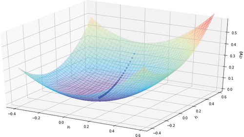
We set the parameter intercept ${\gamma }_0=0.0$ and the parameter slope ${\gamma }_1=0.5$. Therefore, we use the simulation to produce the balanced dataset of default and non-default events. For each of the true parameters and sample size of 6 400, the dataset was simulated and analyzed. To keep our model simple, we included only one predictor variable which is uniformly distributed (i.e., $X_i\sim U[-8;8])$ for which the cost function $\mathfrak{C}(\mathit{\gamma })$ is investigated. The dataset was simulated using the LRM and setting the parameter to 0.5 for a Bernoulli distribution resulting in a dichotomous response variable $Y_i$ indicating whether an event occurred or not.

Figure 1. Plot of a Cost Function$\mathfrak{C}(\mathit{\gamma })$for a simple binary LRM

The PD is then estimated through the use of LRM given in Equation (5)(5) $\mathfrak{C}(\mathit{\gamma })=-\frac{1}{n}\sum _{i=1}^n\left[Y_{i}ln({\pi }_i)+(1-Y_i)ln(1-{\pi }_i)\right].$(5) as

(30) $\mathfrak{P}{\mathfrak{D}}_i={\hat{\pi }}_i=\frac{1}{1+e^{(-{\hat{\gamma }}_0-{\hat{\gamma }}_1{X}_i)}}.$(30)

We use the accuracy rate $\mathfrak{A}$ to assess the performance of the optimized parameters in the model given in Equation (30)(30) $\mathfrak{P}{\mathfrak{D}}_i={\hat{\pi }}_i=\frac{1}{1+e^{(-{\hat{\gamma }}_0-{\hat{\gamma }}_1{X}_i)}}.$(30) , which is expressed as

(31) $\mathfrak{A}=\frac{{\sum }_{i=1}^n[I({\hat{\pi }}_i\ge 0.5)\equiv (Y_i=1)]+{\sum }_{i=1}^n[I({\hat{\pi }}_i<0.5)\equiv (Y_i=0)]}{n},$(31)

where $I(.)=\{0;1\}$ is the indicator function and $n$ is the sample size.

Figure 2. The plot of the cost function from five parameter estimators against number of iterations

Notes: The plots of the cost function values $\mathfrak{C}(\gamma )$ against the number of iterations $\mathfrak{I}$ per 100 iterations computed on the simulated dataset. The five parameter estimation methods are BGD, SGD, MBGD, IRLS and EM.

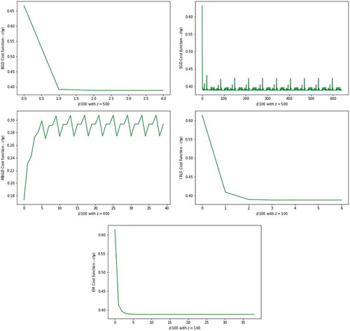
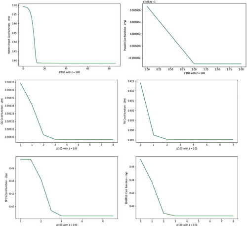
Figure 3. The plot of the cost function from six parameter estimators against number of iterations

Notes: The plots of the cost function values $\mathfrak{C}(\gamma )$ against the number of iterations $\mathfrak{I}$ per 100 iterations computed on the simulated dataset. The six parameter estimation methods are NM, PW, CG, TN, BFGS and LM-BFGS.

4. Applications to real dataset

This section is based on the application of the proposed methodology in section 2 to the benchmarking dataset. The anonymous dataset collected during the years 2016 to 2018 is from one of the South African financial institutions that provide loans to clients. The dataset contains the history of 1057 clients with the default indicator been the binary response variable ($Y$), i.e., default = 1 and non-default = 0. To empirically compare the simulation and the real data results, we only considered one predictor variable ($X_i$). This variable is the average percentage credit to disposable income of the clients recorded monthly over the given period.

Figure 4. The plot of the cost function from five parameter estimators against number of iterations for real dataset

Notes: The plots of the cost function values $\mathfrak{C}(\gamma )$ against the number of iterations $\mathfrak{I}$ per 100 iterations computed on the real given dataset. The five parameter estimation methods are BGD, SGD, MBGD, IRLS and EM.

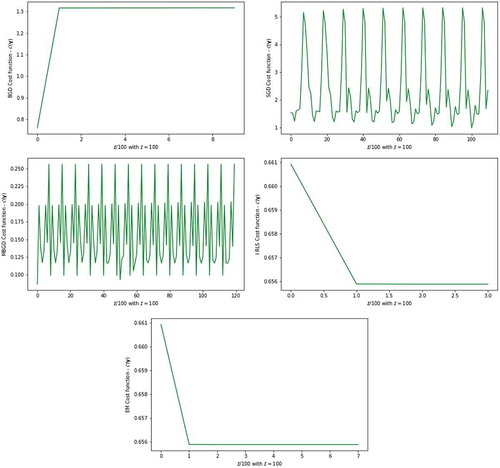
Figure 5. The plot of the cost function from six parameter estimators against a number of iterations for real dataset

Notes: The plots of the cost function values $\mathfrak{C}(\gamma )$ against the number of iterations $\mathfrak{I}$ per 100 iterations computed on the real given dataset. The six parameter estimation methods are NM, PW, CG, TN, BFGS and LM-BFGS.

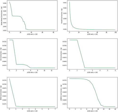
5. Results discussion

Tables 1 and 2 present the results of the optimized parameters for the binary LRM that minimizes the cost function, computed using 11 different parameter estimation methods. The corresponding graphical representations about the convergence of the parameter estimations cost function are presented in Figures 2–5.

Table 1. Parameter estimation method results for PD using Binary LRM

Parameter estimator	$\mathfrak{I}$	$\mathit{b}$	$\mathit{\kappa }(\epsilon )$	${\hat{\mathit{\gamma }}}_0$	${\hat{\mathit{\gamma }}}_1$	$\mathfrak{A}$	$\mathfrak{C}(\gamma )$
BGD	100	1	2(0.01)	0.0051	0.4914	0.8294	0.3881
SGD	100	1	10(0.01)	0.0075	0.4898	0.8294	0.3881
MBGD	100	1	10(0.01)	0.0099	0.4996	0.8292	0.2936
IRLS	100	1	7(1e-08)	0.0134	0.4930	0.8291	0.3881
EM	100	1	39 (1e-08)	0.0134	0.4930	0.8291	0.3881
NM	100	1	88 (1e-08)	0.0239	0.4977	0.8236	0.3853
PW	100	1	2 (1e-08)	0.0239	0.4977	0.8236	0.3853
CG	100	1	9 (1e-08)	0.0239	0.4977	0.8236	0.3853
TN	100	1	8 (1e-08)	0.0239	0.4977	0.8236	0.3853
BFGS	100	1	10 (1e-08)	0.0239	0.4977	0.8236	0.3853
LM-BFGS	100	1	9 (1e-08)	0.0239	0.4977	0.8236	0.3853

Notes: The results $\mathfrak{I}$ is the maximum number of iteration the method was set to, $b$ is the random mini-batch size, $\kappa$ is the number of iteration the method converged to and $\epsilon$ the tolerance level in brackets. For the gradient descent methods, the tolerance level is 0.01 and in all other methods it is smaller, i.e., 1e-08 = 0.00000008. ${\hat{\gamma }}_0$ and ${\hat{\gamma }}_1$ are, respectively, the intercept and slope estimated parameters. $\mathfrak{A}$ is the accuracy classification score given by Equation (31)(31) $\mathfrak{A}=\frac{{\sum }_{i=1}^n[I({\hat{\pi }}_i\ge 0.5)\equiv (Y_i=1)]+{\sum }_{i=1}^n[I({\hat{\pi }}_i<0.5)\equiv (Y_i=0)]}{n},$(31) . $\mathfrak{C}(\gamma )$ is the cost function for LRM defined in Equation (5)(5) $\mathfrak{C}(\mathit{\gamma })=-\frac{1}{n}\sum _{i=1}^n\left[Y_{i}ln({\pi }_i)+(1-Y_i)ln(1-{\pi }_i)\right].$(5) . NB for MBGD 40 sub-batches were generated from the sample size.

Table 2. Parameter estimation method results for PD using Binary LRM on real dataset

Parameter estimator	$\mathfrak{I}$	$\mathit{b}$	$\mathit{\kappa }(\epsilon )$	${\hat{\mathit{\gamma }}}_0$	${\hat{\mathit{\gamma }}}_1$	$\mathfrak{A}$	$\mathfrak{C}(\gamma )$
BGD	100	1	10(0.01)	0.1426	0.0883	0.6244	1.3172
SGD	100	1	10(0.01)	2.1909	0.1115	0.6244	2.3416
MBGD	100	1	10(0.01)	0.2211	0.1369	0.6244	0.2564
IRLS	100	1	4 (1e-08)	1.1281	−0.0179	0.6339	0.6559
EM	100	1	8 (1e-08)	1.1281	−0.0179	0.6339	0.6559
NM	100	1	85 (1e-08)	1.1281	−0.0179	0.6339	0.6559
PW	100	1	60 (1e-08)	1.1281	−0.0179	0.6339	0.6559
CG	100	1	14 (1e-08)	1.1281	−0.0179	0.6339	0.6559
TN	100	1	15 (1e-08)	1.1281	−0.0179	0.6339	0.6559
BFGS	100	1	8 (1e-08)	1.1281	−0.0179	0.6339	0.6559
LM-BFGS	100	1	17 (1e-08)	1.1281	−0.0178	0.6339	0.6559

Notes: For MBGD 12 sub-batches were generated from the sample size.

The BGD method described in Sub-Section 2.1 was configured to run 100 iterations for the simulated dataset but reveals the convergence of the cost function $\mathfrak{C}(\gamma )=0.3881$ in only two iterations (i.e. $\kappa =2$). For the real unbalanced dataset the method of BGD cost function value is very high. Figures 2 and 4 show the nature of convergence and its termination. The asymptotic rate of convergence can be inferior to alternative methods when there are many variables to work with. The method produced relatively reasonable cost function value with the learning rate of 0.01 while the parameter estimates are optimized, as illustrated by Figure 1. The SGD which is the simplified version of the BGD method has a premature convergence, as it is revealed in the real dataset shown in Figure 4 and the highest cost function of 2.3416. This is mainly due to the regular updates of the parameters through simulation (i.e., resampling without replacement for real dataset) and huge memory utilization for their storage, thus computationally expensive. Figure 2 for the SGD show that the method converges very fast but not with the exact optimum parameters, this is shown by the randomness of the cost function until all the configured iterations are executed.

IRLS and EM methods described in Sub-section 2.4 and Sub-section 2.5 reveals similar optimized parameters and minimized cost function values for the simulated and the real dataset. The only difference observed from the simulated dataset is on the convergence rate of the cost function, where IRLS method reaches convergence in only $\kappa =7$ iterations and terminate due to the tolerance $\epsilon =1e-08$, which is similar for the real dataset. EM method reaches convergence in 39 iterations and terminates with a tolerance $\epsilon =1e-08$. We observe that the tolerance criterion used for the EM method to be the size of the change in the cost function or parameter estimates from one iteration to the next. This is a measure for lack of progress but not of the actual convergence. We view this as a major drawback of the EM method. MBGD method computed with simulated dataset show optimum parameters very closed to the true parameters and the minimized cost function $\mathfrak{C}(\gamma )=0.2936$ among all the alternative optimization methods. MBGD method show to have reduced the variance of the parameter updates, which leads to more stable convergence of the cost function value between 0.25 and 0.31. Similarly, Figure 4—MBGD method for the real dataset the cost function obtained are between 0.1 and 0.25. According to Ruder (2016), MBGD does not always guarantee good convergence, but has few challenges that need to be taken into consideration when implemented. In this study MBGD shows very clear convergence and the challenge of the learning rate of 0.01 that we choose is efficient for the method. Also, the choice of the mini-batch size for the given sample size is important for the model. For the simulated dataset the mini-batch size is 40 and for the real dataset the mini-batch size is 12. The remainder of numerical optimization methods, i.e., NM, PW, CG, TN, BFGS and LM-BFGS, shows the same optimized parameters and cost functions with slightly different convergence information presented in Figures 3 and 5. The measure for lack of progress but not of the actual convergence is again observed for NM method. The progress in the convergence of the PW method is revealed to be fast, just like that of BGD for the simulated dataset. The progress in the convergence of the IRLS method is revealed to be fast for the given real dataset.

6. Conclusion

In Section 2, the binary LRM is proposed as a default model to assess model risk with respect to parameter estimation risk, that is an inappropriate parameter estimation method. The respective Sub-sections 2.1 to 2.11 describe recommended numerical optimization methods as parameter estimators for estimating the model parameters through minimization of the binary LRM cost function. It is revealed that parameter risk is important and essential through the comparison of numerical experiments and simulation done in section 3. MBGD method is shown to outperform the alternative optimization methods. MBGD estimators are accurate, since the bias is smaller among alternative methods, i.e.

$E({\hat{\gamma }}_1)-{\gamma }_1=0.4996-0.5=-0.0004$

Disregarding parameter risk can lead to a significant under-estimation of risk capital requirements, depending on the size of the underlying datasets. Therefore, we conclude that predicting PD using the binary LRM with the known varying thresholds will lead to substantially different results when parameter risk is taken into consideration. That is, when several optimization methods are employed. Numerical optimization estimation methods are identified as being the ones that have parameters which minimize the cost function or maximizes the log-likelihood function of the simple binary LRM. The impact of parameter estimation risk is depicted as an optimization method that yields the lowest cost function. Our experimental results support the need for further research of estimation parameter risk for binary LRM and other family of exponential models. Binary LRM with high order of predictor variables and interaction terms with different distributions may exhibit high parameter estimation risk implications. Therefore, it can be explored for further research on parameter estimation risk. Model risk management researchers and practitioners are therefore encouraged to consider parameter estimation risk through exploring different optimization methods as opposed to using the same traditional estimation methods repeatedly.

Additional information

Funding

This work was supported by the North-West University [P2A2B3] and BANKSETA.

Notes on contributors

Modisane B. Seitshiro

Modisane Seitshiro received his BSc degree in Statistics at North-West University (NWU), Mafikeng, South Africa (SA) in 2003. He completed MSc-Statistics in 2007 at NWU-Potchefstroom, SA. He was employed by Standard Bank SA, Corporate and Investment Banking in Market Risk for 6 years. He is currently employed by NWU-Vanderbijlpark as a Statistics Lecturer since 2013. He is a PhD student at the Unit for Business Mathematics and Informatics (BMI) at NWU. His research interests are Statistical Learning, Quantifying Model Risk and Margin Requirement.

Hopolang P. Mashele

Hopolang Mashele received his Mathematics PhD at the University of Witwatersrand, SA in 2001. He completed a Post-Doctoral Fellow at the Hungary Academy of Sciences in 2002. He was employed by Metropolitan Asset Management as an analyst in 2006. He is currently a Professor at the Centre for BMI at NWU. His research expertise are Approximation Theory, Derivatives Pricing and Financial Risk Management. Financial model risk is reduced by assessing different parameter estimators in this research and optimal estimator is retained.

References

- Agresti, A. (2015). Foundations of linear and generalized linear models. New Jersey: John Wiley and Sons.
- Agresti, A., & Kateri, M. (2011). Categorical data analysis. Heidelberg Berlin Germany: Springer.
- Albert, A., & Anderson, J. A. (1984). On the existence of maximum likelihood estimates in logistic regression models. Biometrika, 71(1), 1–20. doi:10.1093/biomet/71.1.1
- Alhawarat, A., Salleh, Z., Mamat, M., & Rivaie, M. (2017). An efficient modified Polak–Ribière–Polyak conjugate gradient method with global convergence properties. Optimization Methods and Software, 32(6), 1299–1312. doi:10.1080/10556788.2016.1266354
- Audet, C., & Tribes, C. (2018). Mesh-based Nelder–Mead algorithm for inequality constrained optimization. Computational Optimization and Applications, 71(2), 331–352. doi:10.1007/s10589-018-0016-0
- Babaie-Kafaki, S., & Ghanbari, R. (2015). A hybridization of the Polak-ribière-Polyak and Fletcher-Reeves conjugate gradient methods. Numerical Algorithms, 68(3), 481–495. doi:10.1007/s11075-014-9856-6
- Basel, I. (2004). International convergence of capital measurement and capital standards: A revised framework. Bank for international settlements.
- Borowicz, J. M., & Norman, J. P.(2006). The effects of parameter uncertainty in the extreme event frequency-severity model. 28th International Congress of Actuaries, Paris, (Vol. 28). France: Citeseer.
- Bottou, L. (2010). Large-scale machine learning with stochastic gradient descent. In Proceedings of COMPSTAT’2010 (pp. 177–186). France: Springer.
- Bottou, L. (2012). Stochastic gradient descent tricks. In Montavon G., Orr GB., and Muller KR (Eds.), Neural networks: Tricks of the trade (pp. 421–436). Heidelberg Berlin Germany: Springer.
- Candès, E. J., & SUR, P. (2018). The phase transition for the existence of the maximum likelihood estimate in high-dimensional logistic regression. arXiv Preprint arXiv:1804.09753.
- Caruana, J. (2010). Basel iii: Towards a safer financial system. Basel: BIS.
- Charalambous, C., Charitou, A., & Kaourou, F. (2000). Comparative analysis of artificial neural network models: Application in bankruptcy prediction. Annals of Operations Research, 99(1–4), 403–425. doi:10.1023/A:1019292321322
- Dembo, R. S., & Steihaug, T. (1983). Truncated-Newton algorithms for large-scale unconstrained optimization. Mathematical Programming, 26(2), 190–212. doi:10.1007/BF02592055
- Dempster, A. P., Laird, N. M., & Rubin, D. B. (1977). Maximum likelihood from incomplete data via the em algorithm. Journal of the Royal Statistical Society: Series B (Methodological), 39(1), 1–22.
- Derman, E. (1996). Model risk, quantitative strategies research notes. Goldman Sachs, New York, NY, 7, 1–11.
- Diers, D., Eling, M., & Linde, M. (2013). Modeling parameter risk in premium risk in multi-year internal models. The Journal of Risk Finance, 14(3), 234–250. doi:10.1108/JRF-11-2012-0084
- Dinse, G. E. (2011). An em algorithm for fitting a four-parameter logistic model to binary dose- response data. Journal of Agricultural, Biological, and Environmental Statistics, 16(2), 221–232. doi:10.1007/s13253-010-0045-3
- Hinton, G. E., Sabour, S., & Frosst, N. (2018). Matrix capsules with EM routing. International Conference on Learning Representations. Retrieved from https://openreview.net/forum?id=HJWLfGWRb
- Konečný, J., Liu, J., Richtárik, P., & Takàč, M. (2016). Mini-batch semi-stochastic gradient descent in the proximal setting. IEEE Journal of Selected Topics in Signal Processing, 10(2), 242–255. doi:10.1109/JSTSP.4200690
- Lagarias, J. C., Reeds, J. A., Wright, M. H., & Wright, P. E. (1998). Convergence properties of the Nelder–Mead simplex method in low dimensions. SIAM Journal on Optimization, 9(1), 112–147. doi:10.1137/S1052623496303470
- Laird, N., Lange, N., & Stram, D. (1987). Maximum likelihood computations with repeated measures: Application of the em algorithm. Journal of the American Statistical Association, 82(397), 97–105. doi:10.1080/01621459.1987.10478395
- Lindstrom, M. J., & Bates, D. M. (1988). Newton—Raphson and em algorithms for linear mixed-effects models for repeated-measures data. Journal of the American Statistical Association, 83(404), 1014–1022.
- Mashele, H. P. (2016). Aligning the economic capital of model risk with the strategic objectives of an enterprise (MBA Mini-dissertation), North-West University (South Africa), Potchefstroom Campus.
- Mclachlan, G., & Krishnan, T. (2007). The EM algorithm and extensions (Vol. 382). New Jersey, NJ: Wiley.
- Millar, R. B. (2011). Maximum likelihood estimation and inference: With examples in R, SAS and ADMB (Vol. 111). UK: Wiley.
- Minka, T. (2003). A comparison of numerical optimizers for logistic regression. Retrieved from https://tminka.github.io/papers/logreg/minka-logreg.pdf
- Nash, S. G., & Nocedal, J. (1991). A numerical study of the limited memory BFGS method and the truncated-Newton method for large scale optimization. SIAM Journal on Optimization, 1(3), 358–372. doi:10.1137/0801023
- Nelder, J. A., & Mead, R. (1965). A simplex method for function minimization. The Computer Journal, 7(4), 308–313. doi:10.1093/comjnl/7.4.308
- Neter, J., Kutner, M. H., Nachtsheim, C. J., & Wasserman, W. (1996). Applied linear statistical models (Vol. 4). New York, NY: Irwin Chicago.
- Nocedal, J., & Wright, S. (2006). Numerical optimization. New York, NY: Springer Science & Business Media.
- Noubiap, R. F., & Seidel, W. (2000). A minimax algorithm for constructing optimal symmetrical balanced designs for a logistic regression model. Journal of Statistical Planning and Inference, 91(1), 151–168. doi:10.1016/S0378-3758(00)00137-3
- Polyak, B. T., & Juditsky, A. B. (1992). Acceleration of stochastic approximation by averaging. SIAM Journal on Control and Optimization, 30(4), 838–855. doi:10.1137/0330046
- Powell, M. (1965). A method for minimizing a sum of squares of non-linear functions without calculating derivatives. The Computer Journal, 7(4), 303–307. doi:10.1093/comjnl/7.4.303
- Powell, M. J. (1964). An efficient method for finding the minimum of a function of several variables without calculating derivatives. The Computer Journal, 7(2), 155–162. doi:10.1093/comjnl/7.2.155
- Powell, M. J. (2007). A view of algorithms for optimization without derivatives. Mathematics Today-Bulletin of the Institute of Mathematics and Its Applications, 43(5), 170–174.
- Robles, V., Bielza, C., Larrañaga, P., González, S., & Ohno-Machado, L. (2008). Optimizing logistic regression coefficients for discrimination and calibration using estimation of distribution algorithms. Top, 16(2), 345. doi:10.1007/s11750-008-0054-3
- Ruder, S. (2016). An overview of gradient descent optimization algorithms. arXiv Preprint arXiv:1609.04747.
- Schiereck, D., Kiesel, F., & Kolaric, S. (2016). Brexit:(Not) another lehman moment for banks? Finance Research Letters, 19, 291–297. doi:10.1016/j.frl.2016.09.003
- Scott, J. G., & Sun, L. (2013). Expectation-maximization for logistic regression. arXiv Preprint arXiv:1306.0040.
- Shanno, D. F. (1970). Conditioning of Quasi-Newton methods for function minimization. Mathematics of Computation, 24(111), 647–656. doi:10.1090/S0025-5718-1970-0274029-X
- Shen, J., & He, X. (2015). Inference for subgroup analysis with a structured logistic-normal mixture model. Journal of the American Statistical Association, 110(509), 303–312. doi:10.1080/01621459.2014.894763
- Silvapulle, M. J. (1981). On the existence of maximum likelihood estimators for the binomial response models. Journal of the Royal Statistical Society. Series B (Methodological), 43(3), 310–313. doi:10.1111/rssb.1981.43.issue-3
- Tunaru, R. (2015). Model risk in financial markets: From financial engineering to risk management. Singapore: World Scientific.
- Vetterling, W. T., Teukolsky, S. A., Press, W. H., & Flannery, B. P. (1992). Numerical recipes: The art of scientific computing. (Vol. 2). Cambridge: Cambridge university press.
- Wang, H., Zhu, R., & Ma, P. (2018). Optimal subsampling for large sample logistic regression. Journal of the American Statistical Association, 113(522), 829–844. doi:10.1080/01621459.2017.1292914
- Yang, Y., Brown, T., Moran, B., Wang, X., Pan, Q., & Qin, Y. (2016). A comparison of iteratively reweighted least squares and Kalman filter with em in measurement error covariance estimation. 2016 19th International Conference on Information Fusion (FUSION) (pp. 286–291). Heidelberg Berlin Germany, IEEE.