Automatic time series modeling and forecasting: A replication case study of forecasting real GDP, the unemployment rate and the impact of leading economic indicators

Abstract

We test and report on time series modelling and forecasting using several US. Leading economic indicators (LEI) as an input to forecasting real US. GDP and the unemployment rate. These time series have been addressed before, but our results are more statistically significant using more recently developed time series modelling techniques and software. In this replication case study, we apply the Hendry and Doornik automatic time series PC-Give (AutoMetrics) methodology to the well-studied macroeconomic series, US. real GDP and the unemployment rate. The Autometrics system substantially reduces regression sum of squares measures relative to traditional variations on the random walk with drift model. The LEI are a statistically significant input to real GDP. A similar conclusion is found for the impact of the LEI and weekly unemployment claims series leading the unemployment rate series. We tested the forecasting ability of best univariate and best bivariate models over 60- and 120-period rolling windows and report considerable forecast error reductions. The adaptive averaging autoregressive model forecast ADA-AR and the adaptive learning forecast, ADL, produced the smallest root-mean-square errors and lowest mean absolute errors. Our results are greatly supportive of the significance for modeling and forecasting of the suggested input variables and they imply considerable improvements over all traditional benchmarks.

Keywords:

• adaptive learning forecasting automatic time series modelling
• forecasting
• leading indicators

JEL classifications:

• C32
• C50
• C51
• C53

1. Introduction

We test and report on time series modelling and forecasting using several US. Leading economic indicators (LEI) as an input to forecasting US. real GDP and the unemployment rate. These time series have been addressed before, but our results are more statistically significant using more recently developed time series modelling techniques and software. Montgomery, Zarnowitz, Tsay and Tiao (Montgomery et al., 1998) modelled the US. unemployment rate as a function of the weekly unemployment claims time series, 1948–1993. A similar conclusion is found for the impact of the LEI and weekly unemployment claims series leading the unemployment rate series. We employ the automatic time series modelling and forecasting of Hendry and Doornik (2014) and Doornik and Hendry (2015) where its emphasis on structural breaks is very relevant for modelling the MZTT unemployment rate data. We report statistically significant breaks in these data, 1959 to 1993 and 1959 to the present. The time series of the U.S. unemployment rate, the leading economic indicator and unemployment claims are shown in Figure 1. We tested univariate and best bivariate models over 60- and 120-period rolling windows and report highly significant forecast error reductions. The adaptive averaging autoregressive model ADA-AR and the adaptive learning forecast, ADL, produced the smallest root-mean-square errors and lowest mean absolute errors.

Figure 1. Time series plot of leading indicator, unemployment rate and unemployment claims

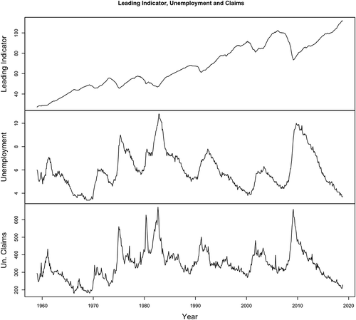
Figure 2. Coefficient estimates, 120-month rolling window, VAR(AIC) model, composite leading indicator

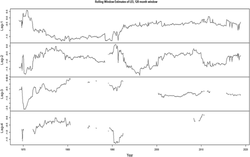
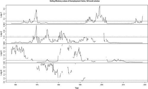
Figure 3. P-values of coefficient estimates, 120-month rolling window, VAR(AIC) model, LEI

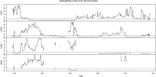
Figure 4. Coefficient estimates, 120-month rolling window, VAR(AIC) model, weekly unemployment claims

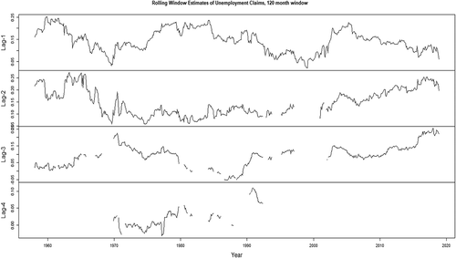
Figure 5. P-values of coefficient estimates, 120-month rolling window, VAR(AIC) model, weekly unemployment claims.

As an introductory example, let us consider the US. real GDP as can be represented by an autoregressive integrated moving average (ARIMA) model. The data are differenced to create a process that has a (finite) mean and variance that do not change over time and the covariance between data points of two series depends upon the distance between the data points, not on the time itself—a transformation to stationarity. Thus, it is assumed that the raw data, with or without a logarithmic transformation, form an integrated (non-stationary) process, and the characteristics of such a process can be concisely be modelled as follows:

(1) $\phi \left(\mathrm{B}\right){\left(1-B\right)}^d{X}_t=\theta \left(\mathrm{B}\right){\epsilon }_t$(1)

where ϕ(B) and θ(B) are the autoregressive and moving average polynomials in the backward operator B, of orders p and q, ε_t is a white noise error term and d is an integer representing the order of the data differencing. In economic time series, a first-difference of the data is normally performed.¹ The application of the differencing operator, d, produces a stationary autoregressive moving average ARMA(p, q) model when all parameters are constant across time. Many economic series can be modelled with a simple subset of the class of ARIMA(p, d, q) models, particularly the random walk with drift and a moving average term such as below:

(2) $\mathrm{\Delta }{X}_t=\mu +{\epsilon }_t+\theta {\epsilon }_{t-1}.$(2)

This model of economic time series behaviour is not new and can be traced back to the works of Box and Jenkins (1970), Granger and Newbold (1977), and Nelson and Plossner (1982).

One can find, examine and download the real Gross Domestic Product from the St. Louis Federal Reserve bank database, FRED, as we do, or The Conference Board Business Cycle database. The data are downloaded from the first quarter of 1959 to the second quarter of 2018. An ARIMA(1, 1, 0) model is cursory estimated as an illustration and the results provided are²

(3) $\mathrm{\Delta }{X}_t={0.0053}_{\left(7.62\right)}+{0.2922}_{\left(4.62\right)}\mathrm{\Delta }{X}_{t-1}$(3)

where the parentheses indicate the corresponding (absolute values of the) t-statistics of the estimated parameters. This model’s fit, measured by its residual sum of squares (RSS), is 0.0145.

Our analysis is composed of six sections. The first section is the introduction to our replication study of the US. unemployment rate. The second section is a brief discussion of David Hendry and his colleagues’ research into automatic time series model selection. The third section presents evidence regarding automatic time series modelling of US. real GDP using the leading economic indicators, LEI, time series. The fourth section presents evidence regarding automatic time series modelling the US. unemployment rate with the LEI time series. The fifth section of our analysis presents adaptive learning forecasting results of the US. unemployment rate as a function of LEI.

The sixth section is the conclusion. We report that the US. LEI time series continues to be statistically significant in forecasting US. real GDP. We report that the weekly unemployment claims time series studied in the seminal Montgomery et al. (1998) study continues to be highly statistically significant in modelling the US. unemployment rate. Moreover, we report that newer methodologies, the Autometrics time series software and adaptive learning forecasting offer additional statistical association regarding the relationship among LEI, the monthly unemployment claims and the unemployment rate. We replicate the seminal study and extend the analysis to 2018. LEI and one of its components, the unemployment claims time series, lead the unemployment rate.

2. Automatic time series model selection

Automatic time series models have recently been discussed in Hendry (1986), Krolzig and Hendry (2001), and Hendry & Krolzig (2005), Hendry and Nielsen (2007), Castle et al. (2013), and Hendry and Doornik (2014) and implemented in the Autometrics software.³ Hendry sets the tone for automatic modelling by contrasting how statistically—based his PC-Give and Autometrics work in contrast to the “data mining” and “garbage in, garbage out” routines, citing their forecasting efficiency and performance. If one starts with a large number of predictors, or candidate explanatory variables, say n, then the general model can be written:

(4) $y_t={\sum }_{i=1}^n{\gamma }_i{Z}_{it}+u_t$(4)

The (conditional) data generating processes are assumed to be given by

(5) $y_t={\sum }_{i=1}^n{\beta }_i{Z}_{\left(i\right),t}+{ϵ}_t$(5)

where ${ϵ}_t\cong IN\left(0,{\sigma }_e^2\right)$ for any n ≤ N.

One must select the relevant regressors where ${\beta }_j\ne 0$in (5). Hendry and his colleagues refer to Equation (4)(4) $y_t={\sum }_{i=1}^n{\gamma }_i{Z}_{it}+u_t$(4) as the most general, statistical model that can be postulated, given the availability of data and previous empirical and theoretical research as the general unrestricted model (GUM). The Hendry general-to-specific modelling process is referred to as Gets. One seeks to identify all relevant variables, the relevant lag structure and cointegrating relations, forming near orthogonal variables, Z. The general unrestricted model, GUM, with s lags of all variables can then be written:

(6) $y_t={\sum }_{i=1}^n{\sum }_{j=0}^s{\beta }_{i,j}{x}_{i,t-j}+{\sum }_{i=1}^n{\sum }_{j=0}^s{k}_{i,j}{z}_{i,t-j}+{\sum }_{j=1}^s{\theta }_j{y}_{t-j}+{\sum }_{i=1}^T{\delta }_i{1}_{\left\{i=t\right\}}+e_t,$(6)

where${\epsilon }_t\text{~}\mathrm{I}\mathrm{N}\left(0,{\sigma }_e^2\right)$. Furthermore, outliers and shifts for T observations can be modelled with saturation variables, see Doornik and Hendry (2015) and Hendry and Doornik (2014, Chapters 7, 14).

Automatic modelling seeks to eliminate irrelevant variables; variables with insignificant estimated coefficients; lag-length reductions; and reducing saturation variables (for each observation); the nonlinearity of the principal components; and combinations of “small effects” represented by principal components.⁴ One can consider the orthogonal regressor case in which one ranks the variables by their t-statistics, highest to lowest and defines m to be the smallest, but statistically significant t-statistic, $t_m^2$, and discards all variables with t-statistics below the m largest t-values. One must be reminded that every test statistic has a distribution occurring in different samples by the specification of Equations (5)(5) $y_t={\sum }_{i=1}^n{\beta }_i{Z}_{\left(i\right),t}+{ϵ}_t$(5) and (6(6) $y_t={\sum }_{i=1}^n{\sum }_{j=0}^s{\beta }_{i,j}{x}_{i,t-j}+{\sum }_{i=1}^n{\sum }_{j=0}^s{k}_{i,j}{z}_{i,t-j}+{\sum }_{j=1}^s{\theta }_j{y}_{t-j}+{\sum }_{i=1}^T{\delta }_i{1}_{\left\{i=t\right\}}+e_t,$(6) ). We seek to select a model of the form:

(7) $y_t={\sum }_{r=1}^m{\delta }_r{Z}_{\left\{r\right\},t}+n_t$(7)

where $Z_{\left\{r\right\},t}$ is a subset of the initial N variables, and that model may differ from either the one postulated in (4), (5), (6) or (7) depending on which variables remain at the end of the selection process.⁵ One progresses from the general unrestricted model to the “final” model in (7) by establishing that model residuals are approximately normal, homoscedastic and independent. Model reduction proceeds by tree searches of insignificant variables. The last, non-rejected model is referred to as the terminal equation. Selected model regressors have coefficients that are large relative to their estimated standard errors; since the estimators obtained by the initial model (5) are unbiased, the selected estimators are upward-biased conditional on retaining $Z_{\left(j\right),t}$. The unselected variables will have downward-biased estimators. By omitting irrelevant variables, the selection model does not “overfit” the model and the relevant (retained) variables have estimated standard errors close to those from fitting Equation (7)(7) $y_t={\sum }_{r=1}^m{\delta }_r{Z}_{\left\{r\right\},t}+n_t$(7) .

The automatic time series modelling program (PCGets) or (Autometrics) is efficient, but Hendry and Nielsen (2007) state that the largest selection bias can arise from strongly correlated regressors. Autometrics deals with outliers and breaks in its automatic time series modelling. The regression sum of squares, RSS, rises as the outlier criteria shrink. Autometrics apply can indicator-indicator saturation (IIS) variables, step-indicator saturation (SIS) variables, differenced IIS (DIIS) and trend saturation (TIS) to all marginal models where there are significant indicators. The step-indicator saturation (SIS) variables are generalized IIS variables with higher statistical power to detect location shifts. One can include outlier detection indicators (impulse-indicator saturation, I, and step-indicator saturation, S) in the Autometrics analysis of the LEI component effectiveness estimates.⁶ For now, we present in the table the application of the automatic time series modelling procedure of the OxMetrics system to estimate a more adequate model for real GDP, the expansion of the model in (3) but with the inclusion of time indicator variables; the raw results of the program are presented below:

(8) $\mathrm{\Delta }{X}_t={0.0052}_{\left(8.15\right)}+{0.3012}_{\left(5.23\right)}\mathrm{\Delta }{X}_{t-1}+{0.0249}_{\left(3.48\right)}{I}_{t:44}+{0.0317}_{\left(4.49\right)}{I}_{t:77}-{0.0269}_{\left(3.81\right)}{I}_{t:85}-{0.0254}_{\left(3.58\right)}{I}_{t:199},$(8)

where the indicator variables indicate the sample point shift (e.g., t:44 indicates a break at sample point 44) and the RSS now drops to 0.0115 compared to 0.0145 of the ARIMA(1, 1, 0) model.⁷ It is important to note that in this model neither the initial estimates of the drift and autoregressive term change (compared to Equation (3)(3) $\mathrm{\Delta }{X}_t={0.0053}_{\left(7.62\right)}+{0.2922}_{\left(4.62\right)}\mathrm{\Delta }{X}_{t-1}$(3) ) and all terms are automatically significant.

Hendry and his colleagues stress a major source of non-stationarity is due to structural breaks; changes in the parameters generating the data, see Hendry and Nielsen (2007) and Castle et al. (2013), among many others. They argue that location shifts, shifts in the coefficients of deterministic terms such as long-run means, trends and growth rates can generate such non-stationarity.

We will now illustrate this using the raw, not differenced, data on real GDP and Autometrics. In Table 1 that follows (we use a table to illustrate the results so that the reader can view the relevant statistics) we present the initial results for the simple AR(1) model for real GDP and another one from the application of Autometrics (model I) using many indicator variables that capture such structural breaks. Note the implications for residual diagnostics, as the inclusion of the indicator functions makes the model congruent and consistent with the assumptions behind the general-to-specific approach. The results are highly illustrative. First, as expected, a simple AR(1) model simply produces the well-known result that first differencing of the series is suggested and that anything else that remains after differencing must be modelled separately.

Table 1. Autometrics analysis of levels of real GDP data

	Plain AR(1) model	Autometrics model I	Autometrics model II
Lagged real GDP	1.004 (significant at 1%)	0.619 (significant at 1%)	1.006 (significant at 1%)
Lagged real GDP partial R^2	99.9%	56.8%	99.9%
Number of indicators	0	30 (all significant at 1%)	28 (9 significant at 5%, 10 significant at 10%
RSS	591.309	168.732	195.091
AR 1–2 test (p-value)	0.00	0.17	0.64
Normality test (p-value)	0.00	0.23	0.01
Heteroscedasticity test (p-value)	0.00	0.14	0.32

There is a clear presence of autocorrelation, heteroscedasticity and non-normality in the residuals. However, passing the series to Autometrics and using indicator functions we find, not only a major reduction in the residual sum of squares but other interesting results: first, the relative contribution of the lagged real GDP drops from 99.9% on the simple AR(1) model to a reasonable 56.8% in the Autometrics model and, moreover, note the serious reduction in the estimates magnitude: once structural breaks have been accounted for the memory of the series drops from a value of unity (unit root non-stationarity) to a value of 0.62 well within the confines of autoregressive stationarity—thus the non-stationary components are essentially the shifts that are being captured by the indicator functions (all of which are highly significant). It is also interesting to note that there are at least two indicator functions that have a partial R² above 25%, meaning that they do capture a significant part of the variability of the series. Finally, it is evident that modelling the structural breaks removed the autocorrelation, heteroscedasticity and non-stationarity as can be seen by the increased p-values of all relevant tests in the table.

The perceptive reader will ask whether there is a unique model that can be used to capture the salient features of the levels data via an automated procedure; the answer would be yes if all possible indicators are included—but often times this will be difficult due to degrees of freedom constraints. Thus, we illustrate the change in results if we use more initial indicators than in Table 1, namely all possible IIS, SIS, DIIS and TIS variables. The reader is referred to Doornik (2009), Doornik and Hendry (2013, 2015) for the AutoMetrics estimation procedures and saturation variable modeling with Ox Metrics. The results are summarized in the second Autometrics model of Table 1, model II. It is clear that this second model provides reductions in the p-values for autocorrelation and heteroscedasticity at the cost of non-normality in the residuals and a higher RSS value. The reader could have used robust regression, as shown in Dhrymes (2017) and  Maronna et al., (2019) to estimate traditional regression models. Furthermore, we can see that the estimate of the lagged value of real GDP is essentially unity, which suggests a difference-based model should be used here. The extend on which such trade-off on the p-values is useful it is debatable and the results indicate that some a priori considerations should be given to the type of indicators one uses.

3. Automatic time series modelling of real GDP using leading economic indicators (LEI)

The composite indexes of leading (LEI), coincident and lagging indicators produced by The Conference Board are summary statistics for the US. economy. Wesley Clair Mitchell of Columbia University constructed the indicators in 1913 to serve as a barometer of economic activity. The leading indicator series was developed to turn upward before aggregate economic activity increased, and decrease before aggregate economic activity diminished. Historically, the cyclical turning points in the leading index have occurred before those in aggregate economic activity, cyclical turning points in the coincident index have occurred at about the same time as those in aggregate economic activity, and cyclical turning points in the lagging index generally have occurred after those in aggregate economic activity.

The Conference Board’s components of the composite leading index for the year 2002 reflected the work and variables shown in Zarnowitz (1992) list, which continued work of the Mitchell (1913), Burns and Mitchell (1946), and Moore (1961).⁸ The Conference Board composite index of leading economic indicators, LEI, is an equally weighted index in which its components are standardized to produce constant variances.⁹ Let us now examine the effectiveness of changes in the LEI to be statistically associated with future changes (growth) in real GDP over the 1959-2018Q1 period. The present (September 2016) 10 components of The Conference Board Leading Economic Index® for the US. include

1. Average weekly hours, manufacturing

2. Average weekly initial claims for unemployment insurance

3. Manufacturers’ new orders, consumer goods and materials

4. ISM® Index of New Orders

5. Manufacturers’ new orders, nondefense capital goods excluding aircraft orders

6. Building permits, new private housing units

7. Stock prices, 500 common stocks

8. Leading Credit Index™

9. Interest rate spread, 10-year Treasury bonds less federal funds

10. Average consumer expectations for business conditions.

A database of the monthly leading economic indicators is merged with the quarterly FRED database for the real GDP growth previously analyzed. We test the hypothesis that the changes LEI lead real GDP growth. One can examine whether real GDP growth is statistically associated with contemporaneous and one through four-quarter lags in the LEI, denoted by L_t below.¹⁰ The results on Equation (9)(9) $\mathrm{\Delta }{X}_t=-{0.0002}_{\left(0.07\right)}+{0.2792}_{\left(4.40\right)}\mathrm{\Delta }{X}_{t-1}-{10.473}_{\left(0.55\right)}\mathrm{\Delta }{L}_{t-1}+{5.359}_{\left(0.27\right)}\mathrm{\Delta }{L}_{t-2}-{19.64}_{\left(1.00\right)}\mathrm{\Delta }{L}_{t-3}-{8.885}_{\left(0.47\right)}\mathrm{\Delta }{L}_{t-4}$(9) show that none of the four lags is significant while the estimation of the first lag of the real GDP growth remains robust:

(9) $\mathrm{\Delta }{X}_t=-{0.0002}_{\left(0.07\right)}+{0.2792}_{\left(4.40\right)}\mathrm{\Delta }{X}_{t-1}-{10.473}_{\left(0.55\right)}\mathrm{\Delta }{L}_{t-1}+{5.359}_{\left(0.27\right)}\mathrm{\Delta }{L}_{t-2}-{19.64}_{\left(1.00\right)}\mathrm{\Delta }{L}_{t-3}-{8.885}_{\left(0.47\right)}\mathrm{\Delta }{L}_{t-4}$(9)

and there is a rise in the RSS compared to the model with indicator variables but (naturally) a decrease in the RSS compared to the ARIMA(1, 1, 0) model, at 0.0136. However, once outliers are allowed to enter and accounted for in the model via the automatic modelling approach we find that the 3-period lag of the leading economic indicator becomes strongly significant as follows:

(10) $\mathrm{\Delta }{X}_t={0.1647}_{\left(3.16\right)}\mathrm{\Delta }{X}_{t-1}+{6.7523}_{\left(5.23\right)}\mathrm{\Delta }{L}_{t-3}+I_t$(10)

and we can see that the estimate of the first lag of the real GDP is reduced to about half and the third lag of the leading indicator becomes highly significant; we omit the many indicator terms that we put collectively at the vector I_t; all estimates are as expected highly significant and the RSS now drops to 0.0075 (again, a rather natural result because of the presence of more indicator variables—but what is important to understand now is that the RSS decrease is obtained by a coherent and congruent statistical approach).¹¹ Automatic time series modelling using Autometrics of the OxMetrics system via sequential least squares regression analysis is useful in reducing the residual sum of squares and improving the fit of the models considered. Although of limited presence in the above equation, The Conference Board LEI and its components are potential barometers of future economic growth, based on their potential on modelling and forecasting—which we also discuss at the forecasting section of the paper.

We repeat the analysis of Table 1 for the levels of real GDP while now including four lags of the leading indicator variable and, then, we repeat the Autometrics exercise that we performed before with the inclusion of additional indicators. The results are given in Table 2 and are again very illuminating and similar to Table 1, with two major differences. First, observe that the reduction in RSS in very small by the inclusion of the lagged LEI (which is significant nevertheless) and that lagged LEI contribute an additional relative 3.31% in explaining the variability of the level of real GDP; furthermore, note that the presence of the LEI removes heteroscedasticity. Second, when we turn to the Autometrics, the LEI is no longer a remaining variable and although the results are as before (as in Table 1); note that we have 27 instead of 30 indicator functions and the order of elimination now removed some indicators and created heteroscedasticity. Some discretion, therefore, is indeed advised and we could possibly envision re-introducing the LEI in the final Autometrics model. This goes, however, beyond our scope and we do not discuss it any further. However, as we did with the comparison of Autometrics models in Table 1 we again consider additional indicators in another attempt to model the levels of the real GDP with the LEI present and, furthermore, to reduce the clear presence of heteroscedasticity that appears in Autometrics model I of Table 2.

Table 2. Autometrics analysis of levels real GDP data, LEI included

	AR(1) Model + leading indicator lags	Autometrics model I	Autometrics model II
Lagged real GDP, lag 1	0.9942 (significant at 1%)	0.7010 (significant at 1%)	1.3574 (significant at 1%)
Lagged real GDP, lag 1, partial R^2	99.7%	67.2%	77.2%
Lagged real GDP, lag 2	n.a.	n.a.	−0.3615 (significant at 1%)
Lagged real GDP, lag 2, partial R^2	n.a.	n.a.	19.7%
Contemporaneous LEI	n.a.	n.a.	1.3572 (significant at 5%)
Contemporaneous LEI partial R^2	n.a.	n.a.	3.51%
Lagged LEI, lag 1	2.1675 (significant at 1%)	n.a.	n.a.
Lagged LEI partial R^2	3.31%	n.a.	n.a.
Number of indicators	0	27 (all significant at 1%)	21 (7 significant at 5%, 8 significant at 10%)
RSS	552.914	184.280	237.785
AR 1–2 test (p-value)	0.00	0.36	0.07
Normality test (p-value)	0.00	0.24	0.08
Heteroscedasticity test (p-value)	0.16	0.01	0.47

The same kind of qualitative results as in Table 1 appears in model II of Autometrics in Table 3. That is, we find again a trade-off in terms of the statistics for heteroscedasticity and the rest of the results vis-à-vis Autometrics model I. There is higher persistence for the two lags of real GDP in model II, less significant indicator, higher RSS compared to model I but also a marked absence of heteroscedasticity. If we combine the results of Tables 1 and 2 we can actually draw a practical conclusion: it appears that, for the levels of real GDP, the source of heteroscedasticity is on the presence of particular kinds of breaks that are captured by the indicators of model II—this, however, comes at a cost to other statistics such as the RSS and the increased p-values on autocorrelation and normality. The final model choice probably should be made on some additional considerations or a different search procedure might be tried otherwise.

4. Automatic time series modelling of the unemployment rate using leading economic indicators (LEI)

Another widely studied time series is the (US) unemployment rate. Montgomery, Zarnowitz, Tsay and Tiao (Montgomery et al., 1998) modelled the quarterly unemployment rate for the 1948 to 1993 period and reached several very interesting conclusions. Among the conclusions, the unemployment rate contained no consistent trend, and in times of rising unemployment, the weekly unemployment insurance claims, UIC, were a useful input—however unemployment claims were not useful over the entire 1948–1993 time period. MZTT suggested that although future models could build upon asymmetric modelling analysis, long-run models had to forecast stable, slowing declining periods of unemployment. To set up the stage for our later discussion we first consider an ordinary least squares regression model for the 1959–1993 time period, i.e., the original period of the MZTT analysis, with changes in unemployment, denoted as ΔΧ_t, and the differenced log-weekly unemployment claims data, denoted as ΔL_t, with nine lags of unemployment claims, one reports results that are clearly consistent with the explanatory power of unemployment claims for the change in unemployment. Our results appear in Equation (11)(11) $\mathrm{\Delta }{X}_t=-{0.2035}_{\left(3.93\right)}\mathrm{\Delta }{X}_{t-1}+{1.0578}_{\left(6.64\right)}\mathrm{\Delta }{L}_{t-1}+{0.9123}_{\left(5.87\right)}\mathrm{\Delta }{L}_{t-2}+{0.6485}_{\left(4.19\right)}\mathrm{\Delta }{L}_{t-3}+{0.4676}_{\left(3.08\right)}\mathrm{\Delta }{L}_{t-4}+{0.5806}_{\left(3.83\right)}\mathrm{\Delta }{L}_{t-5}+{0.3427}_{\left(2.25\right)}\mathrm{\Delta }{L}_{t-6}+{0.5687}_{\left(3.76\right)}\mathrm{\Delta }{L}_{t-7}+{0.1514}_{\left(0.99\right)}\mathrm{\Delta }{L}_{t-8}+{0.6129}_{\left(4.08\right)}\mathrm{\Delta }{L}_{t-9}$(11) :

(11) $\mathrm{\Delta }{X}_t=-{0.2035}_{\left(3.93\right)}\mathrm{\Delta }{X}_{t-1}+{1.0578}_{\left(6.64\right)}\mathrm{\Delta }{L}_{t-1}+{0.9123}_{\left(5.87\right)}\mathrm{\Delta }{L}_{t-2}+{0.6485}_{\left(4.19\right)}\mathrm{\Delta }{L}_{t-3}+{0.4676}_{\left(3.08\right)}\mathrm{\Delta }{L}_{t-4}+{0.5806}_{\left(3.83\right)}\mathrm{\Delta }{L}_{t-5}+{0.3427}_{\left(2.25\right)}\mathrm{\Delta }{L}_{t-6}+{0.5687}_{\left(3.76\right)}\mathrm{\Delta }{L}_{t-7}+{0.1514}_{\left(0.99\right)}\mathrm{\Delta }{L}_{t-8}+{0.6129}_{\left(4.08\right)}\mathrm{\Delta }{L}_{t-9}$(11)

where the fit of the model is with an RSS of 11.17 and with an R-squared of 26.3%. All explanatory variables are highly significant, save the eighth lag. A similar set of results is produced if we consider a robust regression estimation approach, and they are available upon request. The estimation results of Equation (11)(11) $\mathrm{\Delta }{X}_t=-{0.2035}_{\left(3.93\right)}\mathrm{\Delta }{X}_{t-1}+{1.0578}_{\left(6.64\right)}\mathrm{\Delta }{L}_{t-1}+{0.9123}_{\left(5.87\right)}\mathrm{\Delta }{L}_{t-2}+{0.6485}_{\left(4.19\right)}\mathrm{\Delta }{L}_{t-3}+{0.4676}_{\left(3.08\right)}\mathrm{\Delta }{L}_{t-4}+{0.5806}_{\left(3.83\right)}\mathrm{\Delta }{L}_{t-5}+{0.3427}_{\left(2.25\right)}\mathrm{\Delta }{L}_{t-6}+{0.5687}_{\left(3.76\right)}\mathrm{\Delta }{L}_{t-7}+{0.1514}_{\left(0.99\right)}\mathrm{\Delta }{L}_{t-8}+{0.6129}_{\left(4.08\right)}\mathrm{\Delta }{L}_{t-9}$(11) are supporting the MZTT argument on the usefulness of the unemployment claims and, in general, are supporting the notion that the explanatory variable can act as a possible predictor of the changes in unemployment.

We next take another look at the MZTT data and update the analysis for the 1959–October 2018, using The Conference Board LEI data, which contains weekly unemployment claims as a component to its leading economic indicators. As above, we difference the unemployment rate, the leading economic indicator and the and weekly unemployment insurance claims for the analysis; in the equations below we keep the same notation as in Equation (11)(11) $\mathrm{\Delta }{X}_t=-{0.2035}_{\left(3.93\right)}\mathrm{\Delta }{X}_{t-1}+{1.0578}_{\left(6.64\right)}\mathrm{\Delta }{L}_{t-1}+{0.9123}_{\left(5.87\right)}\mathrm{\Delta }{L}_{t-2}+{0.6485}_{\left(4.19\right)}\mathrm{\Delta }{L}_{t-3}+{0.4676}_{\left(3.08\right)}\mathrm{\Delta }{L}_{t-4}+{0.5806}_{\left(3.83\right)}\mathrm{\Delta }{L}_{t-5}+{0.3427}_{\left(2.25\right)}\mathrm{\Delta }{L}_{t-6}+{0.5687}_{\left(3.76\right)}\mathrm{\Delta }{L}_{t-7}+{0.1514}_{\left(0.99\right)}\mathrm{\Delta }{L}_{t-8}+{0.6129}_{\left(4.08\right)}\mathrm{\Delta }{L}_{t-9}$(11) . We first estimate an ARIMA(1,1,0) model for the unemployment rate for 1959–1994, the same model we estimated for the real GDP growth and the results are below:

(12) $\mathrm{\Delta }{X}_t=-{0.0017}_{\left(0.21\right)}+{0.0807}_{\left(1.79\right)}\mathrm{\Delta }{X}_{t-1}$(12)

where the fit of the model is indicated by an RSS of 15.98. We then proceed to use the automatic time series approach and include explanatory variables and indicator functions. As before we report the variables that have economic interpretation on the right-hand side:

(13) $\mathrm{\Delta }{X}_t=-{0.2654}_{\left(6.40\right)}\mathrm{\Delta }{X}_{t-1}+{0.002}_{\left(5.52\right)}\mathrm{\Delta }{L}_{t-1}+{0.002}_{\left(5.66\right)}\mathrm{\Delta }{L}_{t-2}\mp {0.0016}_{\left(4.54\right)}\mathrm{\Delta }{L}_{t-3}+{0.001}_{\left(3.15\right)}\mathrm{\Delta }{L}_{t-4}+{0.0013}_{\left(4.09\right)}\mathrm{\Delta }{L}_{t-6}+{0.0012}_{\left(4.09\right)}\mathrm{\Delta }{L}_{t-9}+I_t$(13)

where all the estimates are highly significant and the RSS drops to 9.12, as again expected, and where we can make two interesting observations: first, note that the autoregressive parameter turns negative and about of the same magnitude as the autoregressive parameter on the real GDP equation; second, the estimates of the lags of the weekly unemployment claims (now taking the place of the leading indicator) are almost all of the same size and always positive—the interpretation is straightforward and economically plausible: a rise in any of the past quarters in the unemployment claims leads to an expected rise in unemployment in the future and the total (cumulative) effect of unemployment claims is about 0.009 as the sum of the estimated coefficients. The negative sign of the autoregressive parameter indicates the stronger cyclical characteristics of the unemployment series, compared to those of the real GDP growth. Switching now to the post-1994 period, and re-estimating the above two equations for the 1994–2018 time period and find that, post-publication, the relationship is still maintained as follows, first for the ARIMA(1,1,0) model:

(14) $\mathrm{\Delta }{X}_t=-{0.0088}_{\left(0.55\right)}-{0.1275}_{\left(1.37\right)}\mathrm{\Delta }{X}_{t-1}$(14)

where we can see that the autoregressive parameter becomes negative and less significant (the RSS here being 3.40 so the fit here is much better). The corresponding results from the use of the automatic procedure using the weekly unemployment claims are given below:

(15) $\mathrm{\Delta }{X}_t=-{0.3603}_{\left(4.18\right)}\mathrm{\Delta }{X}_{t-1}+{0.0025}_{\left(2.67\right)}\mathrm{\Delta }{L}_{t-2}+{0.005}_{\left(5.18\right)}\mathrm{\Delta }{L}_{t-3}+{0.0021}_{\left(2.08\right)}\mathrm{\Delta }{L}_{t-4}+{0.003}_{\left(3.00\right)}\mathrm{\Delta }{L}_{t-5}+{0.0031}_{\left(3.18\right)}\mathrm{\Delta }{L}_{t-6}+{0.0029}_{\left(3.07\right)}\mathrm{\Delta }-{0.0021}_{\left(2.65\right)}\mathrm{\Delta }{L}_{t-10}+I_t,$(15)

where now the total impact from the leading indicator variable is higher to 0.0165 and the autoregressive parameter remains again significant and negative—the RSS is now even lower at 1.99.

A similar set of results, statistically and conceptually, is obtained when we substitute the weekly unemployment claims with the composite leading indicator, still being in the post-MZTT publication period, of after 1994 to 2018, and are as follows:

(16) $\mathrm{\Delta }{X}_t={0.0045}_{\left(2.59\right)}-{0.2259}_{\left(2.90\right)}\mathrm{\Delta }{X}_{t-1}-{0.1813}_{\left(2.65\right)}\mathrm{\Delta }{L}_{t-2}-{0.1892}_{\left(2.58\right)}\mathrm{\Delta }{L}_{t-3}+I_t,$(16)

and the fit of the model is with an RSS of 2.03 (almost identical with that of the model above with the unemployment claims), with the estimates in front of the leading indicator being now (as expected) negative and again of about the same size—the differences in magnitude with the weekly unemployment claims are in the units of measurement, the unemployment claims being measured in a real-life measure of thousands of unemployed (check). Finally, we re-estimate the two equations of the weekly unemployment claims and the composite leading indicator for the whole sample period from 1959 to 2018 and the results obtained verify the previous ones, as to that both variables lead unemployment.

As in the case of the real GDP series, we next use Autometrics on the raw, not differenced, data, on the unemployment rate series. We collect our results on Tables 3a and 3b, in a similar fashion to Tables 1 and 2. Here we prepare two tables due to the number of models that we will have to consider: the first group of models is in Table 3a and the second group of models is in Table 3b. Starting off with Table 3a we have four models, the plain AR(1) model, an AR(1) model with indicator functions only, and then the AR(1) model with indicators plus the weekly claims and the LEI components (separately). We report the search results of Autometrics in the table and we can see immediately some very interesting results. First, note that a simple autoregression does not capture the cyclical variability of the level of unemployment as expected, with a low estimate of persistence and a relatively low R². The RSS is large, and there are autocorrelation, heteroscedasticity and non-normality in the residuals. Adding indicators in this first model we find, as before in the case of the real GDP series, that the RSS is greatly reduced, autocorrelation disappears as does heteroskedasticity, but not non-normality—note that we have a total of 47 significant indicators. Adding to this last model, the weekly claims we can obtain even further RSS reduction, at the expense of about 20 more indicators but the weekly claims add explanatory power (although at about the 10% partial R²); thus, Autometrics does capture the empirical finding of weekly claims being a reasonable explanatory variable for the unemployment rate. Note that the normality test indicates now some improvement although we have a deterioration to the p-values of autocorrelation and heteroscedasticity (that nevertheless remain into the close to 5% to 10% territory).

Finally, the fourth model we examine contains the LEI lags in addition to the variables of the second model, but not the unemployment claims. The number of indicator variables increases to 65, all significant, and we can clearly see that the lags of the LEI variable not only are statistically significant, but they have a relatively high contribution, by their partial R²; the first lag of the LEI has a 30% contribution alone in explaining unemployment rate variability. This last model has the lowest RSS and its residual diagnostic tests easily pass, except the one for normality—this lack of normality in the level’s residuals persists across all four models.

To address this problem of lack of normality with the residuals in the results of Table 3a, we now turn to adding more indicators in the Autometrics analysis and prepare a second group of models which is based on the extended sample from 1959 to 2018—of course this not directly comparable with the previous results that start from 1994 but still is a useful exercise to understand the impact of both structural breaks in particular periods of the sample, to check the consistency of the Autometrics approach and to see the differences between the two sets of models.

The results are quite encouraging in three respects: first, we again confirm our earlier qualitative assessment on the analysis of the levels real GDP data from the use of additional indicators; second, in these results we do not see the trade-off among statistics as the performance of these new models (albeit on a different sample) has improved overall; third (possibly of the most practical significance), we see that for modelling the unemployment rate at its level the inclusion of all variables, lags of unemployment, lags of LEI and of weekly claims plus the indicators results in the most coherent model of all. The reader should take note that, in contrast, to the analysis of the levels of real GDP data, here the inclusion of other variables and indicators reduces all the time the persistence of the lag of unemployment which clearly indicates that the explanatory variables (LEI and claims) work and that the indicators do capture the cyclical shifts of unemployment that evolve along the business cycle.¹² We end this section by a summary table that shows the performance statistics of the Autometrics models compared to the fixed-regressor models with no additional indicators (which we have not presented in detail). The reader can easily see the improvements offered by the Autometrics approach.

5. Forecasting the unemployment series with leading indicators and adaptive learning

Our analysis so far evolved around the idea that automatic time series modelling can help to both uncover the underlying relationships that economics presume exist among variable of interest to practitioners and to account for the subtle nuances that come from the presence of outliers and structural breaks. However, once a practitioner is satisfied that the relationship under consideration is there one is tempted (if not usually required) to produce a forecast about the future path of the series that enters as the dependent variable. Thus, a forecasting exercise is certainly the natural next step and, it might be argued, is possible more straightforward to benchmark. With the latter statement, we mean something well understood in the literature of forecasting: an explanatory variable that has a significant presence in the fit of a model should usually help in reducing the mean-squared measure of out-of-sample forecasts even when the model used is relatively simpler to the model used for the in-sample fit. In this section, we present results of a rolling window forecasting exercise where we illustrate the practical usefulness of our previous analysis across two themes: first, we show that the inclusion of either of our two previous leading indicator (see Figure 3) variables (the composite leading indicator and the weekly unemployment claims) is useful in providing either on-par performance or performance enhancements compared to standard benchmarks (in the context of linear forecasting models as linear were the in-sample fit models before); second, we show that the use of adaptive learning forecasting, a new method recently proposed by Kyriazi et al. (2019), helps to improve even more the forecasting enhancements of the first theme (see Figures 4 and 5). Our forecasting exercise is structured in a simple, and practically relevant, fashion: we use the monthly unemployment data and two rolling windows of 60 and 120 months and a number of standard models, univariate and bivariate, to evaluate the forecasting performance on the unemployment series. The forecasts are computed on models based on the differenced data and then the differencing operation is reversed for the forecast evaluation against the actual values of the unemployment rate.

We summarize our results in Table 5 and evaluate the forecasts with their (root)-mean-squared error, mean absolute error and the test statistics of the Mincer–Zarnowitz evaluating regression.¹³ For easier readability we provide results for the best univariate and best bivariate models (in terms of their root-mean-squared error rankings relative to the naïve benchmark), the adaptive averaging autoregressive model ADA-AR—which is not included in the individual model ranking—as well as the best adaptive learning forecast ADL—the latter is computed by the combination of the best two models (which might be different if the best two models are not the top univariate and top bivariate that we report, e.g., we might have that two univariate models are the top ones). The results from the table tell a consistent story all along. Let us point out the salient points of our forecasting exercise:

1. All models easily beat the no-change, naïve, benchmark, by about 25% to 30%, so that the unemployment rate is clearly forecastable.

2. The autoregressive models are extremely tough to beat, by a wide margin, within the class of linear models.

3. Autoregressive adaptive averaging tends to work and occasionally improve forecast efficiency but cannot solely be relied upon, especially on the presence of bivariate models and adaptive learning forecasts.

4. The impact of the bivariate models, that account for the explanatory variables, is clearly present in the larger rolling window—not an unsurprising result as the estimation of parameters requires a relatively larger sample.¹⁴ In the appendix, we provide the plots of the rolling window estimates, and associated p-values, from the VAR(AIC) model using the 120-month rolling window: we can that the correct signs are present in the estimates and that the p-values indicate the explanatory power of the associated variables, the composite leading indicator and the weekly unemployment claims—we note that the results of the plots tally very well with the results from the forecasting exercise in that the relationship is stronger with the weekly unemployment claims than with the leading indicator.

5. The composite leading indicator tends to produce more efficient forecasts in terms of larger p_F values, even though the weekly unemployment claims tend to produce slightly better forecasting performance.

6. The adaptive learning forecast provides RMSE improvements in all cases but one (where is one par with the best model) as it was designed to do, and thus is the top-performing forecast in the table—whose efficiency is either better overall or better from the worst of its two component forecasts. It would be interesting to see how adaptive learning performs if the input models that the method uses have one or more of the non-linear models used by the MZTT study.

Table 3a. Autometrics analysis of levels unemployment (U) data, LEI and weekly unemployment claims included, 1994–2018

	AR(1) Model	Autometrics model #1 with indicators	Autometrics model #2 with indicators and weekly claims	Autometrics model #3 with indicators and LEI
Lagged U	0.6564 (significant at 1%)	0.9680 (significant at 1%)	0.7734 (significant at 1%)	0.6782 (significant at 1%)
Lagged U partial R^2	42.6%	98.6%	91.1%	80.5%
Lagged LEI, lag 1	n.a.	n.a.	n.a.	−0.0456 (significant at 1%)
Lagged LEI, lag 5	n.a.	n.a.	n.a.	0.0198 (significant at 1%)
Lagged LEI, lag 12	n.a.	n.a.	n.a.	−0.0192 (significant at 1%)
Lagged LEI, lag 1, partial R^2	n.a.	n.a.	n.a.	29.9%
Lagged LEI, lag 5, partial R^2	n.a.	n.a.	n.a.	13.7%
Lagged LEI, lag 5, partial R^2	n.a.	n.a.	n.a.	14.3%
Lagged claims, lag 5	n.a.	n.a.	0.0017 (significant at 1%)	n.a.
Lagged claims, lag 6	n.a.	n.a.	0.0015 (significant at 1%)	n.a.
Lagged claims, lag 5, partial R^2	n.a.	n.a.	10.3%	n.a.
Lagged claims, lag 6, partial R^2	n.a.	n.a.	7.2%	n.a.
Number of indicators	0	47 (significant at 1%)	60 (significant at 1%)	65 (significant at 1%)
RSS	337.859	22.3469	12.7725	4.9023
AR 1–2 test (p-value)	0.00	0.65	0.04	0.37
Normality test (p-value)	0.00	0.00	0.05	0.02
Heteroscedasticity test (p-value)	0.00	1.00	0.09	0.27

Table 3b. Autometrics analysis of levels unemployment (U) data, LEI and weekly unemployment claims included, 1959–2018

	Autometrics model #4 with indicators	Autometrics model #5 with indicators and weekly claims	Autometrics model #6 with indicators and LEI	Autometrics model #7 with indicators, LEI and weekly claims
Lagged U	0.9966 (significant at 1%)	0.8568 (significant at 1%)	0.8898 (significant at 1%)	0.5334 (significant at 1%)
Lagged U partial R^2	99.9%	94.4%	95.3%	43.9%
Linear trend	n.a.	n.a.	0.0051	n.a.
Linear trend partial R^2	n.a.	n.a.	28.9%	n.a.
Lagged LEI, lag 1	n.a.	n.a.	−0.0297 (significant at 1%)	n.a.
Lagged LEI, lag 1, partial R^2	n.a.	n.a.	29.2%	n.a.
Lagged LEI, lag 12	n.a.	n.a.	n.a.	−0.0370
Lagged LEI, lag 12, partial R^2	n.a.	n.a.	n.a.	20.1%
Lagged claims, lag 1	n.a.	0.0023 (significant at 1%)	n.a.	0.0026 (significant at 1%)
Lagged claims, lag 1, partial R^2	n.a.	36.4%	n.a.	17.4%
Number of indicators	31 (28 significant at 5%, 3 significant at 10%)	118 (all significant at 5% or lower)	95 (all significant at 5% or lower)	95 (90 significant at 5% or lower)
RSS	14.0580	5.8088	6.7993	5.6877
AR 1–2 test (p-value)	0.13	0.29	0.29	0.26
Normality test (p-value)	0.38	0.85	0.70	0.93
Heteroscedasticity test (p-value)	0.20	1.00	1.00	1.00

Table 4. Performance summary for models for levels of unemployment data, with and without explanatory variables and indicators, 1959–2018

Estimated model	RSS	AR 1–2 (p-value)	Normality (p-value)	Heteroscedasticity (p-value)
AR(1)	22.903	0.00	0.00	0.00
AR(1) with indicators	14.058	0.130	0.38	0.20
AR(1) and lagged claims	17.978	0.00	0.00	0.00
AR(1), lagged claims and indicators	5.809	0.29	0.85	1.00
AR(1) and lagged LEI	21.42	0.00	0.00	0.00
AR(1), lagged LEI and indicators	6.799	0.29	0.70	1.00
AR(1), lagged LEI and lagged claims	15.294	0.00	0.00	0.00
AR(1), lagged LEI, lagged claims and indicators	5.688	0.26	0.93	1.00

Table 5. Forecasting performance comparison, US unemployment rate

Model	RMSE	MAE	d0	d1	pF
	Composite leading indicator, 60-month rolling window
AR(4)	0.746	0.730	0.067	0.988	0.037
BMA	0.747	0.748	0.098	0.983	0.001
ADA-AR	0.740	0.721	0.044	0.992	0.200
ADL	0.728	0.722	0.079	0.986	0.007
	Composite leading indicator, 120-month rolling window
AR(4)	0.734	0.729	0.089	0.986	0.009
VAR(AIC)	0.702	0.714	0.025	0.996	0.674
ADA-AR	0.742	0.728	0.070	0.989	0.043
ADL	0.699	0.717	0.036	0.994	0.431
	Weekly unemployment claims, 60-month rolling window
AR(2)	0.746	0.731	0.067	0.989	0.031
BMA	0.774	0.765	0.134	0.976	0.000
ADA-AR	0.740	0.722	0.068	0.988	0.026
ADL	0.744	0.727	0.072	0.987	0.018
	Weekly unemployment claims, 120-month rolling window
AR(4)	0.725	0.714	0.078	0.986	0.007
VAR(AIC)	0.711	0.720	0.109	0.981	0.000
ADA-AR	0.729	0.715	0.059	0.990	0.052
ADL	0.701	0.702	0.091	0.984	0.000

RMSE and MAE are the root-mean-squared and the mean absolute forecast errors relative to the naïve (no-change) model.

d₀ and d₁ are the estimates from the Mincer–Zarnowitz regression of the actual value on the forecast and under the forecast efficiency assumption these estimates should not differ significantly from 0 and 1, respectively.

p_F is the p-value of the joint F-test for the null hypothesis of d₀ = 0 and d₁ = 1, computed using a HAC covariance matrix.

AR(p) is a univariate autoregressive model of order p, BMA is the bivariate trend-stationary Theta model, ADA-AR is the adaptive averaging AR model, VAR(AIC) is the bivariate vector autoregressive model of order selected by the AIC and ADL is the adaptive learning forecast.

6. Conclusion

In our replication study, we applied the Hendry and Doornik automatic time series PC-Give (OxMetrics) methodology to several well-studied macroeconomic series, real GDP and the unemployment rate. We report that the OxMetrics and Autometrics systems substantially reduce regression sum of squares measures relative to a traditional variation on the random walk with drift model. The modelling process of including the leading economic indicator in forecasting real GDP has been addressed before, but our results are more statistically significant. A similar conclusion is found for the impact of the LEI and weekly unemployment claims series leading the unemployment rate series. We complemented the OxMetrics analysis with an application of the rolling window forecasting analysis which produced additional validation of the LEI and unemployment claims series and the unemployment time series. We provided results for the best univariate and best bivariate models, in terms of their root-mean-squared error rankings relative to the naïve benchmark, and the adaptive averaging autoregressive model ADA-AR and the adaptive learning forecast, ADL, produced the smallest root-mean-square errors and lowest mean absolute errors.

We report that the variables studied in a seminal study of the unemployment rate continue to be highly statistically significant. Moreover, we report that newer methodologies, the Autometrics time series software and adaptive learning forecasting offer additional statistical association regarding the relationship among LEI, the monthly unemployment claims, and the unemployment rate. We replicate the seminal study and extend the analysis to 2018. The use of a post -publication time series study avoids the question of arbitrarily determining in-sample and post-sample modeling and forecasting as studied by Granger and Newbold (1977), Granger (2001), Ashley (2003) and Thomakos and Guerard (2004). Increases in LEI and one of its components, the unemployment claims time series, precede a reduction in the unemployment rate. Why are these results important? The unemployment rate is at a 50-year low in the U. S. What reduces unemployment? Increasing economic activity drives down unemployment. The leading economic indicators were created by Mitchell (1913) to be a barometer of economic activity. The LEI time series and its underlying methodology have evolved through the research of Burns and Mitchell (1946), Moore (1961), and Zarnowitz (1992). The LEI time series, and one of its components, weekly employment claims, is statistically significant in forecasting the unemployment rate.

In summary, we report on the statistically significant impact of the LEI and weekly unemployment claims time series on real GDP and the unemployment rate series. The MZTT variable relationships are confirmed, in-sample and post-publication.

Acknowledgements

An earlier version was presented at the International Symposium on Forecasting, Thessaloniki, Greece, June 2019. The authors appreciate the comments of Professors David Hendry, Jennifer Castle and Kajal Lahiri. The authors are solely responsible for any remaining errors.

Additional information

Funding

The authors received no direct funding for this research.

Notes on contributors

John Guerard

John Guerard, Jr., is Director of Quantitative Research at McKinley Capital Management, LLC, in Anchorage, Alaska. He earned his Ph.D. in Finance from the University of Texas, Austin. Mr. Guerard has published research in The International Journal of Forecasting, Management Science, The Journal of Forecasting, Journal of Investing, and Research in Finance.

Notes

1. Box and Jenkins, Time Series Analysis. Chapter 6; C.W.J. Granger and Paul Newbold, Forecasting Economic Time Series. Second Edition (New York: Academic Press, 1986), pp. 109–110, 115–117, 206.

2. The US. real GDP series was estimated as a random walk with drift (RWD) series for the 1963–2002 period, see Guerard (2004) and the RWD model is adequate as the general form for 1959-2018Q2, with the notable exception of outliers in the 2008–2009 period. An alternative to an ARIMA(0, 1, 1) is an ARIMA(1, 1, 0), suggested by Zarnowitz (1992) and used by Guerard (2001, 2004). In Equation (3)(3) $\mathrm{\Delta }{X}_t={0.0053}_{\left(7.62\right)}+{0.2922}_{\left(4.62\right)}\mathrm{\Delta }{X}_{t-1}$(3) and in all subsequent analysis we have that ΔX_t reflects changes in logarithms and thus the difference is growth rates.

3. Automatic time series modelling has advocated since the early days of Box and Jenkins (1970). Reilly (1980), with the Autobox System, pioneered early automatic time series model implementation. Tsay (1988) identified outliers, level shifts and variance change models that were implemented in PC-SCA. SCA was used in modelling time series in Montgomery et al. (1998). Guerard (1990) used both Autobox and SCA systems to model the monthly NYSE stock volume series, January 1965 to December 1987. SCA correctly identified the introduction of the DOT (trading) system as a level shift in March 1976 and the market crash of October 1987 as an additive outlier. Autobox identified October 1987 as a pulse variable.

4. Doornik and Hendry (2013) remind the reader that the data generation process (DGP) is impossible to model, and the best solution that one can achieve is estimated the models to reflect the local DGP, through reduction, described above. The utomatic Gets algorithm reduces GUM to nest LGDP, the locally relevant variables. Congruency, in which the LGDP has the same shape and size as the GUM; or, models reflect the local DGP.

5. In the selection process, one tests the null hypothesis that the parameter in front of a variable is zero. The relevant t-statistic from a two-sided test is used.

6. The use of saturation variables avoids the issue of forcing a unit root to capture the shifts, leading to an upward-biased estimate of the lagged dependent variable coefficient. The authors are indebted to Jenny Castle for her comments on the application of saturation variables, which she observes addresses this very well.

7. The Impulse-Indicator variables in (8) are examples of the “small effects” reported in Castle et al. (2013).

8. Geoffrey Moore passed in 2000. Pami Dua edited a collection of papers to honor Moore, entitled Business Cycles and Economic Growth (Oxford University Press, New York). The reader is referred to papers in the volume by Victor Zarnowitz, John Guerard, Lawrence Klein, and S. Ozmucur, and D. Ivanova and Kajal Lahiri. The Conference Board index of leading indicators was composed of the following variables in 2001; Average weekly hours (mfg.); Average weekly initial claims for unemployment insurance; Manufacturers’ new orders for consumer goods and materials; Vendor performance; Manufacturers’ new orders of non-defense capital goods; Building permits of new private housing units; Index of stock prices; Money supply; Interest rate spread; and the Index of consumer expectations.

9. The reader is referred to Zarnowitz (1992) for his seminal development of underlying economic assumption and theory of the LEI and business cycles. Thomakos and Guerard (2004) reported that the US. leading indicators lead real GDP, as one should expect, and the transfer function model produced lower forecast errors than the univariate model, and a naive benchmark, the no-change model. The model forecast errors are not statistically different (the t-value of the paired differences of the univariate and TF models is 0.91). The multiple regression models indicate statistical significance in the US. composite index of leading economic indicators for the 1978-March 2002 period. One does not find that the transfer function model forecast errors are (statistically) significantly lower than the univariate ARIMA model (RWD) errors in a rolling one-period-ahead analysis.

10. Guerard (2001, 2004) found four quarters of lead of the LEI with regard to real GDP.

11. See Dhrymes (2017) for an earlier analysis of the traditional OLS, robust regression, Autometrics analysis of the unemployment rate and LEI and weekly unemployment claims time series, with all breaks identified.

12. The referees asked about the testing of nonlinear time series models. In a separate research project, the authors have worked with Rong Chen, see Tsay and Chen (2019), to test seasonal ARIMA, threshold autoregressive models (TAR), seasonal threshold autoregressive models (STAR), and Markov Switching Models (MCM) on the MZTT 1959–2018 data. The initial results substantiate the statistical significance of (only) the SARIMA and transfer function using both LEI and unemployment claims time series models in the out-of-sample, post-publication. We feel confident that our modelling is robust and statistically significant.

13. For details on the evaluation approach of these tables see Kyriazi et al. (2019).

14. In the interest of completion on the performance of the bivariate models, and given that only two appear (BMA and VAR(AIC)) we report the evaluation values for the BMA on the 120-month rolling window for the composite leading indicator (RMSE = 0.754, MAE = 0.760, d₀ = 0.112, d₁ = 0.981 and p_F = 0.001) and for the VAR(AIC) for the 60-month rolling window for the weekly unemployment claims VAR(p) (RMSE = 0.769, MAE = 0.785, d₀ = 0.182, d₁ = 0.969 and p_F = 0.000).

References

- Ashley, R. A. (2003). Statistically significant forecasting improvements: How much out-of-sample data is likely necessary? International Journal of Forecasting, 19(2), 229–20. https://doi.org/10.1016/S0169-2070(01)00139-X
- Box, G. E. P., & Jenkins, G. M. (1970). Time series analysis: Forecasting and control. Holden-Day.
- Burns, A. F., & Mitchell, W. C. (1946). Measuring business cycles. NBER.
- Castle, J., Doornik, J. A., & Hendry, D. F. (2013). Model selection in equations with many ‘small’ effects. Oxford Bulletin of Economics and Statistics, 75(1), 6–22. https://doi.org/10.1111/j.1468-0084.2012.00727.x
- Dhrymes, P. J. (2017). Introductory econometrics (Revised ed.). Springer.
- Doornik, J. A. (2009). Autometrics. In Castle and Shepard (Ed.), The methodology and practice of econometrics (pp. 88-121). Oxford University Press.
- Doornik, J. A., & Hendry, D. F. (2013). Empirical econometric modelling. Timberlake Consultants Ltd.
- Doornik, J. A., & Hendry, D. F. (2015). Statistical model selection with ‘Big Data’. Cogent Economics & Finance, 3(1), 1–15. https://doi.org/10.1080/23322039.2015.1045216
- Granger, C. W. J. (2001). Essays in econometrics. (E. Ghysels, N. R. Swanson, & M. H. Watson, eds.). Cambridge University Press.
- Granger, C. W. J., & Newbold, P. (1977). Forecasting economic time series. Academic Press.
- Guerard, J. B., Jr. (1990). Note: NYSE volume: An application of outlier analysis. Journal of Forecasting, 9(5), 467–471. https://doi.org/10.1002/for.3980090506
- Guerard, J. B., Jr. (2001). A note on the effectiveness of the U.S. leading economic indicators. Indian Economic Review, 36, 251–268.
- Guerard, J. B., Jr. (2004). The forecasting effectiveness of the U.S. leading economic indicators: Further evidence and initial G7 results. In P. Dua (Ed.), Business cycles and economic growth: An analysis using leading indicators (pp. 174-187). Oxford University Press.
- Hendry, D. F. (1986). Using PC-Give in econometrics teaching. Oxford Bulletin of Economics and Statistics, 48(1), 87–98. https://doi.org/10.1111/j.1468-0084.1986.mp48001007.x
- Hendry, D. F., & Doornik, J. A. (2014). Empirical model discovery and theory evaluation. MIT Press.
- Hendry, D. F., & Krolzig, H. M. (2005). The properties of automatic gets modelling. The Economic Journal, 115(502), c32–c61. https://doi.org/10.1111/j.0013-0133.2005.00979.x
- Hendry, D. F., & Nielsen, B. (2007). Econometric modeling: a likelihood approach. Princeton University Press.
- Krolzig, H.-M., & Hendry, D. F. (2001). Computer automation of general-to-specific model selection procedures. Journal of Economic Dynamics & Control, 25(6–7), 831–866. https://doi.org/10.1016/S0165-1889(00)00058-0
- Kyriazi, F. S., Thomakos, D. D., & Guerard, J. B. (2019). Adaptive learning forecasting with applications in forecasting agricultural prices. International Journal of Forecasting, 35(4), 1356–1369. https://doi.org/10.1016/j.ijforecast.2019.03.031
- Maronna, R. A., Martin, R. D., Yohai, V. J., & Salibian-Barrera, M. (2019). Robust statistics: Theory and methods (with R). Wiley.
- Mitchell, W. C. (1913). Business cycles. University of California Press.
- Montgomery, A. L., Zarnowitz, V., Tsay, R., & Tiao, G. C. (1998). Forecasting the U.S. unemployment rate. Journal of the American Statistical Association, 93(442), 478–493. https://doi.org/10.1080/01621459.1998.10473696
- Moore, G. H. (1961). Business cycle indicators (Vol. 1). Princeton University Press.
- Nelson, C. R., & Plossner, C. I. (1982). Trends and random walks in macroeconomic time series: Some evidence and implications. Journal of Monetary Economics, 10(2), 139–162. https://doi.org/10.1016/0304-3932(82)90012-5
- Reilly, D. R. (1980). Experiences with n automatic Box-Jenkins modelling algorithm. In O. D. Anderson (Ed.), Time series analysis. North-Holland.
- Thomakos, D., & Guerard, J. B., Jr. (2004). Naïve, ARIMA, transfer function, and VAR models: A comparison of forecasting performance. The International Journal of Forecasting, 20(1), 53–67. https://doi.org/10.1016/S0169-2070(03)00010-4
- Tsay, R. S. (1988). Outliers, level shifts, and variance changes in time series. Journal of Forecasting, 7(1), 1–20. https://doi.org/10.1002/for.3980070102
- Tsay, R. S., & Chen, R. (2019). Nonlinear time series analysis. Wiley.
- Zarnowitz, V. (1992). Business cycles: Theory, history, indicators, and forecasting. University of Chicago Press.