Optimisation of mixed assets portfolio using copula differential evolution: A behavioural approach

Abstract

Cumulative Prospect Theory (CPT) is rooted in behavioural psychology and has demonstrated to possess sufficient explanatory power for use in actual decision-making problems. In this study, two distinct asset classes (i.e. assets with extremely lower or higher CPT values) are classified and pre-selected for optimisation purposes using the differential evolution algorithm. Data on two asset classes namely cryptocurrencies and traditional indices were used in the study. The data were sourced from the Bloomberg database and spans the period August 2016 to March 2018. Probability weighting function with 1- and 2- parameters are used to obtain the CPT values of cryptocurrencies, indices, and mixed assets (i.e. cryptocurrencies and indices). We observe that portfolios consisting of assets of any kind with extremely lower CPT values generally outperform those with higher CPT values. Moreover, portfolios made up of mixed assets generate benefits in terms of improvement of the returns, but it tends also to increase volatility significantly.

Keywords:

• Cryptocurrencies indices
• cumulative prospect theory
• differential evolution copula
• CVaR
• portfolio optimisation

JEL:

• C02
• G11
• G17

PUBLIC INTEREST STATEMENT

Adding value to investors’ portfolio remains a priority for many fund managers and investors alike. Academics and many financial analysts have attempted to address this objective by adopting different techniques mainly governed by rational assumptions. However, other scholars working in the field of behavioural economics have severely criticised these traditional assumptions. They argue that investors’ decision-making process is usually influenced by their personality, psychological state, risk preference and environmental elements, among other factors. In line with the new outlook about investors’ behaviour, the study adopted the cumulative prospect theory, a coherent and consistent descriptive theory of choice to optimise investors’ portfolios using the copula differential evolution. The result showed that portfolios with extreme low behavioural values outperformed portfolios with extreme high behavioural values. Additionally, portfolios consisting of mix-assets outperform all other portfolios. The study, therefore, recommends fund managers and investors’ to consider investing in mix-asset portfolios with extreme low behavioural values in an attempt to add value.

1. Introduction

The digital economy has seen an increasing exposure to state-of-art ideas like blockhain’s technology. This technology and other potential applications are without any doubt a relevant concept that have emerged on the “new economy” called cryptoeconomy. The increasing interest on cryptocurrencies was fueled by Bitcoin, the first successful implementation of a peer to peer network that could serve as a payment method. This success has led to the introduction of other alternative coins such as Ethereum, Ripple, Litecoin, Monero, Dashcoin, etc. These cryptocurrencies are characterised by extreme upswings and downwings in prices driven in part by the responsiveness from the public. These extreme dynamics can results in dependence shifts and portfolio losses (see, e.g., Bekiros et al., 2015; Brunnermeier, 2009; Florackis et al., 2014; Moshirian, 2011). It is therefore important for cryptocurrency portfolio optimisation, to find technical tools that are able to deal with such underlying interactions. Copula differential evolution (CDE) has been introduced recently (Mba et al., 2018) and has shown remarkable performance on portfolio consisting of cryptoassets.

The understanding of crashes in stock markets has been a difficult task for economists for several years. Theoretical foundations in financial economics rely ultimately on the assumption of efficiency of markets. Nonetheless, several studies have found empirical evidence that contrariwise the cornerstone of efficient markets. The behavioral economics uncover systematic deviations from rationality exposed by investors, instead individuals are victim of their cognitive biases leading to the existence of financial market inefficiencies, fragility, and anomalies. Particularly, cryptocurrency markets resembles in great fashion to the criticisms on financial markets exposed by behavioral finance advocates.

Portfolio selection and optimisation since its inception by Markowitz in 1954 have continued to be revised to achieve desired results by academics and other stakeholders in the financial industry. While academics continue to research into this important subject, they also propose alternative approaches to resolve some of the weaknesses of the Markowitz proposed model meant to solve the portfolio selection and optimisation problem. Several of these proposed approaches are implemented by relying on the assumptions about investors put forward by Markowitz. Some of the contentious assumptions about investors that have been debated in the economics literature related to the fact that investors are rational, globally risk averse and market efficiency.

However, other researchers working in the field of behavioural and experimental economics hold contrary views about some of the assumptions underlying Markowitz’s theory. For example, they argue that investors are not fully rational and occasionally make sub-optimal decisions. More so, they opine that investors’ behaviour in the region of gains is a mirror reflection of their behaviour in the region of losses. Thus, investors are risk seeking in the region of gains but risk averse in the region of losses (see, for example, Kahneman & Tversky, 1979; Tversky & Kahneman, 1992). They vehemently oppose the assumption that investors are globally risk averse and hence there is no reversal of behaviour when they experience gains and losses. They strongly advocate that investors personality, psychological state, risk preference, and environmental elements, among other factors affects their decisions.

According to Markowitz, investors always make rational decisions in order to maximise their utility. Thus, the prime objective of an investor is to maximise his/her utility by either maximising the portfolio mean (i.e. return) or minimising the portfolio standard deviation (i.e. risk) or the vice-versa. Markowitz postulates that investors only care about the first two moments of the return distribution and place a premium on the importance of the interconnections between assets as a means to regulate and manage the portfolio exposure to risk. In response, Markowitz also proposed the diversification strategy to curb portfolio exposure to risk.

The position of the behavioural economist has called for a revision of many models in classical economics especially making decisions under risk and uncertainty to align with the new findings. At least, to incorporate some investors decision failures into the Markowitz’s formulation. Few studies (see, for example, (Ababio, 2019; Omane-Adjepong et al., 2019; Simo-Kengne et al., 2018) have delved into this area attempting to adopt some behavioural decision-making theories to take a re-look at the Markowitz strategy. In these studies, the authors adopted the cumulative prospect theory (hereafter, CPT) proposed by (Tversky & Kahneman, 1992) with different probability weighting functions as portfolio assets selection technique and used an improved version of the Mean-Variance (hereafter, M-V) optimisation technique.

For example, using the M-V technique proposed by Markowitz, the authors substituted the Pearson correlation as a measure of interdependence between assets by the copula. They argue that Pearson correlation measures only linear interdependence in a pair-wise manner. However, copula, on the other hand, estimates both linear and non-linear relationship between multiple assets. Even though the authors adopted the revised version of the traditional M-V approach, they imposed a restriction on the selection of assets using the CPT model before implementing the M-V technique. The behaviourally classified assets are then optimised using M-V optimisation technique. The results of these studies so far suggest that portfolios made up of assets with lower CPT scores turn to out-perform portfolios with higher CPT scores. However, no further study has attempted to use alternative optimisation technique to validate the results of these studies, considering for the example, the digital economy.

The rest of the paper is organised as follows: Section 2 presents introduces the new optimisation models. Section 3 discusses the empirical findings and the last Section 4 concludes the work.

2. Methodology

In this section, we present the Copula differential evolution (CDE) method and the Cumulative Prospect Theory (CPT). CDE is an optimization method which combines the structure dependency capability of t-copula and the global optimum search ability of the differential evolution algorithm. Since the distribution of financial data is mostly non-normal with fat tails, capturing the dependence structure in the tails will improve the model performance and parameters estimation. Copula is a good candidate for modeling non-linear dependence structure. This CDE method will be used for optimisation of portfolios built from the CPT. These portfolios will be optimised in a multi-period settings. A multi-period portfolio optimisation problem consists of choosing a sequence of transactions/trades to perform over a chosen set of periods (a detailed mathematical formulation of this setting can be found in (Mba et al., 2018)). One of the advantage of multi-period portfolio optimisation is its ability to naturally handle multiple return estimates on different time scales (see, for example, (Gârleanu & Pedersen, 2013; Nystrup et al., 2016)). CPT values will be used to construct portfolios to be optimised with a copula differential evolution method. Details of these methods are presented in the following subsections.

2.1. Differential evolution (DE)

Differential Evolution (DE), introduced by (Storn & Price, 1997), is a stochastic, population-based evolutionary algorithm for solving nonlinear optimisation problems. This algorithm uses biology-inspired operations of initialisation, mutation, recombination, and selection on a population to minimise an objective function through successive generations (see (Holland, 1975)). Similar to other evolutionary algorithms, to solve optimisation problems, DE uses alteration and selection operators to evolve a population of candidate solutions.

Let $N$ denotes the population size. To create the initial generation, the optimal guess for $N$ is made, either by using values input by the user or random values selected between lower and upper bounds (choosing by the user).

Consider an objective function $h(\omega )$ to be optimised, where $\omega =\{{\omega }_1,{\omega }_2,\cdots ,{\omega }_n\}$.

Given the population

${\omega }_{ki}^g=\{{\omega }_{k1}^g,{\omega }_{k2}^g,\cdots ,{\omega }_{kn}^g\}$

where $g$ is the generation and $k=1,2,\cdots ,N$. The process is achieved through the following stages: (Ababio, 2019)

1) Initial population

The initial population is randomly generated as

${\omega }_{ki}={\omega }_{ki}^L+\mathrm{r}\mathrm{a}\mathrm{n}\mathrm{d}()({\omega }_{ki}^U-{\omega }_{ki}^L)$

where ${\omega }_i^L$ and ${\omega }_i^U$ represents the lower and upper bounds of ${\omega }_i$ respectively and

$i=1,2,\cdots ,n$, with $\mathrm{r}\mathrm{a}\mathrm{n}\mathrm{d}()$ a randomly generated number.

2) Mutation

The differential mutation is accomplished as follows: A random selection of three members of the population ${\omega }_{r_{1}k}^g,{\omega }_{r_{2}k}^g$ and ${\omega }_{r_{3}k}^g$ to create an initial mutant vector parameter ${\mathbf{u}}_k^{g+1}$, called donor vector, which is generated as

${\mathbf{u}}_k^{g+1}={\omega }_{r_{1}k}^g+F({\omega }_{r_{2}k}^g-{\omega }_{r_{3}k}^g)$

where $F$ is the scale vector and $k=1,2,\cdots ,N$.

3) Recombination

Let ${\omega }_{ki}^g$ denotes the target vector.

From the target vector and the donor vector, a trial vector ${\mathbf{v}}_{ki}^{g+1}$ is selected as follows

${\mathbf{v}}_{ki}^{g+1}=\left\{\begin{array}{c}{\mathbf{u}}_{ki}^{g+1},\mathrm{i}\mathrm{f}\mathrm{r}\mathrm{a}\mathrm{n}\mathrm{d}()\le C_p\mathrm{o}\mathrm{r}i=I_{\mathrm{r}\mathrm{a}\mathrm{n}\mathrm{d}}i=1,2,\cdots ,n;\\ {\omega }_{ki}^g,\mathrm{i}\mathrm{f}\mathrm{r}\mathrm{a}\mathrm{n}\mathrm{d}()>C_p\mathrm{a}\mathrm{n}\mathrm{d}i\ne I_{\mathrm{r}\mathrm{a}\mathrm{n}\mathrm{d}}k=1,2,\cdots ,N\end{array}\right.$

where $I_{\mathrm{r}\mathrm{a}\mathrm{n}\mathrm{d}}$ is a random integer in $[1,n]$ and $C_p$ the recombination probability.

4) Selection

${\omega }_{ki}^{g+1}=\left\{\begin{array}{c}{\mathbf{v}}_{ki}^{g+1},\mathrm{i}\mathrm{f}h({\mathbf{v}}_{ki}^{g+1})<h({\omega }_{ki}^g);\\ {\omega }_{ki}^g,\mathrm{O}\mathrm{t}\mathrm{h}\mathrm{e}\mathrm{r}\mathrm{w}\mathrm{i}\mathrm{s}\mathrm{e}.\end{array}\right.$

At this stage, the target vector is compared with the trial vector and the one with the smallest function value is the candidate for the next generation

where

$k=1,2,\cdots ,N$

.

2.2. 2.2. t-copula

The $t$-copula (see, (Embrechts et al., 2002; Fang & Fang, 2002)) is the copula type of the multivariate $t$-distribution used in representing the dependence structure. Much attention has been given to $t$-copula, especially in modeling financial time series and has been shown that its empirical fit is generally superior to that of Gaussian copula, the dependence structure of the multivariate normal distribution (see, [Breymann et al., 2003, 9]). This is due to the ability of the $t$-copula to better capture the dependency of fat tails displayed by financial data. Given that marginal distributions of financial return data are generally not normally distributed, one can use the Sklar’s Theorem (Sklar, 1959) to associate these distributions with a copula.

Copula function was introduced by (Sklar, 1959). It is designed to provide an idiosyncratic description of the dependence structure between random variables, irrespective of their marginal distribution.

A $n$-dimensional copula $C$ is an n-dimensional distribution function on $[0,1{]}^n$, with standard uniformly distributed marginal $U(0,1)$ on $[0,1]$. Sklar’s Theorem states that every multivariate distribution F with margins $F_1,\cdots ,F_n$ can be written as:

(2.1) $F(x_1,x_2,\cdots ,x_n)=C(F_1(x_1),F_2(x_2),\cdots ,F_n(x_n)),$(2.1)

for some copula $C$, which is uniquely defined on $[0,1{]}^n$ for distributions $F$ with margins that are absolutely continuous. Conversely any copula $C$ may be used to join any collection of univariate distribution functions $F_1,\cdots ,F_n$ using in 2.1 to create a multivariate distribution function $F$ with margins $F_1,\cdots ,F_n$. Given a n-dimensional random vector $\mathbf{X}=(X_1,X_2,\cdots ,X_n{)}^{\prime }$ with continuous and strictly increasing margins, the copula $C$ of their joint distribution function may be extracted from equation 2.1(2.1) $F(x_1,x_2,\cdots ,x_n)=C(F_1(x_1),F_2(x_2),\cdots ,F_n(x_n)),$(2.1) by evaluating:

(2.2) $C(u_1,u_2,\cdots ,u_n)=F(F_1^{-1}(u_1),F_2^{-1}(u_2),\cdots ,F_n^{-1}(u_n)),$(2.2)

where $F_i^{-1}$ are the quantile functions of the univariate marginal distribution. The copula $C$ can be thought of as the density function of the componentwise probability transformed random vector $\left(F_1(X_1),\cdots ,F_n(X_n)\right)$.

Recent developments emerged several type of copulas from two families: Elliptical and Archimedean copula. In our study, we use the functional forms of Student $t$-copula (i.e., $t$-copula) which derives from multivariate elliptical distributions.

In this study, the R built-in differential evolution package DEoptim developed by (Price et al., 2006) will be used. The input data for portfolio optimisation are simulated from t-copula, which allow a proper modeling of the tail dependence for suitable risk assessment. The copula differential evolution is applied to portfolios constructed from the Cumulative Prospect Theory values.

2.3. Cumulative prospect theory (CPT)

In this study, two distinct asset classes are pre-selected for optimisation purposes using the CPT values. Thus, assets with extremely lower and higher CPT values are pre-selected and optimise. Each portfolio constitute a maximum of eight behaviourally classified assets to guarantee diversification benefits. CPT is rooted in behavioural psychology and has demonstrated to possess sufficient explanatory power for use in actual decision making problems, see (Camerer, 2000).

2.3.1. Cumulative prospect theory

According to (Tversky & Kahneman, 1992), in Cumulative Prospect Theory (CPT), CPT value $\xi (f)$ depends simultaneously on value function $\nu$ and a non-linear probability (or decision) weighting function $\pi$, which can be expressed as:

(2.3) $\xi (f)=\xi (f^{-})+\xi (f^{+}),$(2.3)

where

$\xi (f^{-})=\sum _{i=1}^k{\pi }_i^{-}{\nu }^{-}(x_i)\mathrm{a}\mathrm{n}\mathrm{d}\xi (f^{+})=\sum _{i=k+1}^n{\pi }_i^{+}{\nu }^{+}(x_i)$

Tversky and Kahneman (Tversky & Kahneman, 1992) proposed a form of value function, which can sufficiently capture and satisfy the decision-makers’ preference characteristics. Thus, decision-makers’ tend to risk aversion (risk-seeking) during periods of gains (losses). According to Tversky and Kahneman (Tversky & Kahneman, 1992) the value function is defined as:

$\nu (x)=\left\{\begin{array}{c}{x}^{\alpha }(x\ge 0)\\ -\lambda {(-x)}^{\beta }(x<0)\end{array}\right.$

where $x$ is the difference between criteria value and reference point, gains are positive and losses are negative. $\alpha$ and $\beta$ are risk attitude coefficients, $0<\alpha ,\beta >1$. The larger the parameters, the more the decision makers are willing to take risk. Decision makers can be seen as a risk neutral when $\alpha =\beta =1$. $\lambda$ is loss aversion coefficient. $\lambda >1$ indicates decision makers are more sensitive to loss. CPT represents a pattern of decision makers risk attitude. The definitions are represented by the $S$-shaped value function (Figure 1 (Left) and Equation 2.3(2.3) $\xi (f)=\xi (f^{-})+\xi (f^{+}),$(2.3) ) and the inverse $S$-shaped function of probability weighting function (Figure 1 (Right) and Equation 2.3(2.3) $\xi (f)=\xi (f^{-})+\xi (f^{+}),$(2.3) ). The probability weighting function (PWF) is primarily governed by either one parameter ($\delta$) or two parameters ($\delta$ and $\gamma$). While the first parameter describes the curvature and the degree of discrimination with respect to changes in probabilities, the second parameter, on the other hand, controls the elevation of the inverted-$S$ shape PWF and determines the degree of attractiveness of gambling. The PWF proposed by (Tversky & Kahneman, 1992) and (Prelec, 1998) is restricted to only 1- parameter while that of (Goldstein & Einhorn, 1987) adopts a 2- parameter PWF. Equations 2.4(2.4) ${\omega }^{-}(p)=\frac{p^{{\delta }^{-}}}{{[p^{{\delta }^{-}}+(1-p^{{\delta }^{-}})]}^{\frac{1}{{\delta }^{-}}}}$(2.4) and 2.5(2.5) ${\omega }^{+}(p)=\frac{p^{{\delta }^{+}}}{{[p^{{\delta }^{+}}+(1-p^{{\delta }^{+}})]}^{\frac{1}{{\delta }^{+}}}}$(2.5) (Equations 2.6(2.6) ${\omega }^{-}(p)=exp[-(-lnp{)}^{{\delta }^{-}}]$(2.6) and 2.7)(2.7) ${\omega }^{+}(p)=exp[-(-lnp{)}^{{\delta }^{+}}]$(2.7) present the functional 1-parameter PWF specification introduced by (Tversky & Kahneman, 1992) (Prelec, 1998). Equations 2.8(2.8) ${\omega }^{-}(p)=\frac{{\delta }^{-}{p}^{{\gamma }^{-}}}{[{\delta }^{-}{p}^{{\gamma }^{-}}+{(1-p)}^{{\gamma }^{-}}]}$(2.8) and 2.9(2.9) ${\omega }^{+}(p)=\frac{{\delta }^{+}{p}^{{\gamma }^{+}}}{[{\delta }^{+}{p}^{{\gamma }^{+}}+{(1-p)}^{{\gamma }^{+}}]}$(2.9) display the 2-parameter PWF specification proposed by (Goldstein & Einhorn, 1987).

(2.4) ${\omega }^{-}(p)=\frac{p^{{\delta }^{-}}}{{[p^{{\delta }^{-}}+(1-p^{{\delta }^{-}})]}^{\frac{1}{{\delta }^{-}}}}$(2.4)

(2.5) ${\omega }^{+}(p)=\frac{p^{{\delta }^{+}}}{{[p^{{\delta }^{+}}+(1-p^{{\delta }^{+}})]}^{\frac{1}{{\delta }^{+}}}}$(2.5)

(2.6) ${\omega }^{-}(p)=exp[-(-lnp{)}^{{\delta }^{-}}]$(2.6)

(2.7) ${\omega }^{+}(p)=exp[-(-lnp{)}^{{\delta }^{+}}]$(2.7)

(2.8) ${\omega }^{-}(p)=\frac{{\delta }^{-}{p}^{{\gamma }^{-}}}{[{\delta }^{-}{p}^{{\gamma }^{-}}+{(1-p)}^{{\gamma }^{-}}]}$(2.8)

(2.9) ${\omega }^{+}(p)=\frac{{\delta }^{+}{p}^{{\gamma }^{+}}}{[{\delta }^{+}{p}^{{\gamma }^{+}}+{(1-p)}^{{\gamma }^{+}}]}$(2.9)

Figure 1. CPT value function (Left); Weighting function of probability (Right).

Source: Kahneman and Tversky (Kahneman & Tversky, 1979).

3. Data description and portfolio selection

The assets data used in this paper were sourced from the Bloomberg database and spans the period 1 August 2016 to 23 March 2018. It consists of two asset classes: cryptocurrencies and traditional indices. Assets returns are computed from their daily market prices using $r_{i,t}=ln(\frac{P_{i,t}}{P_{i,t-1}})\ast 100\mathrm{\%}$, for $i=1,\cdots ,399$; $t=2,\cdots ,399$, where $P_{i,t}$ and $P_{i,t-1}$ represent the closing prices at day $t$ and $t-1$ of the $i^{th}$ asset.

The paper considered fifty-eight (58) mixed assets made up 37 indices and 21 cryptocurrencies. Adopting three (3) different forms of probability weighting functions (hereafter, PWF) proposed respectively by (Tversky & Kahneman, 1992), (Prelec, 1998). While the PWF forms introduced by (Tversky & Kahneman, 1992), and (Prelec, 1998) adopted only a single parameter (i.e. $\delta$), an alternative put forward by (Goldstein & Einhorn, 1987) was governed by two separate parameters (i.e. $\delta$ and $\gamma$).

Other researchers have contributed to estimating these PWF parameters in both cases, thus 1-PWF and 2-PWF. In the case of 1-PWF, (Tversky & Kahneman, 1992), Abdellaoui (Abdellaoui, 2000), (Andersen et al., 2006) and (Harrison & Rutström, 2009) have put forward estimate of the single parameter relying on the (Tversky & Kahneman, 1992) 1 PWF. Donkers et al. (2001), and (Tu, 2005) in the same vein estimated the parameters of the (Prelec, 1998) 1-PWF. On the other hand, (Abdellaoui, 2000), and (Fehr-Duda et al., 2006) also estimated the two parameters of the 2-parameter PWF introduced by (Goldstein & Einhorn, 1987).

The Cumulative Prospect Theory (hereafter, CPT) value is simply the product of the value function (hereafter, VF) (utility) by the decision weight which is usually estimated using either the 1- PWF or the 2- PWF. Table 1- presents the value functions estimates and Table 2 (Table 3) displays the parameter estimates for a 1-parameter (a 2-parameter) PWF.

Table 1. Value function (utility)

Description	Value Function (Utility)
	Authors	$\alpha$	$\beta$	$\lambda$
Power Functional Form (Utility)	Tversky and Kahneman (1992)	0.88	0.88	2.25
	Abdellaoui et al. (2000)	0.89	0.92	1.00
	Donkers et al. (2001)	0.61	0.61	1.00
	Tu (2005)	0.68	0.74	3.20
	Fehr-Duda et al. (2006)	1.01	1.05	1.00
	Harrison and Rutstrom (2009)	0.71	0.72	1.38

Table 2. 1-parameter probability weighting function

Description	Parameters Probability Weighting Function
	Authors	${\gamma }^{+}$	${\gamma }^{-}$
TK (1992)	Tversky and Kahneman (1992)	0.61	0.69
	Abdellaoui (2000)	0.60	0.70
	Harrison and Rutstrom (2009)	0.91	0.91
Prelec I (1998)	Donkers et al. (2001)	0.41	0.41
	Tu (2005)	1.00	0.77

Table 3. 2-parameter probability weighting function

Description	Parameter Probability Weighting Function
	Authors	${\delta }^{+}$	${\gamma }^{+}$	${\delta }^{-}$	${\gamma }^{-}$
	Abdellaoui (2000)	0.65	0.60	0.84	0.65
	Fehr-Duda et al. (2006)	0.87	0.51	1.07	0.53

All portfolios are constructed adopting the CPT model as a decision-making model in pre-selecting the assets from three separate asset classes. These asset classes include twenty-one (21) cryptocurrencies, thirty-seven (37) indices, and fifty-eight (58) mixed assets made up of both cryptocurrencies and indices. The idea behind this grouping is to observe the performance of portfolios from each group within the CPT framework and new financial market configuration for better trading strategies. In constructing the various portfolios, the study concentrated only on assets with extremely higher and lower CPT values out of the universe of assets. Thus, assets with these characteristics are pre-selected to form different portfolios constituting 8 assets each based on different 1- & 2- parameter PWFs, and optimised. In total, 14 portfolios were generated. All portfolios with higher (lower) CPT values are denoted as Portfolio 1, 2, 3, 4, 5, and 6 (Portfolio $1^{\ast }$, $2^{\ast }$, $3^{\ast }$, $4^{\ast }$, $5^{\ast }$, $5^{\ast \ast }$, $5^{\ast \ast \ast }$, and $6^{\ast }$). Portfolio 5 which constitute assets with higher CPT values, also generated separate portfolios ($5^{\ast }$, $5^{\ast \ast }$ and $5^{\ast \ast \ast }$) with lower CPT values. This was observed only in the case of mixed assets (i.e. cryptocurrencies and indices). Other asset classes generated one portfolio each to represent portfolios constituting assets with higher and lower CPT values. The authors believe that the various 1- and 2- parameter PWFs adopted in the study seems to function in a similar manner despite the differences in the CPT values of assets. Adopting both 1- and 2- parameter PWFs in estimating the CPT values, four (4) different portfolios are typically generated under the three asset classes except the mixed assets. Proponents of the various 1-parameter PWFs (2- parameter PWFs) are denoted as TKahneman: (Tversky & Kahneman, 1992), (Tu, 2005), (Harrison & Rutström, 2009), (Donkers et al., 2001), (Fehr-Duda et al., 2006), and (Abdellaoui, 2000). All portfolios generated are described below: [1.]

1. Portfolios (Cryptocurrency): [a)]

(a) 1—Parameter PWF used: (Tversky & Kahneman, 1992), (Tu, 2005), (Harrison & Rutström, 2009), (Donkers et al., 2001), and (Abdellaoui, 2000) (see, Tables 4 and 5). [i)]

Table 4. Portfolio 1—Cryptocurrencies with higher CPT values (1—parameter PWF)

TKahneman	Asset	Tu	Asset	Harrison	Asset	Donkers	Asset	Abd2000	Asset
0.5958	DGB	0.6818	DGB	0.6703	DGB	0.7200	DGB	0.5919	DGB
0.5655	SBD	0.6519	SBD	0.6397	SBD	0.6927	SBD	0.5617	SBD
0.5418	XVG	0.6341	XVG	0.6223	XVG	0.6774	XVG	0.5375	XVG
0.4871	XEM	0.5839	XEM	0.5703	XEM	0.6264	XEM	0.4830	XEM
0.4558	XRP	0.5491	XRP	0.5363	XRP	0.5970	XRP	0.4519	XRP
0.3874	XLM	0.4850	XLM	0.4721	XLM	0.5341	XLM	0.3836	XLM
0.3498	REP	0.4532	REP	0.4388	REP	0.4981	REP	0.3459	REP
0.3430	XMR	0.4479	XMR	0.4320	XMR	0.4934	XMR	0.3387	XMR

Table 5. Portfolio $1^{\ast }$—Cryptocurrencies with lower CPT values (1—parameter PWF)

TKahneman	Asset	Tu	Asset	Harrison	Asset	Donkers	Asset	Abd2000	Asset
0.2636	DOGE	0.3634	ISK	0.3477	DOGE	0.4115	DOGE	0.2596	DOGE
0.2608	ISK	0.3631	DOGE	0.3477	ISK	0.4085	ISK	0.2567	ISK
0.2546	DASH	0.3554	DASH	0.3397	DASH	0.4010	DASH	0.2506	DASH
0.2404	ETC	0.3394	ETC	0.3239	ETC	0.3859	ETC	0.2363	ETC
0.2234	WAVES	0.3243	WAVES	0.3085	WAVES	0.3671	WAVES	0.2195	WAVES
0.2028	FCT	0.3002	FCT	0.2854	FCT	0.3426	FCT	0.1993	FCT
0.1920	ETH	0.2872	ETH	0.2717	ETH	0.3309	ETH	0.1882	ETH
0.1742	BTC	0.2680	BTC	0.2522	BTC	0.3094	BTC	0.1707	BTC

i. Portfolio $1$—Cryptocurrencies with higher CPT values: [DGB, SBD, XVG, XEM, XRP, XLM, REP, XMR]

ii. Portfolio $1^{\ast }$—Cryptocurrencies with lower CPT values: [DOGE, ISK, DASH, ETC, WAVES, FCT, ETH, BTC].

(b) 2—Parameter PWF used: (Fehr-Duda et al., 2006), and Abdellaoui, 2000) (see, Tables 6 and 7) [i)]

Table 6. Portfolio 2—Cryptocurrencies with higher CPT values (2—parameter PWF)

Fehr-Duda	Asset	Abd2000	Asset
0.5456	DGB	0.5864	DGB
0.5153	SBD	0.5575	SBD
0.4884	XVG	0.5284	XVG
0.4332	XEM	0.4785	XEM
0.4022	XRP	0.4467	XRP
0.3338	XLM	0.3777	XLM
0.2961	REP	0.3420	REP
0.2892	XMR	0.3345	XMR

Table 7. Portfolio $2^{\ast }$—Cryptocurrencies with lower CPT values (2—parameter PWF)

Fehr-Duda	Asset	Abd2000	Asset
0.2140	DOGE	0.2555	DOGE
0.2109	ISK	0.2527	ISK
0.2054	DASH	0.2472	DASH
0.1921	ETC	0.2326	ETC
0.1763	WAVES	0.2161	WAVES
0.1581	FCT	0.1957	FCT
0.1482	ETH	0.1852	ETH
0.1326	BTC	0.1686	BTC

i. Portfolio $2$—Cryptocurrencies with higher CPT values: [DGB, SBD, XVG, XEM, XRP, XLM, REP, XMR]

ii. Portfolio $2^{\ast }$—Cryptocurrencies with lower CPT values: [DOGE, ISK, DASH, ETC, WAVES, FCT, ETH, BTC].

Given the 1- and 2- parameter PWFs, portfolios with higher and lower CPT values were found to constitute the same set of assets (see, for example, portfolio $1$, $2$ and $1^{\ast }$, $2^{\ast }$).

2. Portfolios (Indices): [a)]

(a) 1—Parameter PWF used: (Tversky & Kahneman, 1992), (Tu et al., 2005), (Harrison & Rutström, 2009), (Donkers et al., 2001), and (Abdellaoui, 2000) (see, Tables 8 and 9). [i)]

Table 8. Portfolio 3—Indices with higher CPT values (1—parameter PWF)

TK	Asset	Tu	Asset	Harrison	Asset	Donkers	Asset	Abd2000	Asset
0.1558	MICEX	0.2430	MICEX	0.2276	MICEX	0.2880	MICEX	0.1524	MICEX
0.1253	KOSPI	0.2057	RUSSIA RTS	0.1912	RUSSIA RTS	0.2481	RUSSIA RTS	0.1223	KOSPI
0.1252	RUSSIA RTS	0.2054	KOSPI	0.1911	KOSPI	0.2468	KOSPI	0.1222	RUSSIA RTS
0.1196	BOVESPA	0.1989	BOVESPA	0.1848	BOVESPA	0.2403	BOVESPA	0.1167	BOVESPA
0.1159	BUDAPEST	0.1938	BUDAPEST	0.1797	BUDAPEST	0.2352	BUDAPEST	0.1129	BUDAPEST
0.1128	NIFTY 500	0.1903	NIFTY 500	0.1761	NIFTY 500	0.2302	NIFTY 500	0.1099	NIFTY 500
0.1124	COLOMBO	0.1877	COLOMBO	0.1740	COLOMBO	0.2284	COLOMBO	0.1096	COLOMBO
0.1012	BIST	0.1752	BIST	0.1617	BIST	0.2152	BIST	0.0985	BIST

Table 9. Portfolio $3^{\ast }$—Indices with lower CPT values (1—parameter PWF)

TKahneman	Asset	Tu	Asset	Harrison	Asset	Donkers	Asset	Abd2000	Asset
0.0725	S&P 500 E/W	0.1344	S&P 500 E/W	0.1227	S&P 500 E/W	0.1699	S&P 500 E/W	0.0703	S&P 500 E/W
0.0689	SHANGHAI	0.1295	SHANGHAI	0.1182	SHANGHAI	0.1643	SHANGHAI	0.0669	SHANGHAI
0.0684	DOW JONES	0.1287	DOW JONES	0.1172	DOW JONES	0.1632	DOW JONES	0.0663	DOW JONES
0.0677	BEL20	0.1280	BEL20	0.1165	BEL20	0.1627	BEL20	0.0656	BEL20
0.0627	RUSSELL 2000	0.1210	RUSSELL 2000	0.1099	RUSSELL 2000	0.1545	RUSSELL 2000	0.0607	RUSSELL 2000
0.0622	TASI	0.1196	TASI	0.1086	TASI	0.1536	TASI	0.0602	TASI
0.0575	TAIEX	0.1133	TAIEX	0.1025	TAIEX	0.1453	TAIEX	0.0556	TAIEX
0.0573	TA 35	0.1132	TA 35	0.1024	TA 35	0.1450	TA 35	0.0553	TA 35

i. Portfolio $3$—Indices with higher CPT values: [MICEX, KOSPI, RUSSIA RTS, BOVESPA, BUDAPEST, NIFTY 500, COLOMBO, BIST]

ii. Portfolio $3^{\ast }$—Indices with lower CPT values: [S&P 500 E/W, SHANGHAI, DOW JONES, BEL 20, RUSSELL 2000, TASI, TAIEX, TA 35].

(b) 2—Parameter PWF used: (Fehr-Duda et al., 2006), and (Abdellaoui, 2000) (see, Tables 10 and 11). [i)]

Table 10. Portfolio 4—Indices with higher CPT values (2—parameter PWF)

Fehr-Duda	Asset	Abd2000	Asset
0.1171	MICEX	0.1509	MICEX
0.0912	KOSPI	0.1213	KOSPI
0.0911	RUSSIA RTS	0.1209	RUSSIA RTS
0.0863	BOVESPA	0.1153	BOVESPA
0.0833	BUDAPEST	0.1116	BUDAPEST
0.0807	NIFTY 500	0.1089	NIFTY 500
0.0806	COLOMBO	0.1087	COLOMBO
0.0713	BIST	0.0971	BIST

Table 11. Portfolio $4^{\ast }$—Indices with lower CPT values (2—parameter PWF)

Fehr-Duda	Asset	Abd2000	Asset
0.0486	S&P 500 E/W	0.0694	S&P 500 E/W
0.0459	SHANGHAI	0.0658	SHANGHAI
0.0455	DOW JONES COMP	0.0655	DOW JONES COMP
0.0449	BEL20	0.0646	BEL20
0.0411	RUSSELL 2000	0.0598	RUSSELL 2000
0.0408	TASI	0.0592	TASI
0.0372	TAIEX	0.0547	TAIEX
0.0370	TA 35	0.0545	TA 35

i. Portfolio $4$—Indices with higher CPT values: [MICEX, KOSPI, RUSSIA RTS, BOVESPA, BUDAPEST, NIFTY 500, COLOMBO, BIST]

ii. Portfolio $4^{\ast }$—Indices with lower CPT values: [S&P 500 E/W, SHANGHAI, DOW JONES, BEL 20, RUSSELL 2000, TASI, TAIEX, TA 35]

All generated portfolios consisting of indices also follow the cryptocurrency configuration. Thus, the estimated CPT values based on the 1- and 2- parameter PWFs generated the same set of assets (see, for example, Portfolio $3$, $4$ and $3^{\ast }$, $4^{\ast }$). Portfolios made up of assets with higher (respectively lower), CPT values remain the same, regardless of 1—PWF or 2—PWF used. This suggests that investors may choose to adopt either 1- PWF or 2- PWF since they generate the same assets, though with different CPT values.

3. Mixed Assets (indices and cryptocurrencies): [a)]

(a) 1—Parameter PWF used: (Tversky & Kahneman, 1992), (Tu, 2005), (Harrison & Rutström, 2009), (Donkers et al., 2001), and (Abdellaoui, 2000) (see, Table 12). [i)]

i. Portfolio 5—Mixed assets with higher CPT values: [XLM, PIVX, XVG, DGB, SBD, XEM, BTS, and XRP].

Table 12. Portfolio 5—Mixed assets with higher CPT values (1—parameter PWF)

Asset	TKahneman	Asset	Tu	Asset	Harrison	Asset	Donkers	Asset	Abd2000
XLM	0.6562	PIVX	0.7314	PIVX	0.7218	XLM	0.7637	XLM	0.6541
PIVX	0.6489	XLM	0.7267	XLM	0.7212	PIVX	0.7631	PIVX	0.6454
XVG	0.6408	XVG	0.7227	XVG	0.7133	XVG	0.7593	XVG	0.6372
DGB	0.5991	DGB	0.6842	DGB	0.6740	DGB	0.7216	DGB	0.5956
SBD	0.5676	SBD	0.6538	SBD	0.6421	SBD	0.6938	SBD	0.5639
XEM	0.4911	XEM	0.5896	XEM	0.5761	XEM	0.6297	XEM	0.4870
BTS	0.4466	BTS	0.5503	BTS	0.5353	BTS	0.5917	BTS	0.4421
XRP	0.4139	XRP	0.5107	XRP	0.4976	XRP	0.5579	XRP	0.4099

• 1—Parameter PWF used (Portfolio $5^{\ast }$): TKahneman (Tversky & Kahneman, 1992) (see, Tables 13 and 14).

Table 13. Portfolio $5^{\ast }/5^{\ast \ast \ast }$—Mixed assets with lower CPT values (1—parameter PWF)

Asset	TKahneman	Asset	Tu	Asset	Harrison
FTSE.100	0.0202	NASDAQ.COMP	0.0513	NASDAQ.COMP	0.0452
HANG.SENG	0.0202	FTSE.100	0.0502	FTSE.100	0.0446
DOW.JONES.COMP	0.0193	DOW.JONES.COMP	0.0492	DOW.JONES.COMP	0.0432
S.P.500.COMP	0.0188	S.P.500.COMP	0.0481	S.P.500.COMP	0.0422
S.P.500.EQUAL.WEIGHTED	0.0187	S.P.500.EQUAL.WEIGHTED	0.0481	S.P.500.EQUAL.WEIGHTED	0.0421
S.P.TSX.60	0.0178	TEL.AVIV.TA.35	0.0461	S.P.TSX.60	0.0405
TEL.AVIV.TA.35	0.0174	S.P.TSX.60	0.0460	TEL.AVIV.TA.35	0.0401
COLOMBO	0.0174	COLOMBO	0.0447	COLOMBO	0.0390

Table 14. Portfolio $5^{\ast \ast }$—Mixed assets with lower CPT values (1—parameter PWF)

Asset	Donkers	Asset	Abd2000
NASDAQ.COMP	0.0692	NASDAQ.COMP	0.0195
FTSE.100	0.0684	HANG.SENG	0.0193
DOW.JONES.COMP	0.0668	DOW.JONES.COMP	0.0186
S.P.500.COMP	0.0658	S.P.500.COMP	0.0180
S.P.500.EQUAL.WEIGHTED	0.0654	S.P.500.EQUAL.WEIGHTED	0.0179
S.P.TSX.60	0.0461	S.P.TSX.60	0.0405
TEL.AVIV.TA.35	0.0626	TEL.AVIV.TA.35	0.0167
COLOMBO	0.0620	COLOMBO	0.0166

• 1—Parameter PWF used (Portfolio $5^{\ast \ast }$): Tu (Tu, 2005), Harrison and Rutstrom (Harrison & Rutström, 2009), and Donkers et al. (Donkers et al., 2001) (see, Tables 13 and 14).

• 1—Parameter PWF used (Portfolio $5^{\ast \ast \ast }$): Abdellaoui (Abdellaoui, 2000) (see, Tables 13 and 14).

ii. Portfolio $5^{\ast }$—Mixed assets with lower CPT values: [FTSE.100, HANG.SENG, DOW.JONES.COMP, S.P.500.COMPOSITE, S.P.500.EQUAL.WEIGHTED, S.P.TSX.60, TEL.AVIV.TA.35, and COLOMBO].

iii. Portfolio $5^{\ast \ast }$—Mixed assets with lower CPT values: [NASDAQ.COMP, FTSE.100, DOW.JONES.COMP, S.P.500.COMPOSITE, S.P.500.EQUAL.WEIGHTED, TEL.AVIV.TA.35, S.P.TSX.60, and COLOMBO].

iv. Portfolio $5^{\ast \ast \ast }$—Mixed assets with lower CPT values: [NASDAQ.COMP, HANG.SENG, DOW.JONES.COMP, S.P.500.COMPOSITE, S.P.500.EQUAL.WEIGHTED, S.P.TSX.60, TEL.AVIV.TA.35, and COLOMBO].

(b) 2—Parameter PWF used: Fehr-Duda et al. (Fehr-Duda et al., 2006), and Abdellaoui (Abdellaoui, 2000) (see, Tables 15 and 16). [i)]

Table 15. Portfolio 6—Mixed assets with higher CPT values (2—parameter PWF)

Asset	Fehr-Duda	Asset	Abd2000_2para
XLM	0.6119	XLM	0.6476
PIVX	0.6011	PIVX	0.6391
XVG	0.5924	XVG	0.6277
DGB	0.5491	DGB	0.5893
SBD	0.5173	SBD	0.5594
XEM	0.4368	XEM	0.4821
BTS	0.3910	BTS	0.4372
XRP	0.3596	XRP	0.4042

Table 16. Portfolio $6^{\ast }$—Mixed assets with lower CPT values (2—parameter PWF)

Asset	Fehr-Duda	Asset	Abd2000
NASDAQ.COMP	0.0113	NASDAQ.COMP	0.0192
HANG.SENG	0.0112	HANG.SENG	0.0190
DOW.JONES.COMP	0.0107	DOW.JONES.COMP	0.0183
S.P.500.COMPOSITE	0.0103	S.P.500.COMPOSITE	0.0177
S.P.500.EQUAL.WEIGHTED	0.0102	S.P.500.EQUAL.WEIGHTED	0.0176
S.P.TSX.60	0.0098	S.P.TSX.60	0.0169
TEL.AVIV.TA.35	0.0094	TEL.AVIV.TA.35	0.0164
COLOMBO	0.0094	COLOMBO	0.0163

i. Portfolio $6$—Mixed assets with higher CPT values: [XLM, PIVX, XVG, DGB, SBD, XEM, BTS, and XRP].

ii. Portfolio $6^{\ast }$—Mixed assets with lower CPT values: [NASDAQ.COMP, HANG.SENG, DOW JONES.COMP, S&P 500 COMPOSITE, S&P 500 E/W, TEL AVIV.TA35, SP TSX 60, and COLOMBO].

While the 1- parameter PWF generated only one portfolio made up of mixed assets with higher CPT values, three different portfolios ($5^{\ast }$, $5^{\ast \ast }$, and $5^{\ast \ast \ast }$) were generated to represent portfolio’s constituent assets with lower CPT values. The three portfolios had at least six (6) assets in common (DOW.JONES.COMP, S.P.500.COMPOSITE, S.P.TSX.60, S.P.500.EQUAL.WEIGHTED, TEL.AVIV.TA.35, and COLOMBO). The three mixed assets that separated these portfolios were HANG.SENG, FTSE.100, and NASDAQ.COMP. The 2- parameter PWF, however, maintained the status quo by generating two separate portfolios made of assets with higher and lower CPT values.

4. Results and analysis

Within the CPT framework and given the new financial market configuration, the objective of this study is to identify decision weight approach (1- PWF and 2- PWF) and extreme CPT values that will provide better result in trading. Fourteen portfolios in total were constructed and their performance will be assessed. Let us recall that portfolios constructed here are of three categories: Those consisting of cryptocurrencies only, indices only and mixed (cryptocurrencies and indices).

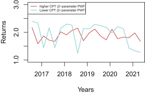
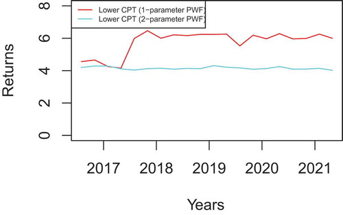
Figure 2, Figure 5, Figure 4 and Figure 7 suggest that portfolios consisting of one type of assets (exclusively, either cryptocurrencies or indices) with lower CPT values outperform those consisting of higher CPT values assets, irrespective of the decision weight (1- PWF and 2- PWF) used. Similarly, mixed assets portfolios from 1- PWF decision weight outperform those from 2- PWF, irrespective of CPT values.

Figure 2. Cryptocurrencies returns comparison (1—parameter PWF).

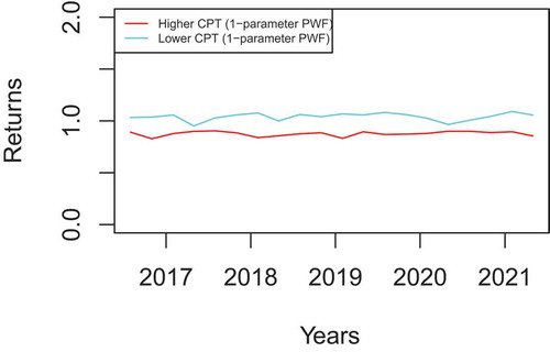
So, portfolios constructed from 1- PWF—lower CPT values appear to outperform the rest. Though this is true for cryptocurrencies and mixed portfolios, portfolios consisting of indices present a seemingly interchangeable performance across the entire study period, see Figures 3 and 6, suggesting a regime switching framework.

Figure 3. Indices returns comparison (1—parameter PWF).

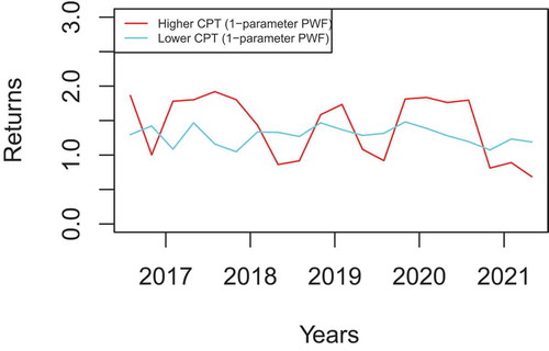
Figure 4. Mixed assets returns comparison (1—parameter PWF).

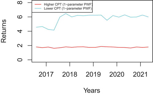
Figure 5. Cryptocurrencies returns comparison (2—parameter PWF).

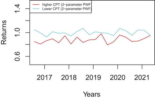
Figure 6. Indices returns comparison (2—parameter PWF).

Portfolios consisting of mixed assets achieved higher returns than those with single class assets; see Figure 4, Figure 7 and Figure 8. This is supported by Kajtazi and Moro (Kajtazi & Moro, 2019) who analyses the role of bitcoin in portfolios of European and Chinese assets. They reported that this combination generates benefits in terms of improvement of the returns, but it tends also to increase volatility. Our analysis reports similar observation with the CVaR in the last column of Table 19 higher than those in Table 17 and Table 18. This diversification strategy could be suitable for risk-seeking investors wanting to maximise their portfolio returns. This is supported by Andrianto and Diputra (Andrianto & Diputra, 2018) who conducted a study to examine the effects of cryptocurrency on the investment portfolio and found that cryptocurrency enhances portfolio performance. They also noted that portfolios containing cryptocurrencies seem to beat the quality of the S&P 500 and Dow Jones indices.

Table 17. Risk (CVaR) and Returns for Indices and Cryptocurrencies with higher and lower CPT values (1—parameter PWF)

	Crypto with higher CPT		Crypto with lower CPT		Indices with higher CPT		Indices with lower CPT
Rebal. Periods	CVaR	Return	CVaR	Return	CVaR	Return	CVaR	Return
P1	0.0341	0.8664	0.0101	0.9753	1	1.6392	1	1.8530
P2	0.0025	0.8909	0.0358	1.0335	1	1.8625	0.1071	1.2965
P3	0.0285	0.8278	0.0020	1.0366	0.2023	1.0029	0.2000	1.4215
P4	0.0110	0.8780	0.0091	1.0573	1	1.7805	0.0931	1.0844
P5	0.0060	0.8993	0.0002	0.9517	1	1.8017	0.0466	1.4665
P6	0.0686	0.9043	0.0077	1.0292	1	1.9193	0.0709	1.1593
P7	0.0070	0.8847	0.0556	1.0580	1	1.8038	0.0141	1.0471
P8	0.0315	0.8390	0.0075	1.0767	1	1.4327	0.3833	1.3339
P9	0.0257	0.8561	0.0107	0.9997	0.1690	0.8617	0.0378	1.3292
P10	0.0343	0.8757	0.0270	1.0620	0.2147	0.9164	0.2754	1.2687
P11	0.0304	0.8858	0.0038	1.0403	1	1.5853	0.1481	1.4673
P12	0.0138	0.8317	0.0531	1.0677	1	1.7337	0.1465	1.3675
P13	0.0057	0.8949	0.0598	1.0572	0.3756	1.0814	0.0099	1.2838
P14	0.0079	0.8692	0.0072	1.0819	0.1762	0.9185	0.2231	1.3151
P15	0.0054	0.8722	0.0308	1.0610	1	1.8125	0.2943	1.4815
P16	0.0067	0.8795	0.0218	1.0257	1	1.8354	0.0402	1.3872
P17	0.0368	0.9001	0.0596	0.9653	1	1.7616	0.0622	1.2803
P18	0.0172	0.9003	0.0180	1.0065	1	1.7957	0.0678	1.1947
P19	0.0276	0.8875	0.0758	1.0442	0.0114	0.8108	0.1149	1.0732
P20	0.0410	0.8952	0.0548	1.0909	0.1853	0.8899	0.0768	1.2326
P21	0.0041	0.8552	0.0638	1.0565	0.0004	0.6855	0.0190	1.1893

Table 18. Risk (CVaR) and Returns for Indices and Cryptocurrencies with higher and lower CPT values (2-parameter PWF)

	Crypto with higher CPT		Crypto with lower CPT		Indices with higher CPT		Indices with lower CPT
Rebal. Periods	CVaR	Return	CVaR	Return	CVaR	Return	CVaR	Return
P1	0.1042	0.7881	0.0060	1.0080	1	1.7557	0.1183	1.3473
P2	0.0824	0.8474	0.0044	1.0475	1	2.1655	1	2.3967
P3	0.0527	0.8070	0.0437	0.9933	1	1.5857	1	2.3321
P4	0.0229	0.8646	0.0143	0.9258	1	1.8669	0.0537	1.4519
P5	0.0403	0.8940	0.0155	1.0127	1	1.7140	1	2.1588
P6	0.0282	0.8280	0.0478	0.9876	1	1.6713	0.1178	1.4506
P7	0.1382	0.9460	0.0559	0.9934	1	2.0161	1	2.1435
P8	0.0854	0.8084	0.0006	0.9426	1	1.9069	1	2.2973
P9	0.0240	0.9223	0.02259	1.0157	1	2.0670	1	2.2596
P10	0.0531	0.8333	0.0818	1.0675	1	2.1485	0.0748	1.2441
P11	0.0806	0.8767	0.0074	0.9631	1	1.6954	1	2.1399
P12	0.1061	0.8833	0.0435	1.0117	1	1.9770	1	2.1193
P13	0.1376	0.9798	0.0237	0.9974	1	2.1174	1	2.2854
P14	0.0530	0.7921	0.0442	0.9880	1	1.8668	1	2.2441
P15	0.0340	0.8433	0.0065	0.9486	1	1.7288	1	2.1785
P16	0.1648	0.9591	0.0763	1.0676	1	2.1095	1	1.9792
P17	0.0548	0.9225	0.0999	1.0325	1	1.7686	1	2.2020
P18	0.0428	0.8502	0.0647	0.9529	1	1.8247	1	2.1315
P19	0.0233	0.8561	0.0319	1.0435	1	1.8063	0.1902	1.4240
P20	0.0445	0.8996	0.0167	1.0397	1	1.9764	0.1907	1.3293
P21	0.0764	0.9482	0.0333	0.9566	1	1.6763	0.0319	1.2778

Table 19. Returns for mixed assets portfolios with lower and higher CPT (1 & 2—parameter PWF)

	Lower CPT (2-para. PWF)	Lower CPT (1-para. PWF)	Higher CPT (1-para. PWF)	Higher CPT (2-para. PWF)
Rebal. Periods	Returns	Returns	Returns	Returns	CVaR
P1	4.3514	4.4016	1.7426	1.6002	1
P2	4.1953	4.5573	1.8007	1.5203	1
P3	4.2858	4.6551	1.7016	1.5680	1
P4	4.2817	4.2527	1.7878	1.5891	1
P5	4.1086	4.1498	1.6122	1.5695	1
P6	4.0352	5.9841	1.6887	1.5042	1
P7	4.1221	6.4634	1.8128	1.6034	1
P8	4.1477	6.0016	1.7488	1.5604	1
P9	4.0897	6.2113	1.8101	1.5181	1
P10	4.1392	6.1629	1.8215	1.5455	1
P11	4.1215	6.2394	1.7336	1.5476	1
P12	4.3087	6.2375	1.7389	1.5723	1
P13	4.2111	6.2557	1.8666	1.5094	1
P14	4.1675	5.5291	1.8218	1.5944	1
P15	4.0871	6.1862	1.7963	1.5171	1
P16	4.1282	5.9678	1.7380	1.4971	1
P17	4.2530	6.2844	1.7260	1.4475	1
P18	4.0906	5.9601	1.6520	1.4875	1
P19	4.0982	5.9865	1.7959	1.5503	1
P20	4.1426	6.2540	1.7315	1.4945	1
P21	4.0195	5.9997	1.7900	1.5517	1

Figure 7. Mixed assets returns comparison (2—parameter PWF).

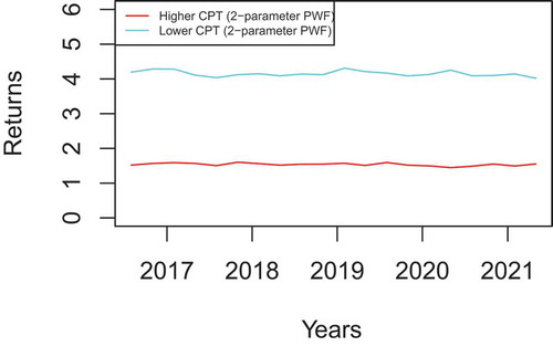
Figure 8. Returns comparison for mixed assets with lower CPT values (1& 2—parameter PWF).

5. Conclusion

Based on the Cumulative Prospect Theory (CPT) values, fourteen (14) portfolios have been formed. The results showed that portfolios consisting of assets (cryptocurrencies or mixed) with extremely lower CPT outperform those with higher CPT values, both 1—parameter PWF and 2—parameter PWF. Moreover, portfolios consisting of mixed assets (cryptocurrencies and indices) generates benefits in terms of improvement of the returns, but it tends also to increase volatility.

Portfolios consisting of indices only, present a seemingly interchangeable performance across the entire study period. This periodic-like behaviour suggests a regime switching approach. This will be the focus of our future investigation. For practical use of this study, we may recommend the one parameter behavioural selection criteria. Also, risk-seekers investors may consider including cryptocurrencies in their portfolio for higher returns.

Cover Image

Source: Author.

Acknowledgements

The second author thanks the AAMP Programme of the University of Johannesburg for their financial support to carry out this study. He also thanks the Research Center of AIMS-Cameroon for hosting him during the writing and revision of this article.

Additional information

Funding

The authors received no direct funding for this research.

Notes on contributors

Kofi Agyarko Ababio

Kofi Agyarko Ababio research interest focuses on Financial/Statistical Econometrics, Asset Selection, Portfolio Diversification and Optimisation, Behavioural Economics/Finance, and Decision Science.

Jules Clement Mba

Jules Clement Mba research interest comprises Portfolio selection and optimization, Risk management, Machine learning, cryptocurrencies.

Ur Koumba

Ur Koumba research interest focuses on Operator theory and its applications in optimization, Mathematical modeling and Financial market theory.

References

- Ababio, K. A. (2019). Behavioural portfolio selection and optimisation: Equities versus cryptocurrencies. Journal of African Business, 21(2), 1–27. DOI: 10.1080/15228916.2019.1625018
- Abdellaoui, M. (2000). Parameter-free elicitation of utility and probability weighting functions. Management Science, 46(11), 1497–1512. https://doi.org/10.1287/mnsc.46.11.1497.12080
- Andersen, S., Harrison, G. W., & Rutstrom, E. E. (2006). Choice behaviour, asset integration and natural reference points, Technical report, Working Paper 06.
- Andrianto, Y., & Diputra, Y. (2018). The effect of Cryptocurrency on investment portfolio effectiveness. Journal of Finance and Accounting, 6(5), 229–238.
- Bekiros, D., Hernandez, J. A., Hammoudeh, S., & Nguyen, D. K. (2015). Multivariate dependence risk and portfolio optimization: An application to mining stock portfolios. International Journal of Minerals Policy and Economics, 46(2), 1–11.
- Breymann, W., Dias, A., & Embrechts, P. (2003). Dependence structures for multivariate high-frequency data in finance. Quantitative Finance, 3(1), 1–14. https://doi.org/10.1080/713666155
- Brunnermeier, M. K. (2009). Deciphering the 2007–08 liquidity and credit crunch. Journal of Economic Perspectives, 23(1), 77–100. https://doi.org/10.1257/jep.23.1.77
- Camerer, C. F. (2000). Prospect theory in thewild: Evidence from the field. In D. Kahneman & A. Tversky (Eds.), Choices, values, and frames (pp. 288–300). Cambridge University Press.
- Donkers, B., Melenberg, B., & Van Soest, A. (2001). Estimating risk attitudes using lotteries: A large sample approach. Journal of Risk and Uncertainty, 22(2), 165–195. https://doi.org/10.1023/A:1011109625844
- Embrechts, P., McNeil, A., & Straumann, D. (2002). Correlation and dependence in risk management: Properties and pitfalls. In M. Dempster (Ed.), Risk management: Value at risk and beyond (pp. 176–223). Cambridge University Press.
- Fang, H., & Fang, K. (2002). The meta–elliptical distributions with given marginals. Journal of Multivariate Analysis, 82(1), 1–16. https://doi.org/10.1006/jmva.2001.2017
- Fehr-Duda, H., De Gennaro, M., & Schubert, R. (2006). Gender, financial risk, and probability weights. Theory and Decision, 60(2–3), 283–313. https://doi.org/10.1007/s11238-005-4590-0
- Florackis, C., Kontonikas, A., & Kostakis, A. (2014). Stock market liquidity and macro - liquidity shocks: Evidence from the 2007–2009 financial crisis. Journal of International Money and Finance, 44, 97–117. https://doi.org/10.1016/j.jimonfin.2014.02.002
- Gârleanu, N., & Pedersen, L. (2013). Dynamic trading with predictable returns and transaction costs. The Journal of Finance, 68(6), 2309–2340. https://doi.org/10.1111/jofi.12080
- Goldstein, W. M., & Einhorn, H. J. (1987). Expression theory and the preference reversal phenomena. Psychological Review, 94(2), 236. https://doi.org/10.1037/0033-295X.94.2.236
- Harrison, G. W., & Rutström, E. E. (2009). Expected utility theory and prospect theory: One wedding and a decent funeral. Experimental Economics, 12(2), 133–158. https://doi.org/10.1007/s10683-008-9203-7
- Holland, J. H. (1975). Adaptation in natural artificial systems. University of Michigan Press.
- Kahneman, D., & Tversky, A. (1979). Prospect theory: An analysis of decision under risk. Econometrica, 47(2), 263–291. https://doi.org/10.2307/1914185
- Kajtazi, A., & Moro, A. (2019). The role of bitcoin in well diversified portfolios: A comparative global study. International Review of Financial Analysis, 61, 143–157. https://doi.org/10.1016/j.irfa.2018.10.003
- Mba, J. C., Pindza, E., & Koumba, U. (2018). A differential evolution copula-based approach for a multi-period cryptocurrency portfolio optimization. Financial Markets and Portfolio Management, 32(4), 399–418. https://doi.org/10.1007/s11408-018-0320-9
- Moshirian, F. (2011). The global financial crisis and the evolution of markets institutions and regulation. Journal of Banking and Finance, 35(3), 502–511. https://doi.org/10.1016/j.jbankfin.2010.08.010
- Nystrup, P., Madsen, H., & Lindström, E. (2016). Dynamic portfolio optimization across hidden market regimes. Working paper, Technical University of Denmark.
- Omane-Adjepong, M., Ababio, K. A., & Alagidede, P. (2019). Time-frequency analysis of behaviourally classified financial asset markets. Research in International Business and Finance.
- Prelec, D. (1998). The probability weighting function. Econometrica.
- Price, K., Storn, R. M., & Lampinen, J. A. (2006). Differential evolution: A practical approach to global optimization. Springer Science & Business Media.
- Simo-Kengne, B. D., Ababio, K. A., Mba, J., & Koumba, U. (2018). Behavioural portfolio selection and optimisation: An application to international stocks. Financial Markets and Portfolio Management, 32(3), 311–328. https://doi.org/10.1007/s11408-018-0313-8
- Sklar, A. (1959). Fonctions de répartition à n dimensions et leurs marges. Publications De l’Institut De Statistique De l’Université De Paris, 8, 229–231.
- Storn, R., & Price, K. (1997). Differential evolution – A simple and efficient heuristic for global optimization over continuous spaces. Journal of Global Optimization, 11(4), 341–359. https://doi.org/10.1023/A:1008202821328
- Tu, Q. (2005). Empirical analysis of time preferences and risk aversion, Technical report, Tilburg University, School of Economics and Management.
- Tversky, A., & Kahneman, D. (1992). Advances in prospect theory: Cumulative representation of uncertainty. Journal of Risk and Uncertainty, 5(4), 297–323. https://doi.org/10.1007/BF00122574
- Yollin, G. (2009). R tools for portfolio optimization. Presentation at R/Finance conference 2009.