Does trade openness affect economic growth in India? Evidence from threshold cointegration with asymmetric adjustment

Abstract

This paper investigates the long-run equilibrium relationship between economic growth and trade openness in India during the period 1960–2018 using the asymmetric error-correction model with threshold cointegration. To evaluate the robustness impact of trade openness on economic growth under different regimes, we divide the full sample period into two sub-periods, i.e., pre-trade reforms period 1960–1990, and post-trade reforms period 1991–2018. The study indeed confirms the evidence of asymmetric cointegration between economic growth and trade openness in India during the period under evaluation and over the different sub-periods. The estimated asymmetric error-correction model exhibits a different speed of adjustment in trade openness in response to positive and negative economic growth shocks in the short-run. More specifically, during the pre-reforms period, deviations from the long-run equilibrium due to a relative increase in economic growth have a lower speed of adjustment in comparison to deviations caused by a corresponding decrease in economic growth in India.

Keywords:

• economic growth
• trade openness
• threshold cointegration
• error correction mechanism

Jel:

• C32
• F62
• O47

PUBLIC INTEREST STATEMENT

This paper investigates the linear vs. non-linear relationship between trade openness and economic growth in India during the period 1960–2018. Furthermore, to do the sensitivity analysis of the results, we divide the full-sample into two sub-samples, i.e., pre-trade and post-trade reforms period based on the trade reforms in India in 1991. Empirical results exhibit that trade openness and economic growth are asymmetrically related to each other during the period under study and over the pre-trade and post-trade reforms period. Our results indicate that the speed of adjustment in trade openness response to changes in economic growth shocks in the short-run has varied across different sub-periods of the analysis. More specifically, empirical results exhibit that during the post-trade reforms period, economic growth response to positive deviations in trade openness is significantly slow, such that it takes approximately 38 months to digest fully.

1. Introduction

The importance of trade openness has been gaining momentum since the time of globalization. Each country is now giving priority towards the new strategies to assimilate the domestic economy to the world economies through the opening of its trade through different channels. The trade openness has been regularly contributing to economic growth in both developing and developed countries in less or to a greater extent. On this backdrop, theoretical models show that trade openness facilitates the efficient allocation of resources through comparative advantage, leading to increased income levels (Grossman & Helpman, 1991). However, the endogenous growth model postulates that economic growth due to trade varies depending on whether the force of comparative advantage orientates the economy’s resources such that it generates economic growth or away from such activities. Theories suggest that, due to technological or financial constraints, less-developed countries may lack the social and technical capability which is required to adopt technologies developed in advanced economies. Therefore, despite its positive effect on growth, some theoretical studies claim that trade openness may hamper economic growth, where technological innovations or learning by doing are primarily exhausted, or where selective protection may foster faster technological advances (Lucas, 1988).

The relationship between economic growth and trade openness has been inconclusive and theoretically controversial. The conventional wisdom predicts a growth-enhancing effect of trade. In contrast, the recent developments suggest that trade openness is not always a growth-enhancing effect such that it benefits the economic growth of countries. Even increased international trade can generate economic growth by facilitating the diffusion of knowledge and technology from foreign direct investment (FDI) or through direct import of high tech goods (Almeida & Fernandes, 2008). Trade facilitates integration with global trade with the sources of innovation and enhances gain from FDI. The trade openness allows economies to expand production, increasing returns to scale, and economics of specialization (Bond et al., 2005). Grossman and Helpman (1991) show that trade openness improves transfers of new technologies, facilitating technological progress and productivity, and these benefits depend upon the degree of trade openness. Therefore, trade openness reduces the misallocation of resources in the short-run, whereas it facilitates the transfer of technological development in the long-run. Hence, in the expectation of economic growth stimulation, many developing countries have been implemented the trade liberalization policies in different phases of time.

The empirical evidence of trade openness impact on economic growth is still inconclusive and mixed (Yanikkaya (2003); and Rodriguez and Rodrik (2001).¹ From the empirical evidence perspective, there are two groups of studies. First, groups of studies have justified the significance of trade openness and its favorable impact on economic growth (Bahmani-Oskooee & Niroomand, 1999; Das & Paul, 2011; Harrison, 1996; Lee et al., 2004). A study by Marelli and Signorelli (2011) concluded that trade openness has a positive effect on economic growth. In contrast, Hye and Lau (2014) find that trade openness has a positive impact on economic growth in the short-run, but it harms in the long-run. On the other hand, the second group of studies has found that trade openness harms economic growth (Gries et al., 2009; Hye et al., 2014; Zahonogo, 2016). Trade openness has a positive impact on economic growth across developed countries, and it harms developing countries (Kim et al., 2011; Vlastou, 2010). But at the same time, other sets of studies suggest that there is no significant relationship between trade openness and economic growth (Eriṣ & Ulaṣan, 2013; Menyah et al., 2014; Ulaşan, 2014; Yanikkaya, 2003). Using data from 131 developed and developing countries, Manole and Spatareanu (2010) find that trade protection is associated with higher per capita income countries. Moreover, few studies have examined this controversial issue in the Indian context since after the trade labialization in the 1990 s (Agrawal, 2015; Chandra, 2003; Goldberg et al., 2010; Sharma & Panagiotidis, 2005). Therefore, the relationship between economic growth and trade openness is still an open question in development studies and provide scope for further extensive empirical analysis. However, the relationship between economic growth and trade openness differs from country to country.

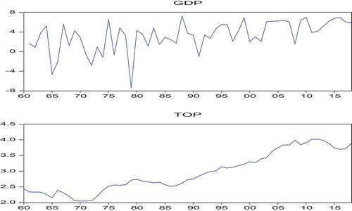
The Indian economy was facing the problems of declining foreign exchange, growing imports without a matching rise in exports, and high inflation during 1980. India started its trade liberalization policies of export-led growth strategy in 1991 due to a financial crisis and pressure from international organizations like the World Bank and International Monetary Fund (IMF). The new trade liberalization policy in 1991 had coupled with a lot of reforms step to reduce the import duties, opened the public sector for the private players, devalued the Indian currency to increase the export, and alleviate the adverse Balance of Payment (BOP) situation. Moreover, trade share in GDP has been declining before the 1990 s. However, after the 2000 s, trade share in GDP shows consistently increasing due to the rapid dismantling of tariff and other measures to improve the export-led trade in India. The trade share in GDP has been continuously rising after the 2000 s, because of the positive consequences of trade liberalization policies initiated by the Indian government in the year 1991. To boost the trade share in GDP and export competitiveness, India has adopted a series of trade policy reforms with financial sector reforms after the 1990 s. Similarly, GDP per capita in India has been experiencing fluctuating trends before the initiation of trade reforms and financial liberalization policies during 1980; however, it is consistently rising after the 1990 s. The direction of trade openness (TOP) and economic growth (GDP) in India over the period 1960–2018 has been presented in Figure 1.

Figure 1 shows that economic growth measured by GDP per capita has been volatile and shows negative growth during the period 1960–1980.² Although, the trends show negative growth and quite oscillating; however, after economic reforms in 1991, the growth rate has been changed dramatically and moves upwards. Therefore, due to various problems like BOP and macroeconomic instability coupled with stagnation and high inflation, the Indian GDP per-capita growth rate shows non-linear. Nevertheless, trade share in GDP (trade openness) has been increasing since the trade liberalization in India after 1990. The trade share in GDP has increased significantly after 2000. Also, this is almost reached from 11 percent of GDP in 1960 to close to 50 percent of GDP in the year 2018. Therefore, this indicates that the Indian government and policymakers have taken massive steps to reform the external sector, specifically focusing on Indian manufacturing industries to boost the export sector. This prima-facie evidence suggests that there are specific possible linkages between economic growth and trade openness in India, and the connections are non-linear. Furthermore, as there is a series of fluctuations between economic growth and trade openness in India, so, the possibility of non-linearity is quite observable.

Figure 1. The trend of economic growth (GDP) and trade openness (TOP) in India over the period 1960–2018.

The main contributions to this research to the existing literature related to the transmission mechanism between trade openness and economic growth are discussed below. This study contributes to research by assessing whether the relationship between trade and economic growth is non-linear. This distinction is essential, as various theoretical models and empirical results have suggested that the effect of trade openness on economic growth is linear. Moreover, this is a significant departure from previous studies who firmly believe that the relationship between economic growth and trade openness are symmetrical. Furthermore, India is considered to be the fastest-growing emerging economy in the world. As of 2019, India is 5th largest country of the world, and on purchasing power parity (PPP) basis, India stands at 3rd place. In 2017–18, India’s economy was 9.448 USD trillion (PPP) and accounted for a 7.45% share of world GDP (PPP). Since after independence in 1947, and specifically, after 1960 in this study, how trade share contributed to the Indian GDP would be quite interesting to examine this issue. Therefore, this motivates the researchers to explore the possible transmission mechanism between these two driving forces in India. Therefore, taking into the significance of India’s position at the world level, it is worthwhile to examine the possible transmission mechanism between economic growth and trade openness in India and their non-linear adjustment. Secondly, another notable attempt to investigate the direction of causality and asymmetric speed of adjustment between economic growth and trade openness in a non-linear framework could give a clear indication for the time path of adjustment in the future. In sum, the application of asymmetric adjustment between the variables in our study, supposed to be a better approach than the previous methodology of the traditional linear adjustment method.

The rest of the paper is structured as follows. Section 2 summarizes the review of the literature. Section 3 discusses the definition and sources of data used and methodology. Section 4 presents empirical results and their interpretations. Finally, Section 5 discusses the concluding remarks.

2. Literature review

The relationship between trade openness and economic growth is still an open question in the economic growth and development literature. Traditional trade theory shows that growth gains from trade openness at the country level are viable through specialization, innovation in investment, improvement in productivity, and efficient resource allocation. The role of trade policy in economic development has been considered as a vital matter of debate in the development literature. Theoretical growth studies suggest a complex and ambiguous relationship between trade openness and economic growth. Furthermore, academic growth literature has given attention to the relationship between trade policies and economic growth rather than the relationship between trade volumes and economic growth (Yanikkaya, 2003). Therefore, Yanikkaya (2003) suggests that the relationship between trade barriers and growth cannot be directly applied to the effects of changes in trade volumes on economic growth. However, these two concepts, trade volumes and trade restrictions, are very much closely related. Besides, their relationship with economic growth may differ considerably because of several other factors that affect a country’s external sectors, such as geographical factors, country size, and income (Rodriguez & Rodrik, 2001). Nevertheless, researchers, today are facing a severe problem because of the lack of a clear definition of what is meant by “trade liberalization” or “trade openness.” Therefore, over time, the definition of openness has been developed considerably from one extreme to another. Krueger (1978) has discussed how trade liberalization can be achieved by employing policies, which reduces the biases against the export sector. She suggests that one country can be an open economy by applying a favorable exchange rate policy towards its export sectors and, at the same time, use trade barriers to protect its importing industry from encouraging import substitution.

There is even a large number of empirical studies that have used cross-country growth regressions to test the endogenous growth theory to examine the link between trade openness and economic growth (Edwards, 1993; Rodriguez & Rodrik, 2001; Temple, 1999). Different researchers have used various measures to examine the effects of trade openness on economic growth (Sachs et al., 1995; Yanikkaya, 2003). Anderson and Neary (1992) have developed a “trade restrictiveness index”, which in principle incorporates the effects of both tariffs and non-tariff barriers. However, due to its non-availability in many large samples of countries, some existing studies have used the available data to measure trade openness, and some other studies have constructed indices (Dollar, 1992; Leamer, 1988; Sachs et al., 1995). A large number of studies have used trade shares in GDP (exports and imports divided by GDP) and found a positive relationship between trade openness and economic growth (Frankel & Romer, 1999; Harrison, 1996; Irwin & Terviö, 2002). Furthermore, empirical evidence shows that in the long run, more export-oriented countries experience higher economic growth (Chang et al., 2009; Dollar & Kraay, 2004; Freund & Bolaky, 2008; Lee et al., 2004).

Birinci (2013) investigated the relationship between trade openness and economic growth in the OECD countries and found bidirectional causality between trade openness and economic growth. In the case of the Algerian economy, Hamdi and Sbia (2013) found unidirectional causality from trade openness to economic growth in the short-and long-run. Liu et al. (1997) find the bidirectional causality between trade openness and economic growth in China. Jin (2000) has examined the nexus between trade openness and economic growth in East Asian countries, and find the weak evidence of trade openness effects on long-run economic growth. In another study, Jin (2004) find that trade openness has a positive impact on economic growth in the eastern coastal regions in China. In contrast, he finds that trade openness harms GDP growth in the island regions in China. Lee et al. (2004) also find a positive effect of trade openness on economic growth. Using the ARDL approach, Hye and Lau (2014) evaluate the nexus between trade openness and economic growth in India over the period 1971–2009. They find that trade openness has a positive impact on economic growth in the short-run and detrimental in the long run. Besides, the Granger causality test shows the unidirectional causality runs from trade openness to economic growth in the short-run as well as in the long-run. Moreover, empirical studies have found a possible two-way causality in the trade-growth link, which suggests that more trade may be linked with higher-income countries. Thus, it indicates that countries with higher income may be better able to afford the infrastructure conducive to trade and demand more traded goods (Kim & Lin, 2009).

Different scholars have used the trade openness indicators to measure economic growth in different ways, like measures based on trade restrictions and distortions. The different way of measuring openness is closely linked to the economic growth rate. Therefore, it is likely that all measures of openness are jointly endogenous with economic growth, which may cause biases in the estimation because of simultaneity or reverse causality (Lee et al., 2004). To test the long-run relationship between economic growth and trade openness, most of the earlier studies have used the linear cointegration approaches of Engle and Granger (1987) and Johansen and Juselius (1990). However, these studies are neither correct nor accurate in the presence of transaction costs and asymmetries in price transmission (Balke & Fomby, 1997). Balke and Fomby (1997) criticize all previous studies that assume symmetric adjustments towards the long-run equilibrium between trade openness and economic growth. Moreover, empirical literature suffers from severe methodological laxity in the advent of a newly developed and most robust model of threshold cointegration, which in general assumes asymmetric adjustment, unlike symmetric adjustment towards the long-run equilibrium analysis in time series data.

Balke and Fomby (1997) proposed a threshold cointegration analysis that assumes the adjustment towards the long-run equilibrium holds when the deviation from the equilibrium exceeds some threshold level (Stigler, 2012). Eventually, instead of considering the symmetric adjustments, we move further to evaluate the asymmetric adjustment between trade openness and economic growth in India using the TAR and MTAR models.³ The TAR and MTAR models allow asymmetric adjustment between variables while reverting to long-run equilibrium following a shock in the short-run (Balke & Fomby, 1997; Enders & Granger, 1998; Enders & Siklos, 2001). Therefore, the research complements the literature on trade and growth by providing new country-level evidence that considers the threshold effects of trade openness on economic growth in India. Moreover, rather than just thinking about the direct impact of trade on economic growth, this study goes further and explores the nonlinear long-run equilibrium relationship between trade openness and economic growth, and measures the asymmetrical adjustment from their long-run equilibrium path. The study has used the APT package (Sun, 2011) for the estimation of threshold cointegration and asymmetric error correction model (AECM).

3. Data and methodology

3.1. Data

The study uses annual time series data from 1960–2018 to construct the variables of economic growth and trade openness in India. All data are obtained from the World Bank, world development indicators online data set (World Bank, 2018). Followed by previous studies (Al-Shayeb & Hatemi-J, 2016; Le Goff & Singh, 2014; Irwin & Terviö, 2002; Jouini, 2015), we have used the standard measurement of trade openness (TOP), i.e., it is constructed by adding exports and imports divided by gross domestic product. Similarly, followed by previous studies (Al-Shayeb & Hatemi-J, 2016; Zahonogo, 2016), our measurement of economic growth (GDP) is constructed by the log-difference of real GDP per-capita $(\mathrm{\Delta }GD{P}_t$).⁴

3.2. Methodology

We follow three familiar econometrics steps to investigate the impact of trade openness on economic growth in India. Initially, we follow the unit root test to check the presence or absence of unit root in the data. Followed by a unit root test, we have tested the liner vs. non-linear cointegration between the trade openness and economic growth in India. Finally, we have examined the asymmetric long-run adjustment between the two variables by applying the asymmetric error-correction model (AECM). These three standard econometric procedures are discussed below.

3.2.1. Unit root test in the presence of structural breaks

Unit root tests in time series data play a very prominent role in determining the order of integration of time series variables. The most celebrated one is the augmented Dickey-Fuller (ADF) test, which does not consider the presence of structural breaks in the macroeconomics data. Hence, the ADF tests are biased towards the non-rejection of the null-hypothesis (Perron, 1989) in the presence of structural break. Therefore, the study has applied the unit root test developed by Perron and Vogelsang (1992) to find out the existence of a possible one structural break in the data. The “additive outlier” (AO), models consider break occur immediately, while the second, called as the “innovational outlier” (IO), models consider break as evolving more slowly over time. The selection of AO vs. IO depends on the dynamics of the transition path following a break (Perron & Vogelsang, 1992). The AO model has been estimated with the help of two-step procedures. In the first step, it removes the deterministic part of the series by estimating the following regression, which is as follows:

(2) $y_{\mathrm{t}}=\mu +\delta \mathrm{D}{\mathrm{U}}_{\mathrm{t}}+{\eta }_{\mathrm{t}}$(2)

where $D{U}_t=0$ if $t\le TB$ (the break date) and is one otherwise.⁵ The AO model allows for a change in the mean of a series ${\left\{y_t\right\}}_1^T$, say at time TB (1< TB < T).

The estimated residuals in the next step are used to test for the presence of a unit-root by estimating the following equation.

(2) ${\eta }_{\mathrm{t}}=\sum _{\mathrm{i}=0}^{\mathrm{k}}{\omega }_{\mathrm{i}}\mathrm{D}\mathrm{T}{\mathrm{B}}_{\mathrm{t}-\mathrm{i}}+\rho {\eta }_{\mathrm{t}-1}+\sum _{\mathrm{i}=0}^{\mathrm{k}}{\mathrm{C}}_{\mathrm{i}}\mathrm{\Delta }{\eta }_{\mathrm{t}-1}+{\epsilon }_{\mathrm{t}}$(2)

where ${\eta }_t$ is the residuals obtained from Equation (1), and TB considered to be the break date, DTB is a pulse variable that takes the value one if $DT{B}_t=1$ for t = TB+1 and zero, otherwise. Equation (1) and Equation (2)(2) $y_{\mathrm{t}}=\mu +\delta \mathrm{D}{\mathrm{U}}_{\mathrm{t}}+{\eta }_{\mathrm{t}}$(2) are estimated by OLS, which takes into consideration each break year TB = k + 2, …., T-1, where T presents the number of observations, and k presents the truncation lag parameter. If the t-statistic on $\rho$ becomes non-zero (significantly different from zero), the null hypothesis of a unit root will be rejected. In this situation, variable (for instance, trade openness) will be a stationary time series around a structural break. The break would bring temporary changes in trade openness. Against this, if the t-statistic on $\rho$ is not significantly different from zero, the trade openness would be a non-stationary time series, and any sudden break would have permanent effects on the long-run level of trade openness.

3.2.2. Unit roots in the presence of double structural breaks

Most of the macroeconomic variables do not consider one break. So, it is essential to check for double structural breaks in the variables. For more than one break, Clemente, Montanes, and Reyes (CMR) (1998) test are applied to both variables in this study. Clemente et al. (1998) estimate the following regression to examine the unit root in the presence of more than one structural break by considering Perron and Vogelsang (1992) procedure. So, Equations (1) and (2(2) $y_{\mathrm{t}}=\mu +\delta \mathrm{D}{\mathrm{U}}_{\mathrm{t}}+{\eta }_{\mathrm{t}}$(2) ) can be changed to,

(3) $y_t=\mu +{\delta }_{1}D{U}_{1t}+{\delta }_{2}D{U}_{2t}+{\eta }_t$(3)

(4) ${\eta }_t=\sum _{i=0}^k{\omega }_{1i}DT{B}_{1t-i}+\sum _{i=0}^k{\omega }_{2i}DT{B}_{2t-i}+\rho {\eta }_{t-1}+\sum _{i=1}^k{C}_i{\eta }_{t-i}+{\epsilon }_t$(4)

where $D{U}_{jt}=1ift>T{B}_j\left(j=1,2\right)$ and zero, otherwise. $DT{B}_{jt}$ becomes equal to one if $t=T{B}_j+1$and zero, otherwise. TB₁ and TB₂ are the periods where the mean is modified.

For the verification of the unit root null hypothesis, Equation (3)(3) $y_t=\mu +{\delta }_{1}D{U}_{1t}+{\delta }_{2}D{U}_{2t}+{\eta }_t$(3) has been initially estimated by OLS to remove the deterministic part of variables. Then the test is carried out by searching for the minimal Pseudo-t-ratio for $\rho =1$ hypothesis in Equation (4)(4) ${\eta }_t=\sum _{i=0}^k{\omega }_{1i}DT{B}_{1t-i}+\sum _{i=0}^k{\omega }_{2i}DT{B}_{2t-i}+\rho {\eta }_{t-1}+\sum _{i=1}^k{C}_i{\eta }_{t-i}+{\epsilon }_t$(4) for all breaks. If the t-statistic on $\rho$ is significantly different from zero, then the null hypothesis of a unit root is rejected. In this case, the variable exhibits two structural breaks. One shock on a break can cause temporary movements of the variable, but in the case of two breaks, it could cause permanent effects. Similarly, if the t-statistic on $\rho$ is not significantly different from zero, then the variable would be a non-stationary time series, and a sudden shock could have permanent impacts on the long-run level of the variable.

3.2.3. Threshold cointegration with asymmetric error-correction model

To examine the non-linear relationship between TOP and GDP in India, we have used the threshold cointegration, which is developed by Enders and Siklos (2001). Moreover, to examine the asymmetric cointegration relationship between trade openness and economic growth variables, the following steps are followed:

(5) $\mathrm{G}\mathrm{D}{\mathrm{P}}_{\mathrm{t}}={\alpha }_0+{\alpha }_1\mathrm{T}\mathrm{O}{\mathrm{P}}_{\mathrm{t}}+{ϵ}_{\mathrm{t}}$(5)

In the second step, two regime threshold models are estimated for the estimated error term${\widehat{ϵ}}_t$, which is explained by

(6) $\mathrm{\Delta }{\widehat{ϵ}}_{\mathrm{t}}={\rho }_1{\mathrm{I}}_{\mathrm{t}}{\widehat{ϵ}}_{\mathrm{t}-1}+{\rho }_2\left(1-{\mathrm{I}}_{\mathrm{t}}\right){\widehat{ϵ}}_{\mathrm{t}-1}+\sum _{\mathrm{i}=1}^{\mathrm{p}}{\mathrm{\varnothing }}_{\mathrm{i}}\mathrm{\Delta }{\widehat{ϵ}}_{\mathrm{t}-1}+{ϵ}_{\mathrm{t}}$(6)

where ${\rho }_1$, ${\rho }_2$ and ${\mathrm{\varnothing }}_i$ are coefficients; $p$ is the number of lags; ${ϵ}_t$ represents the white noise error term.

(7) ${\mathrm{I}}_{\mathrm{t}}=\left\{\begin{array}{c}1,if{\mathrm{Z}}_{\mathrm{t}-1}\ge \tau \\ 0,if{\mathrm{Z}}_{\mathrm{t}-1}<\tau \end{array}\right.$(7)

where $I_t$ is the Heaviside indicator, and $Z_{t-1}$ represents the threshold variable with two alternative definitions. In first, the threshold variable can be defined as the level of residuals, i.e., $Z_{t-1}={\widehat{ϵ}}_{t-1}$, which is called the threshold autoregressive (TAR) model.

(8) ${\mathrm{I}}_{\mathrm{t}}=\left\{\begin{array}{c}1,if\mathrm{\Delta }{\mathrm{Z}}_{\mathrm{t}-1}\ge \tau \\ 0,if\mathrm{\Delta }{\mathrm{Z}}_{\mathrm{t}-1}<\tau \end{array}\right.$(8)

Equation (8)(8) ${\mathrm{I}}_{\mathrm{t}}=\left\{\begin{array}{c}1,if\mathrm{\Delta }{\mathrm{Z}}_{\mathrm{t}-1}\ge \tau \\ 0,if\mathrm{\Delta }{\mathrm{Z}}_{\mathrm{t}-1}<\tau \end{array}\right.$(8) represents the momentum threshold autoregressive model (M-TAR), which captures more dynamics than the TAR model if $\mathrm{\Delta }{Z}_{t-1}$ is significantly different from zero. If ${\rho }_1={\rho }_2=\rho$, in Equation (6)(6) $\mathrm{\Delta }{\widehat{ϵ}}_{\mathrm{t}}={\rho }_1{\mathrm{I}}_{\mathrm{t}}{\widehat{ϵ}}_{\mathrm{t}-1}+{\rho }_2\left(1-{\mathrm{I}}_{\mathrm{t}}\right){\widehat{ϵ}}_{\mathrm{t}-1}+\sum _{\mathrm{i}=1}^{\mathrm{p}}{\mathrm{\varnothing }}_{\mathrm{i}}\mathrm{\Delta }{\widehat{ϵ}}_{\mathrm{t}-1}+{ϵ}_{\mathrm{t}}$(6) then it coincides with Engle and Granger (1987) symmetric adjustments. When ${\rho }_1={\rho }_2=\rho$ later, Equation (6)(6) $\mathrm{\Delta }{\widehat{ϵ}}_{\mathrm{t}}={\rho }_1{\mathrm{I}}_{\mathrm{t}}{\widehat{ϵ}}_{\mathrm{t}-1}+{\rho }_2\left(1-{\mathrm{I}}_{\mathrm{t}}\right){\widehat{ϵ}}_{\mathrm{t}-1}+\sum _{\mathrm{i}=1}^{\mathrm{p}}{\mathrm{\varnothing }}_{\mathrm{i}}\mathrm{\Delta }{\widehat{ϵ}}_{\mathrm{t}-1}+{ϵ}_{\mathrm{t}}$(6) can be rewritten as follows:

(9) $\mathrm{\Delta }{\widehat{ϵ}}_{\mathrm{t}}=\rho {\widehat{ϵ}}_{\mathrm{t}-1}+\sum _{\mathrm{i}=1}^{\mathrm{p}}{\mathrm{\varnothing }}_{\mathrm{i}}\mathrm{\Delta }{\widehat{ϵ}}_{\mathrm{t}-1}+{ϵ}_{\mathrm{t}}$(9)

From Equation (6)(6) $\mathrm{\Delta }{\widehat{ϵ}}_{\mathrm{t}}={\rho }_1{\mathrm{I}}_{\mathrm{t}}{\widehat{ϵ}}_{\mathrm{t}-1}+{\rho }_2\left(1-{\mathrm{I}}_{\mathrm{t}}\right){\widehat{ϵ}}_{\mathrm{t}-1}+\sum _{\mathrm{i}=1}^{\mathrm{p}}{\mathrm{\varnothing }}_{\mathrm{i}}\mathrm{\Delta }{\widehat{ϵ}}_{\mathrm{t}-1}+{ϵ}_{\mathrm{t}}$(6) , we can examine the asymmetric cointegration by testing the null hypothesis $(H_0:{\rho }_1={\rho }_2=0)$ of no cointegration. If the null hypothesis is rejected, then there is an existence of cointegration of either symmetric $(H_1:{\rho }_1={\rho }_2\ne 0)$ or asymmetric form $(H_1:{\rho }_1\ne {\rho }_2)$. If the null hypothesis is not rejected, then we can evaluate symmetric adjustment in the long-run equilibrium where the null hypothesis is tested as $H_0:{\rho }_1={\rho }_2$. Besides, if there is evidence of threshold cointegration, we have to follow the procedure of asymmetric error correction mechanism with a particular threshold value (TAR or M-TAR value). Furthermore, to estimate the asymmetric error-correction mechanism, the following equations can be formulated as follows:

(10) $\mathrm{\Delta }\mathrm{T}\mathrm{O}{\mathrm{P}}_{\mathrm{t}}={\theta }_{\mathrm{t}\mathrm{o}\mathrm{p}}+{\delta }_{\mathrm{t}\mathrm{o}\mathrm{p}}^{+}{\mathrm{E}}_{\mathrm{t}-1}^{+}+{\delta }_{\mathrm{t}\mathrm{o}\mathrm{p}}^{-}{\mathrm{E}}_{\mathrm{t}-1}^{-}+\sum _{\mathrm{j}=1}^{\mathrm{p}}{\alpha }_{\mathrm{t}\mathrm{o}\mathrm{p},\mathrm{j}}\mathrm{\Delta }\mathrm{T}\mathrm{O}{\mathrm{P}}_{\mathrm{t}-\mathrm{j}}+\sum _{\mathrm{j}=1}^{\mathrm{p}}{\beta }_{\mathrm{G}\mathrm{D}\mathrm{P},\mathrm{j}}\mathrm{\Delta }\mathrm{G}\mathrm{D}{\mathrm{P}}_{\mathrm{t}-\mathrm{j}}+{\vartheta }_{\mathrm{t}\mathrm{o}\mathrm{p},\mathrm{t}}$(10)

(11) $\mathrm{\Delta }\mathrm{G}\mathrm{D}{\mathrm{P}}_{\mathrm{t}}={\theta }_{\mathrm{G}\mathrm{D}\mathrm{P}}+{\delta }_{\mathrm{G}\mathrm{D}\mathrm{P}}^{+}{\mathrm{E}}_{\mathrm{t}-1}^{+}+{\delta }_{\mathrm{G}\mathrm{D}\mathrm{P}}^{-}{\mathrm{E}}_{\mathrm{t}-1}^{-}+\sum _{\mathrm{j}=1}^{\mathrm{p}}{\alpha }_{\mathrm{G}\mathrm{D}\mathrm{P},\mathrm{j}}\mathrm{\Delta }\mathrm{G}\mathrm{D}{\mathrm{P}}_{\mathrm{t}-\mathrm{j}}+\sum _{\mathrm{j}=1}^{\mathrm{p}}{\beta }_{\mathrm{t}\mathrm{o}\mathrm{p},\mathrm{j}}\mathrm{\Delta }\mathrm{T}\mathrm{O}{\mathrm{P}}_{\mathrm{t}-\mathrm{j}}+{\vartheta }_{\mathrm{G}\mathrm{D}\mathrm{P},\mathrm{t}}$(11)

where ${\mathrm{E}}_{\mathrm{t}-1}^{+}={\mathrm{I}}_{\mathrm{t}}{\hat{\xi }}_{\mathrm{t}-1}$ and ${\mathrm{E}}_{\mathrm{t}-1}^{-}=\left(1-{\mathrm{I}}_{\mathrm{t}}\right){\hat{\xi }}_{\mathrm{t}-1}$, and, ${\delta }^{+}$ represents the positive speed of adjustment coefficient, ${\delta }^{-}$ represents the negative speed of the adjustment coefficient. Besides, $\theta$ represents the constant, and ${\alpha }_j$and ${\beta }_j$represent the coefficients of the lagged difference of TOP and GDP, respectively. Also, $p$ represents the number of lags and ${\vartheta }_t$ denotes a white noise error term.

After modifying Equations (10)(10) $\mathrm{\Delta }\mathrm{T}\mathrm{O}{\mathrm{P}}_{\mathrm{t}}={\theta }_{\mathrm{t}\mathrm{o}\mathrm{p}}+{\delta }_{\mathrm{t}\mathrm{o}\mathrm{p}}^{+}{\mathrm{E}}_{\mathrm{t}-1}^{+}+{\delta }_{\mathrm{t}\mathrm{o}\mathrm{p}}^{-}{\mathrm{E}}_{\mathrm{t}-1}^{-}+\sum _{\mathrm{j}=1}^{\mathrm{p}}{\alpha }_{\mathrm{t}\mathrm{o}\mathrm{p},\mathrm{j}}\mathrm{\Delta }\mathrm{T}\mathrm{O}{\mathrm{P}}_{\mathrm{t}-\mathrm{j}}+\sum _{\mathrm{j}=1}^{\mathrm{p}}{\beta }_{\mathrm{G}\mathrm{D}\mathrm{P},\mathrm{j}}\mathrm{\Delta }\mathrm{G}\mathrm{D}{\mathrm{P}}_{\mathrm{t}-\mathrm{j}}+{\vartheta }_{\mathrm{t}\mathrm{o}\mathrm{p},\mathrm{t}}$(10) and (11(11) $\mathrm{\Delta }\mathrm{G}\mathrm{D}{\mathrm{P}}_{\mathrm{t}}={\theta }_{\mathrm{G}\mathrm{D}\mathrm{P}}+{\delta }_{\mathrm{G}\mathrm{D}\mathrm{P}}^{+}{\mathrm{E}}_{\mathrm{t}-1}^{+}+{\delta }_{\mathrm{G}\mathrm{D}\mathrm{P}}^{-}{\mathrm{E}}_{\mathrm{t}-1}^{-}+\sum _{\mathrm{j}=1}^{\mathrm{p}}{\alpha }_{\mathrm{G}\mathrm{D}\mathrm{P},\mathrm{j}}\mathrm{\Delta }\mathrm{G}\mathrm{D}{\mathrm{P}}_{\mathrm{t}-\mathrm{j}}+\sum _{\mathrm{j}=1}^{\mathrm{p}}{\beta }_{\mathrm{t}\mathrm{o}\mathrm{p},\mathrm{j}}\mathrm{\Delta }\mathrm{T}\mathrm{O}{\mathrm{P}}_{\mathrm{t}-\mathrm{j}}+{\vartheta }_{\mathrm{G}\mathrm{D}\mathrm{P},\mathrm{t}}$(11) ), we construct asymmetric and dynamic lag error-correction models, which are as follows:

(12) $\mathrm{\Delta }\mathrm{T}\mathrm{O}{\mathrm{P}}_{\mathrm{t}}={\theta }_{\mathrm{t}\mathrm{o}\mathrm{p}}+{\delta }_{\mathrm{t}\mathrm{o}\mathrm{p}}^{+}{\mathrm{E}}_{\mathrm{t}-1}^{+}+{\delta }_{\mathrm{t}\mathrm{o}\mathrm{p}}^{-}{\mathrm{E}}_{\mathrm{t}-1}^{-}+\sum _{\mathrm{j}=1}^{\mathrm{p}}{{\alpha }^{+}}_{\mathrm{t}\mathrm{o}\mathrm{p},\mathrm{j}}\mathrm{\Delta }{\mathrm{T}\mathrm{O}\mathrm{P}}_{\mathrm{t}-\mathrm{j}}^{+}+\sum _{\mathrm{j}=1}^{\mathrm{p}}{{\alpha }^{-}}_{\mathrm{t}\mathrm{o}\mathrm{p},\mathrm{j}}\mathrm{\Delta }{\mathrm{T}\mathrm{O}\mathrm{P}}_{\mathrm{t}-\mathrm{j}}^{-}+\sum _{\mathrm{j}=1}^{\mathrm{p}}{{\beta }^{+}}_{\mathrm{t}\mathrm{o}\mathrm{p},\mathrm{j}}\mathrm{\Delta }{\mathrm{G}\mathrm{D}\mathrm{P}}_{\mathrm{t}-\mathrm{j}}^{+}+\sum _{\mathrm{j}=1}^{\mathrm{p}}{{\beta }^{-}}_{\mathrm{t}\mathrm{o}\mathrm{p},\mathrm{j}}\mathrm{\Delta }{\mathrm{G}\mathrm{D}\mathrm{P}}_{\mathrm{t}-\mathrm{j}}^{-}+{\vartheta }_{\mathrm{t}\mathrm{o}\mathrm{p},\mathrm{t}}$(12)

(13) $\mathrm{\Delta }\mathrm{G}\mathrm{D}{\mathrm{P}}_{\mathrm{t}}={\theta }_{\mathrm{G}\mathrm{D}\mathrm{P}}+{\delta }_{\mathrm{G}\mathrm{D}\mathrm{P}}^{+}{\mathrm{E}}_{\mathrm{t}-1}^{+}+{\delta }_{\mathrm{G}\mathrm{D}\mathrm{P}}^{-}{\mathrm{E}}_{\mathrm{t}-1}^{-}+\sum _{\mathrm{j}=1}^{\mathrm{p}}{{\alpha }^{+}}_{\mathrm{G}\mathrm{D}\mathrm{P},\mathrm{j}}\mathrm{\Delta }{\mathrm{G}\mathrm{D}\mathrm{P}}_{\mathrm{t}-\mathrm{j}}^{+}+\sum _{\mathrm{j}=1}^{\mathrm{p}}{{\alpha }^{-}}_{\mathrm{G}\mathrm{D}\mathrm{P},\mathrm{j}}\mathrm{\Delta }{\mathrm{G}\mathrm{D}\mathrm{P}}_{\mathrm{t}-\mathrm{j}}^{-}+\sum _{\mathrm{j}=1}^{\mathrm{p}}{{\beta }^{+}}_{\mathrm{G}\mathrm{D}\mathrm{P},\mathrm{j}}\mathrm{\Delta }{\mathrm{T}\mathrm{O}\mathrm{P}}_{\mathrm{t}-\mathrm{j}}^{+}+\sum _{\mathrm{j}=1}^{\mathrm{p}}{{\beta }^{-}}_{\mathrm{G}\mathrm{D}\mathrm{P},\mathrm{j}}\mathrm{\Delta }{\mathrm{T}\mathrm{O}\mathrm{P}}_{\mathrm{t}-\mathrm{j}}^{-}+{\vartheta }_{\mathrm{G}\mathrm{D}\mathrm{P},\mathrm{t}}$(13)

where

$\mathrm{\Delta }{\mathrm{T}\mathrm{O}\mathrm{P}}_{\mathrm{t}-\mathrm{j}}^{+}=\left\{\begin{array}{c}\mathrm{T}\mathrm{O}{\mathrm{P}}_{\mathrm{t}-\mathrm{j}}-\mathrm{T}\mathrm{O}{\mathrm{P}}_{\mathrm{t}-\mathrm{j}-1,}\mathrm{T}\mathrm{O}{\mathrm{P}}_{\mathrm{t}-\mathrm{j}}\ge \mathrm{T}\mathrm{O}{\mathrm{P}}_{\mathrm{t}-\mathrm{j}-1,}\\ 0,\mathrm{T}\mathrm{O}{\mathrm{P}}_{\mathrm{t}-\mathrm{j}}<\mathrm{T}\mathrm{O}{\mathrm{P}}_{\mathrm{t}-\mathrm{j}-1,}\end{array}\right.$

$\mathrm{\Delta }{\mathrm{T}\mathrm{O}\mathrm{P}}_{\mathrm{t}-\mathrm{j}}^{-}=\left\{\begin{array}{c}\mathrm{T}\mathrm{O}{\mathrm{P}}_{\mathrm{t}-\mathrm{j}}-\mathrm{T}\mathrm{O}{\mathrm{P}}_{\mathrm{t}-\mathrm{j}-1,}\mathrm{T}\mathrm{O}{\mathrm{P}}_{\mathrm{t}-\mathrm{j}}<\mathrm{T}\mathrm{O}{\mathrm{P}}_{\mathrm{t}-\mathrm{j}-1,}\\ 0,\mathrm{T}\mathrm{O}{\mathrm{P}}_{\mathrm{t}-\mathrm{j}}\ge \mathrm{T}\mathrm{O}{\mathrm{P}}_{\mathrm{t}-\mathrm{j}-1,}\end{array}\right.$

and

$\mathrm{\Delta }{\mathrm{G}\mathrm{D}\mathrm{P}}_{\mathrm{t}-\mathrm{j}}^{+}=\left\{\begin{array}{c}\mathrm{G}\mathrm{D}{\mathrm{P}}_{\mathrm{t}-\mathrm{j}}-\mathrm{G}\mathrm{D}{\mathrm{P}}_{\mathrm{t}-\mathrm{j}-1,}\mathrm{G}\mathrm{D}{\mathrm{P}}_{\mathrm{t}-\mathrm{j}}\ge \mathrm{G}\mathrm{D}{\mathrm{P}}_{\mathrm{t}-\mathrm{j}-1,}\\ 0,\mathrm{G}\mathrm{D}{\mathrm{P}}_{\mathrm{t}-\mathrm{j}}<\mathrm{G}\mathrm{D}{\mathrm{P}}_{\mathrm{t}-\mathrm{j}-1,}\end{array}\right.$

$\mathrm{\Delta }{\mathrm{G}\mathrm{D}\mathrm{P}}_{\mathrm{t}-\mathrm{j}}^{-}=\left\{\begin{array}{c}\mathrm{G}\mathrm{D}{\mathrm{P}}_{\mathrm{t}-\mathrm{j}}-\mathrm{G}\mathrm{D}{\mathrm{P}}_{\mathrm{t}-\mathrm{j}-1,}\mathrm{G}\mathrm{D}{\mathrm{P}}_{\mathrm{t}-\mathrm{j}}<\mathrm{G}\mathrm{D}{\mathrm{P}}_{\mathrm{t}-\mathrm{j}-1,}\\ 0,\mathrm{G}\mathrm{D}{\mathrm{P}}_{\mathrm{t}-\mathrm{j}}\ge \mathrm{G}\mathrm{D}{\mathrm{P}}_{\mathrm{t}-\mathrm{j}-1,}\end{array}\right.$

The study has used different kinds of hypotheses, and F-tests to check the Granger causality, distributed asymmetric lag effect, cumulative asymmetric effect, and equilibrium-adjustment path asymmetric effect between trade openness and economic growth.⁶ The first test of Granger causality is tested on whether the degree of trade openness Granger causes its own or economic growth based on restricting all trade openness variables to be zero, followed by the F-test ($H_{01}:{\alpha }_i^{+}={\alpha }_i^{-}=0$for all lags). Similarly, we can test causality in case of economic growth variable for all selected lags, following the second hypothesis ($H_{02}:{\beta }_i^{+}={\beta }_i^{-}=0$ for all lags). In the case of the second test, we have to check the distributed lag asymmetric effect between trade openness and economic growth in India. The null hypothesis indicates the presence of the distributed lag asymmetric effect of trade openness on its own or economic growth is tested by the third hypothesis, i.e., $H_{03}:{\alpha }_i^{+}={\alpha }_i^{-}$. Furthermore, this can be adopted for each lag and both variables, i.e., $H_{04}:{\beta }_4^{+}={\beta }_4^{-}$. The next hypothesis indicates the cumulative asymmetric effect. We test this hypothesis by setting the null hypothesis, i.e., $H_{05}:\sum _{i=1}^J{\alpha }_i^{+}=\sum _{i=1}^J{\alpha }_i^{-}$ for trade openness and, economic growth variables, i.e., $H_{06}:\sum _{i=1}^J{\beta }_i^{+}=\sum _{i=1}^J{\beta }_i^{-}$. The last hypothesis indicates the equilibrium adjustment path asymmetry. Thus, we test this hypothesis by setting the null hypothesis, i.e., $H_{07}:{\delta }_i^{+}={\delta }_i^{-}$ against the alternative of each estimated equation in the models.

4. Empirical results

4.1. Descript statistics and unit root test

The results obtained from the correlation are reported in Table 1. The covariance, as well as correlation results, suggest a high degree of the positive association between economic growth and trade openness in India.

Table 1. Covariance and correlation matrix

		GDP	TOP
GDP	covariance	9.283
	correlation	1
TOP	covariance	0.998	0.390
	correlation	0.524*** (0.000)	1

Note: ***, **, and * shows significance at the 1 %, 5% and 10% level, respectively. p-values are reported in parenthesis.

The descriptive statistics results of trade openness and economic growth variables are reported in Table 2. Moreover, over the period 1960–2018, the average figure of trade openness and economic growth are 2.962 and 3.290, respectively. Therefore, this shows that, on average, the economic growth volume is higher than the trade openness. On the other hand, results reported in Table 2 suggest that economic growth exhibits a high volatility clustering with a standard deviation of 3.073. In contrast, trade openness shows a very low volatility clustering with a standard deviation of 0.630. Also, Jarque-Bera statistics support that both variables are normally distributed. However, before interpreting the cointegration, we need to check the stationarity of the variables. To investigate the stochastic process of the variables, involve through the presence or absence of unit root in time series data, we have applied the familiar Augmented Dickey-Fuller (ADF) test. The ADF test unit root results are reported in Table 2. The results indicate that GDP and TOP become stationary at their first difference, i.e., both variables follow I (1) order of integration.

Table 2. Descriptive statistics and unit root test of the variables

Statistics	TOP		GDP
	Level	First difference	Level	First difference
ADF with intercept	0.158 (0.967)	−5.951*** (0.000)	−1.189 (0.130)	−6.581*** (0.000)
ADF with intercept & trend	−2.653 (0.259)	−5.952*** (0.000)	−1.339 (0.199)	−6.575*** (0.000)
Decision	I (1)		I (1)
Mean	2.962		3.290
Median	2.748		3.785
Maximum	4.021		7.299
Minimum	2.0470		−7.388
Std. Dev.	0.630		3.073
Jarque-Bera	4.636		18.109
probability	0.098		0.0001
Sum Sq. Dev.	22.650		538.433
Obs.	58		58

Note: ***, **, and * shows significance at the 1 %, 5% and 10% level, respectively. For unit root tests, p-values are reported in parenthesis.

The main shortcoming of the ADF test is that it cannot provide correct empirical inference when there is any possibility of structural breaks in the data. Due to several macroeconomic shocks in India, it is quite inevitable that there is the possibility of the presence of structural breaks in the data. Furthermore, most of the macroeconomic variables do not capture a one-time structural break; therefore, it is essential to check for double structural breaks that may present in the time series data. By allowing for the possibility of two endogenous breakpoints, we can further expect the evidence of the rejection of the unit root hypothesis in the time series data. Therefore, to find out the possible evidence of one or two-time structural breaks in the variables, we have applied the additive outlier model. The results of a unit root in the presence of a two-time structural break (AO Model) are reported in Table 3.⁷ Figures 2 and 3 depict the graphical presentation of one and two-time structural breaks in economic growth and trade openness in India during the period under study. Figure 2 indicates that one-time structural breaks are present in economic growth and trade openness in 1992 and 1996, respectively.

Table 3. Unit root test in the presence of two-time structural break (AO)

Variables	${\delta }_1$	${\delta }_2$	$\left(\hat{\rho }-1\right)$	First Break	Second Break
GDP	3.456***	2.227	−1.165*	1981	2001
	[2.592]	[1.496]	[−1.917]
	(0.014)	(0.145)	−5.490 (5% critical value)
TOP	0.578***	0.957***	−0.320***	1976	2001
	[8.3543]	[14.091]	[−3.157]
	(0.000)	(0.000)	5.490 (5% critical value)

Notes: Two-break test of Clemente et al. (1998), AO model. Structural breaks, year dummy variable coefficients are represented by $\delta$. ***, ** and * are significance at the 1%, 5% and 10% level, respectively. $\left(\hat{\rho }-1\right)$: $H_0:$ Unit root rejected at the 1%, 5% and 10% level. Values in [] and () represents t-statistics and p-values respectively.

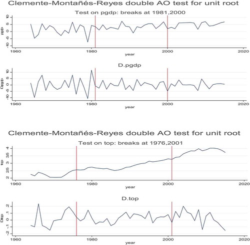
The result of two structural breakpoints in trade openness is positive and significant. This suggesting that any sudden shock has positive and permanent effects, and it is characterized by stationary around a mean, which changes in 1976 and 2001. Similarly, in the case of economic growth, there is evidence of one significant structural breakpoints, which varies in 1981. Moreover, empirical findings reveal the existence of single and double structural breaks in trade openness and economic growth variables. After finding the evidence of non-stationarity and structural breaks in variables, it is instructive to apply the cointegration between the variables of our interest. Therefore, the study has utilized the Engle and Granger (1987) and Enders and Siklos (2001) cointegration test to validate the long-run relationship between variables.

Figure 2. Clemente, Montanes, and Reyes (CMR) (1998) unit roots in the presence of a one-time structural break for economic growth (GDP) and trade openness (TOP) during the period 1960–2018.

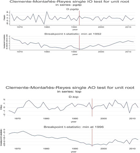
Figure 3. Clemente, Montanes, and Reyes (CMR) (1998) unit roots in the presence of a two-time structural break for economic growth (GDP) and trade openness (TOP) during the period 1960–2018.

4.2. Results of the threshold cointegration analysis

The threshold cointegration model is estimated using the consistent TAR (C-TAR) and consistent MTAR (C-MTAR) models. Table 4 reports the results of the Engle-Granger and threshold autoregressive cointegration models. Using TAR models in the full-sample period 1960–2018, and followed by the Chan (1993) method, results indicate that the estimated threshold values of C-TAR and C-MTAR are −1.421 and −3.422, respectively. The models support the Akaike Information Criterion (AIC) for the specific selection of lags. The AIC suggests the third lag for the C-TAR and C-MTAR models. Ljueng-Box (LB) test indicates the acceptance of the null hypothesis of no serial correlation and autocorrelation at least for order four and higher lags in all threshold models (TAR and MTAR). Moreover, the reported value of Ljueng-Box (LB) statistics suggests that the model is correctly specified and free from the autocorrelation.⁸ From the reported results in Table 4, it is evident that there is evidence of both linear and nonlinear cointegration between economic growth and trade openness in India. Figures 4 and 5 graphically present the threshold value of the TAR and M-TAR model.

Figure 4. The threshold value of the TAR model during the period 1960–2018.

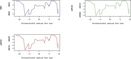
Figure 5. The threshold value of the M-TAR model during the period 1960–2018.

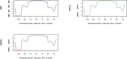
Table 4. Results of Engle-Granger and threshold cointegration tests during the period 1960–2018

Item	Engle-Granger	TAR	C-TAR	MTAR	C-MTAR
Lag		3	3	3	3
Threshold		0	−1.421	0	−3.422
${{\rho }_1}^{+}$†	2.557***	−2.162***	−2.155***	−2.171***	−2.176***
	[4.609]	[−5.883]	[−5.926]	[−5.785]	[−6.522]
${{\rho }_1}^{-}$		−1.969***	−1.964***	−1.982***	−1.802***
		[−5.84]	[−5.789]	[−5.945]	[−5.064]
Diagnostics Test
AIC	4.775	256.351	256.358	256.375	254.554
BIC		268.284	268.291	268.309	266.487
${\mathrm{Q}}_{\mathrm{L}\mathrm{B}}\left(4\right)$	_	0.994	0.992	0.996	0.998
${\mathrm{Q}}_{\mathrm{L}\mathrm{B}}\left(8\right)$	_	0.882	0.885	0.907	0.811
$Q_{LB}\left(12\right)$		0.698	0.715	0.748	0.739
Hypothesis Testing
${\mathrm{H}}_0$: No Symmetric Cointegration	0.210* (0.109)	19.838	19.832	19.818	21.338
${\mathrm{H}}_0$: No APT/cointegration	___	1.553	2.547*	1.531	2.230*
${\mathrm{H}}_0$: p-value		(0.261)	(0.101)	(0.270)	(0.102)
Total obs.	58	58	58	58	58
Cointegration obs.		54	54	54	54

Notes: † For the Engle-Granger cointegration test, ${\rho }_1$ refers to $\rho$ in Equation (6)(6) $\mathrm{\Delta }{\widehat{ϵ}}_{\mathrm{t}}={\rho }_1{\mathrm{I}}_{\mathrm{t}}{\widehat{ϵ}}_{\mathrm{t}-1}+{\rho }_2\left(1-{\mathrm{I}}_{\mathrm{t}}\right){\widehat{ϵ}}_{\mathrm{t}-1}+\sum _{\mathrm{i}=1}^{\mathrm{p}}{\mathrm{\varnothing }}_{\mathrm{i}}\mathrm{\Delta }{\widehat{ϵ}}_{\mathrm{t}-1}+{ϵ}_{\mathrm{t}}$(6) . For the Engle-Granger cointegration test, the critical values are −2.606, −1.946, and −1.613 at the 1%, 5%, and 10% level, respectively. AIC and BIC represent the Akaike information criterion and Bayesian information criterion. APT denotes asymmetric price transmission. ${\mathrm{Q}}_{\mathrm{L}\mathrm{B}}\left(\mathrm{p}\right)$ indicates the significance level for the Ljung-Box Q statistic; it tests serial correlation based on p autocorrelation coefficients (p = 4, 8, 12). $\varphi$ is the threshold cointegration test with the critical values from Enders and Siklos (2001). $F(H_0:{\rho }_1={\rho }_2)$ is a standard F-test to check the asymmetric price transmission between the variables of our interest. ***, **, * indicates significant at 1%, 5%, and 10% level, respectively. Numbers in brackets () and [] are p-values and t-statistics, respectively.

The C-TAR estimated threshold coefficient value is negative and significantly different zero, which suggests the evidence of threshold cointegration between economic growth and trade openness. Moreover, the threshold value $(\tau )$ and appropriate lag length selection are taken into consideration to examine the threshold cointegration between economic growth and trade openness in India. The diagnostic analysis has been checked by applying the AIC, BIC, and Ljung-Box Q statistics. AIC and BIC suggest the appropriate lags for correct model specifications. Besides, reported Ljueng-Box (LB) statistics indicate the absence of serial correlation for lag order up-to 12 in all specified models. Results said in Table 4 suggest that the $\mathrm{\Phi }$ test rejects the null hypothesis of no cointegration, $\mathrm{\Phi }(H_0:{\rho }_1={\rho }_2=0$) for C-TAR and C-MTAR models. The C-TAR model results suggest the evidence of threshold cointegration between economic growth and trade openness. Furthermore, results validate the cointegration with threshold error correction adjustment between economic growth and trade openness in India. After accepting the evidence of threshold cointegration between the variables, the study goes further to check whether the alignment towards the long-run equilibrium is asymmetric. Also, results reveal that the null hypothesis of symmetric adjustment $(H_0:{\rho }_1={\rho }_2)$ is rejected at the 10% level of significance for C-TAR and C-MTAR models. More specifically, the value of F-statistics for C-TAR and C-MTAR models is 2.547 and 2.230, and both statistics are statistically significant at the 10 percent level. Therefore, this suggests that the adjustment towards the long-run equilibrium is asymmetric, which further indicates that trade openness and economic growth respond differently to positive and negative deviations from their long-run equilibrium at a certain estimated threshold level.

Moreover, in both the models (C-TAR and C-MTAR), results report that $\left|{\rho }_1\right|>\left|{\rho }_2\right|$.⁹ This suggesting that the adjustment towards the long-run equilibrium tends to persist more for negative deviations and revert more quickly for positive deviations, which means the adjustment is faster while the economic growth is improving than the economic growth is worsening. Besides, results validate the presence of threshold cointegration and symmetric adjustments in both models. However, following the AIC and BIC criterion, we estimate the error correction mechanism for the C-MTAR model, which is considered to be more dynamic and advanced than the C-TAR model. Following the C-MTAR model, results reveal that economic growth and trade openness validate cointegration with asymmetric adjustment. Thus, this further suggests estimating the asymmetric error correction model (ACEM) for economic growth and trade openness variables in India. Eventually, to examine the causal relationship between economic growth and trade openness in the short and long-run, the research has used the AECM of Equations (12)(12) $\mathrm{\Delta }\mathrm{T}\mathrm{O}{\mathrm{P}}_{\mathrm{t}}={\theta }_{\mathrm{t}\mathrm{o}\mathrm{p}}+{\delta }_{\mathrm{t}\mathrm{o}\mathrm{p}}^{+}{\mathrm{E}}_{\mathrm{t}-1}^{+}+{\delta }_{\mathrm{t}\mathrm{o}\mathrm{p}}^{-}{\mathrm{E}}_{\mathrm{t}-1}^{-}+\sum _{\mathrm{j}=1}^{\mathrm{p}}{{\alpha }^{+}}_{\mathrm{t}\mathrm{o}\mathrm{p},\mathrm{j}}\mathrm{\Delta }{\mathrm{T}\mathrm{O}\mathrm{P}}_{\mathrm{t}-\mathrm{j}}^{+}+\sum _{\mathrm{j}=1}^{\mathrm{p}}{{\alpha }^{-}}_{\mathrm{t}\mathrm{o}\mathrm{p},\mathrm{j}}\mathrm{\Delta }{\mathrm{T}\mathrm{O}\mathrm{P}}_{\mathrm{t}-\mathrm{j}}^{-}+\sum _{\mathrm{j}=1}^{\mathrm{p}}{{\beta }^{+}}_{\mathrm{t}\mathrm{o}\mathrm{p},\mathrm{j}}\mathrm{\Delta }{\mathrm{G}\mathrm{D}\mathrm{P}}_{\mathrm{t}-\mathrm{j}}^{+}+\sum _{\mathrm{j}=1}^{\mathrm{p}}{{\beta }^{-}}_{\mathrm{t}\mathrm{o}\mathrm{p},\mathrm{j}}\mathrm{\Delta }{\mathrm{G}\mathrm{D}\mathrm{P}}_{\mathrm{t}-\mathrm{j}}^{-}+{\vartheta }_{\mathrm{t}\mathrm{o}\mathrm{p},\mathrm{t}}$(12) and (13(13) $\mathrm{\Delta }\mathrm{G}\mathrm{D}{\mathrm{P}}_{\mathrm{t}}={\theta }_{\mathrm{G}\mathrm{D}\mathrm{P}}+{\delta }_{\mathrm{G}\mathrm{D}\mathrm{P}}^{+}{\mathrm{E}}_{\mathrm{t}-1}^{+}+{\delta }_{\mathrm{G}\mathrm{D}\mathrm{P}}^{-}{\mathrm{E}}_{\mathrm{t}-1}^{-}+\sum _{\mathrm{j}=1}^{\mathrm{p}}{{\alpha }^{+}}_{\mathrm{G}\mathrm{D}\mathrm{P},\mathrm{j}}\mathrm{\Delta }{\mathrm{G}\mathrm{D}\mathrm{P}}_{\mathrm{t}-\mathrm{j}}^{+}+\sum _{\mathrm{j}=1}^{\mathrm{p}}{{\alpha }^{-}}_{\mathrm{G}\mathrm{D}\mathrm{P},\mathrm{j}}\mathrm{\Delta }{\mathrm{G}\mathrm{D}\mathrm{P}}_{\mathrm{t}-\mathrm{j}}^{-}+\sum _{\mathrm{j}=1}^{\mathrm{p}}{{\beta }^{+}}_{\mathrm{G}\mathrm{D}\mathrm{P},\mathrm{j}}\mathrm{\Delta }{\mathrm{T}\mathrm{O}\mathrm{P}}_{\mathrm{t}-\mathrm{j}}^{+}+\sum _{\mathrm{j}=1}^{\mathrm{p}}{{\beta }^{-}}_{\mathrm{G}\mathrm{D}\mathrm{P},\mathrm{j}}\mathrm{\Delta }{\mathrm{T}\mathrm{O}\mathrm{P}}_{\mathrm{t}-\mathrm{j}}^{-}+{\vartheta }_{\mathrm{G}\mathrm{D}\mathrm{P},\mathrm{t}}$(13) ) following the Chan (1993) procedure. The merit of applying the threshold cointegration with the AECM in this research is that it decomposes the original time series into four sub-series of the partial sum process of the positive and negative deviations. Besides, when we decompose the original series into two different series, then each having their both negative and positive deviations. Therefore, it becomes a four-time series to easily estimate the various parameters, which can explain their interrelationship between variables, .i.e., trade openness, and economic growth in India. For instance, Granger and Yoon (2002) have decomposed the series into the cumulative sum process of the positive and negative deviations to evaluate the non-linear cointegration and their adjustment between U.S. short-term and long-term interest rates, output and employment.¹⁰

4.3. Results of the asymmetric error-correction model (AECM)

We find that empirical results validate the long-run equilibrium relationship between economic growth and trade openness with asymmetric behaviour. Table 5 reports the estimated results of the AECM. Followed by the AIC, a maximum of up to eight lags has selected for estimation of the AECM. The diagnostic tests statistics (Q_LB) results reported in Table 5 indicate the absence of serial correlation in the model. Furthermore, ${\chi }^2($1.344) with a p-value of 0.102 suggests that economic growth Ganger causes trade openness in the short-run. In contrast, in the GDP equation, ${\chi }^2\left(0.401\right)$ with a p-value of 0.91 reveals the absence of Granger causality from trade openness to economic growth. In the next hypothesis, empirical results report that ${\chi }^2$ value is 0.129. However, it is not significantly different from zero. This suggesting that the null hypothesis of the absence of a distributed lag asymmetric effect from economic growth to trade openness is not rejected at the significance level. Similarly, the study does not find evidence of a significant cumulative asymmetric effect from trade openness to economic growth in India.

Table 5. Results of the asymmetric error correction model with threshold cointegration during the period 1960–2018

Parameters	GDP		TOP
	estimates	t-statistics	estimates	t-statistics
Θ	0.104*	1.973	−0.034	−0.026
α1^+	−0.011	−0.537	5.77	0.744
α2^+	−0.013	−0.764	−2.859	−0.393
α3^+	−0.002	−0.147	1.131	0.158
α4^+	−0.005	−0.757	2.112	0.298
α1^‒	−0.019	−0.815	−8.325	−0.779
α2^‒	−0.003	−0.164	−8.324	−0.765
α3^‒	−0.006	−0.44	−9.906	−0.93
α4^‒	0.004	0.393	−1.732	−0.145
β1^+	−0.096	−0.301	1.03**	2.056
β2^+	0.134	0.451	0.697*	1.676
β3^+	−0.375	−1.276	0.224	0.728
β4^+	−0.059	−0.205	0.014	0.086
β1^‒	0.776*	1.774	0.912.	1.585
β2^‒	−0.09	−0.202	0.733*	1.704
β3^‒	0.41	0.941	0.778**	2.416
β4^‒	0.266	0.544	0.123	0.451
δ ^+	0.015	0.632	−2.336***	−4.01
δ ^‒	0.022	0.759	−1.958***	−2.731
R^2	0.236	_	0.746	_
AIC	−79.107	_	259.581	_
BIC	−39.701	_	298.987	_
Q LB (4)	0.931	_	0.476	_
Q LB (8)	0.990	_	0.371	_
H01: α1^+ = α1^‒ = 0 for all lags	0.765	[0.64]	0.651	[0.73]
H02: βi^+ = βi^‒ = 0 for all lags	0.401	[0.91]	1.344*	[0.102]
H03: α2^+ = α2^‒	0.129	[0.72]	0.129	[0.71]
H04: β4^+ = β4^‒	0.568	[0.46]	0.123	[0.73]
H05: $\sum _{i=1}^4{\alpha }_i+=\sum _{i=1}^4{\alpha }_i-$	2.148	[0.15]	1.383	[0.25]
H06: $\sum _{i=1}^4{\beta }_i+=\sum _{i=1}^4{\beta }_i-$	0.127	[0.72]	1.263	[0.27]
H07: δ ^+ = δ ^‒	0.115	[0.74]	0.532	[0.47]

Numbers in brackets [] are p-values. The hypotheses, H_01, and H₀₂, evaluate the Granger causality tests, H₀₃and H₀₄ evaluate distributed asymmetric lag effect, H₀₅ and H₀₆ assess the cumulative asymmetric effect and H₀₇ evaluates the equilibrium adjustment path asymmetric effect.

***, **, * indicates significant at the 1%, 5%, 10% level, respectively.

Empirical results reveal that the equilibrium adjustment path asymmetric effect $(H_{07}:{\delta }^{+}={\delta }^{-})$ ${\chi }^2$ values are 0.115, and 0.532, respectively, and these statistics are not significantly different from zero. Thus, this suggests that there is an absence of equilibrium adjustment path asymmetric effect between economic growth and trade openness. Furthermore, the coefficients of error correction terms in model (12) are significantly different from zero in case of negative and positive deviations. This suggesting that economic growth responds to disequilibrium in the economy when the trade share in GDP is deteriorating or improving. Furthermore, empirical findings exhibit that when trade share in GDP is worsening, then restoring the equilibrium could be possible by adjusting the increasing economic growth in India.

4.4. Robustness checks

To assess the robustness of the results, and to evaluate the impact of trade reforms on economic growth in India, we have relatively shortened our time series data into two sub-samples. In Section 4.1, we have already corroborated the presence of structural breaks in economic growth and trade openness during the period of the 1990 s. India took the initiative of massive reforms of its external sector by adopting the series of steps in trade reforms during the 1990 s to boost export competitiveness and improve the situation of the BOP crisis. In sum, considering the relevance of structural breaks and evaluating the trade reforms’ impact on economic growth, we split the full-sample data into two sub-samples, deemed to be pre-reforms period, i.e., 1960–1990, and post reforms period, i.e., 1991–2018. Table 6 reports the results of the pre-reforms period. Re-estimated results during the pre-reforms period, have passed all diagnostics tests like serial correlation and endogeneity by including the lag effect of the regressors (see Table 6).

Table 6. Results of Engle-Granger and threshold cointegration tests during the pre-reforms period 1960–1990

Item	Engle-Granger	TAR	C-TAR	MTAR	C-MTAR
Lag		3	3	3	3
Threshold		0	−2.979	0	−3.431
${{\rho }_1}^{+}$†	−1.459***	−2.329***	−2.331***	−2.428***	−2.352***
	[−4.937]	[−4.116]	[−4.509]	[−4.27]	[−4.702]
${{\rho }_1}^{-}$		−2.004***	−1.847***	−1.994***	−1.779***
		[−3.95]	[−3.555]	[−4.009]	[−3.474]
Diagnostics Test
AIC	5.	138.547	137.355	137.852	136.275
BIC		146.095	144.903	145.4	143.824
${\mathrm{Q}}_{\mathrm{L}\mathrm{B}}\left(4\right)$	_	0.989	0.956	0.994	0.995
${\mathrm{Q}}_{\mathrm{L}\mathrm{B}}\left(8\right)$	_	0.978	0.925	0.954	0.868
$Q_{LB}\left(12\right)$		0.744	0.763	0.841	0.899
Hypothesis Testing
${\mathrm{H}}_0$: No Symmetric Cointegration	0.223 [1.167]	9.268	10.195	9.803	11.072
${\mathrm{H}}_0$: No APT/Cointegration		0.746	1.766	1.336	2.732*
${\mathrm{H}}_0$: p-value		(0.397)	(0.198)	(0.261)	(0.103)
Total obs.		30	30	30	30
Cointegration obs.		26	26	26	26

Notes: † For the Engle-Granger cointegration test, ${\rho }_1$ refers to $\rho$ in Equation (6)(6) $\mathrm{\Delta }{\widehat{ϵ}}_{\mathrm{t}}={\rho }_1{\mathrm{I}}_{\mathrm{t}}{\widehat{ϵ}}_{\mathrm{t}-1}+{\rho }_2\left(1-{\mathrm{I}}_{\mathrm{t}}\right){\widehat{ϵ}}_{\mathrm{t}-1}+\sum _{\mathrm{i}=1}^{\mathrm{p}}{\mathrm{\varnothing }}_{\mathrm{i}}\mathrm{\Delta }{\widehat{ϵ}}_{\mathrm{t}-1}+{ϵ}_{\mathrm{t}}$(6) . For the Engle-Granger cointegration test, the critical values are −2.62, −1.95, and −1.61 at the 1%, 5%, and 10% level, respectively. AIC and BIC represent the Akaike information criterion and Bayesian information criterion. APT denotes asymmetric price transmission. ${\mathrm{Q}}_{\mathrm{L}\mathrm{B}}\left(\mathrm{p}\right)$ indicates the significance level for the Ljung-Box Q statistic; it tests serial correlation based on p autocorrelation coefficients (p = 4, 8, 12). $\varphi$ is the threshold cointegration test with the critical values from Enders and Siklos (2001). $F(H_0:{\rho }_1={\rho }_2)$ is a standard F-test to check the asymmetric price transmission between the variables of our interest. ***, **, * indicates significant at the 1%, 5%, and 10% level. Numbers in brackets () and [] are p-values and t-statistics, respectively.

The results reported in Table 6 seem to be similar and consistent with the results described in Table 4. Specifically, during the pre-reforms period, we find evidence of threshold cointegration between economic growth and trade openness in India. Moreover, the null hypothesis of symmetric adjustment (linear adjustment) is rejected at a 10% level for the C-MTAR model. Therefore, this suggests that adjustment towards the long-run equilibrium is asymmetric. Furthermore, this also suggests that trade openness and economic growth respond differently to positive and negative deviations. Similarly, post reforms sub-samples period 1991–2018, threshold cointegration results are reported in Table 7. It is important to note here that our post-reforms sub-period estimated the threshold model indicates the evidence of linear cointegration and linear adjustment between economic growth and trade openness in India. We do not find any significant evidence of asymmetric adjustment between the variables after the trade reforms in India. However, in the first re-estimated models (1960–1990) and both TAR and MTAR models, $\left|{\rho }_1\right|>\left|{\rho }_2\right|$. Therefore, this suggests that the speed of adjustment is faster, in positive deviations than the negative deviations. More specifically, results exhibits that economic growth is quickly adjusted and reverts to equilibrium while trade share is improving than the period while the trade share is deteriorating.

Table 7. Results of Engle-Granger and threshold cointegration tests during the post-reforms period 1991–2018

Item	Engle-Granger	TAR	C-TAR	MTAR	C-MTAR
Lag		3	3	3	3
Threshold		0	−2.048	0	0.602
${{\rho }_1}^{+}$†	−1.112***	−1.377**	−1.282**	−1.246**	−1.043
	[−4.175]	[−2.459]	[−2.286]	[−2.138]	[−1.573]
${{\rho }_1}^{-}$		−1.515**	−1.6***	−1.562***	−1.489***
		[−2.753]	[−2.91]	[−2.953]	[−2.975]
Diagnostics Test
AIC		103.727	103.269	103.25	102.783
BIC		110.795	110.338	110.318	109.851
${\mathrm{Q}}_{\mathrm{L}\mathrm{B}}\left(4\right)$	_	0.997	0.999	0.998	0.99
${\mathrm{Q}}_{\mathrm{L}\mathrm{B}}\left(8\right)$	_	0.976	0.962	0.887	0.822
$Q_{LB}\left(12\right)$		0.673	0.708	0.543	0.472
Hypothesis Testing
${\mathrm{H}}_0$: No Symmetric Cointegration	0.166 [0.912]	4.11	4.372	4.383	4.656
${\mathrm{H}}_0$: No APT/Cointegration		0.097	0.465	0.481	0.863
${\mathrm{H}}_0$: p-value		(0.759)	(0.504)	(0.496)	(0.364)
Total obs.		28	28	28	28
Cointegration obs.		24	24	24	24

Notes: † For the Engle-Granger cointegration test, ${\rho }_1$ refers to $\rho$ in Equation (6)(6) $\mathrm{\Delta }{\widehat{ϵ}}_{\mathrm{t}}={\rho }_1{\mathrm{I}}_{\mathrm{t}}{\widehat{ϵ}}_{\mathrm{t}-1}+{\rho }_2\left(1-{\mathrm{I}}_{\mathrm{t}}\right){\widehat{ϵ}}_{\mathrm{t}-1}+\sum _{\mathrm{i}=1}^{\mathrm{p}}{\mathrm{\varnothing }}_{\mathrm{i}}\mathrm{\Delta }{\widehat{ϵ}}_{\mathrm{t}-1}+{ϵ}_{\mathrm{t}}$(6) . For the Engle-Granger cointegration test, the critical value is −2.62, −1.95, and −1.61 at the 1%, 5%, and 10% level, respectively. AIC and BIC represent the Akaike information criterion and Bayesian information criterion. APT denotes asymmetric price transmission. ${\mathrm{Q}}_{\mathrm{L}\mathrm{B}}\left(\mathrm{p}\right)$ indicates the significance level for the Ljung-Box Q statistic; it tests serial correlation based on p autocorrelation coefficients (p = 4, 8, 12). $\varphi$ is the threshold cointegration test with the critical values from Enders and Siklos (2001). $F(H_0:{\rho }_1={\rho }_2)$ is a standard F-test to check the asymmetric price transmission between the variables of our interest. ***, **, * indicates significant at the 1%, 5%, and 10% level. Numbers in brackets () and [] are p-values and t-statistics, respectively.

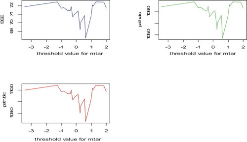
Nevertheless, during the post-reforms period, we find substantial evidence that negative deviation exceeds the positive deviation ($\left|{\rho }_1\right|<\left|{\rho }_2\right|$). This suggesting that the speed of adjustment is quite faster during the trade openness deteriorating situation than the trade openness improving situation. Thus, this further indicates that economic growth reverts to an equilibrium position quickly when there is a situation of trade openness decreases. This result is not surprising as India has faced a severe imbalance in growth in the trade after the post-reforms period. One plausible to note that India has a large consumer market economy, and the demand for crude oil has been persistently increasing since after the trade reforms for its industrial expansion and to maintain sustainable and high economic growth. This persistent rise in crude oil prices has aggravated the trade balance and widening trade deficit in India. Therefore, empirical results suggest that economic growth could revert quickly to equilibrium condition when the degree of trade openness is deteriorating. Figures 6–9 depict the graphical presentation of the threshold value of the TAR and M-TAR models during the pre-and post-trade reforms periods in India.

Figure 6. The threshold value of the TAR model during the pre-reforms period 1960–1990.

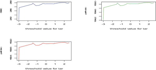
Figure 7. The threshold value of the M-TAR model during the pre-reforms period 1960–1990.

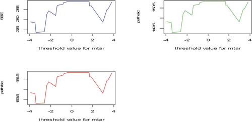
Figure 8. The threshold value of the TAR model during the post-reforms period 1991–2018.

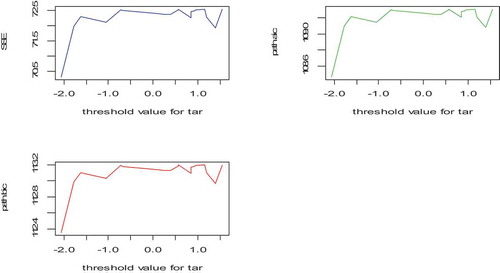
Figure 9. The threshold value of the M-TAR model during the post-reforms period 1991–2018.

After finding the evidence of cointegration with asymmetric adjustment during the pre-and post-trade reforms period in India, we set up an AECM over the different sub-periods. Tables 8 and 9 report the re-estimated AECM results of the pre-and post-trade reforms periods. Using the F-test, we test the Granger causality between economic growth and trade openness in India over the pre-reforms and post-trade reforms period. In the trade openness equations, we reject the null of $H_{02}:{\beta }_i^{+}={\beta }_i^{-}=0$ for all lags (see Table 8). This suggesting that economic growth Ganger causes trade openness, whereas the reverse is not valid. Similarly, we test other hypotheses to evaluate the distributed lag asymmetric effect, cumulative asymmetric effect, and equilibrium adjustment path asymmetric effects between variables while the lags vary from 1 to 4. Empirical results exhibit evidence of distributed lag asymmetric effect for its own lagged values of trade openness. Thus, this suggests that the previous year’s positive and negative deviations in trade-openness have an asymmetrical impact on the current year trade openness. The F-statistics of 0.346 and 1.932 to test the null of H₀₅:$\sum _{\mathrm{i}=1}^4{\alpha }_{\mathrm{i}}+=\sum _{\mathrm{i}=1}^4{\alpha }_{\mathrm{i}}-$ is not statistically significant. Thus, this reveals that cumulative asymmetric effects for its own lagged values are symmetric. However, as we reject the null of H₀₆: $\sum _{\mathrm{i}=1}^4{\beta }_{\mathrm{i}}+=\sum _{\mathrm{i}=1}^4{\beta }_{\mathrm{i}}-$, so there is evidence of the cumulative asymmetric impact of trade openness on economic growth in India and vice versa.

Table 8. Results of the asymmetric error correction model with threshold cointegration during the pre-reforms period 1960–1990

Parameters	GDP		TOP
	Estimates	t-statistics	estimates	t-statistics
Θ	0.136*	1.263	3.58	1.333
α1^+	0.398	0.667	−21.396	−1.466
α2^+	−0.609*	−1.791	19.417	1.031
α3^+	0.304	0.4	−33.08.	−1.776
α4^+	0.24	0.33	28.737	1.614
α1^‒	−0.087	−0.105	14.252	0.704
α2^‒	0.434	0.486	−45.958*	−2.105
α3^‒	0.69	0.792	−5.571	−0.261
α4^‒	0.373	0.402	−31.301	−1.377
β1^+	−0.005	−0.105	1.787	1.563
β2^+	−0.038	−0.922	2.444**	2.451
β3^+	−0.012	−0.345	0.059	0.072
β4^+	−0.003	−0.236	−0.342	−1.111
β1^‒	−0.028	−0.535	3.559**	2.759
β2^‒	0.01	0.261	1.429	1.507
β3^‒	−0.016	−0.567	2.215**	3.203
β4^‒	0.009	0.357	0.187	0.314
δ ^+	0.008	0.155	−3.533**	−2.849
δ ^‒	0.026	0.414	−4.964**	−3.258
R^2	0.652	_	0.926	_
AIC	−34.232	_	125.646	_
BIC	−9.854	_	150.024	_
Q LB (4)	0.722	_	0.966	_
Q LB (8)	0.96	_	0.271	_
H01: α1^+ = α1^‒ = 0 for all lags	0.516	[0.81]	1.415	[0.35]
H02: βi^+ = βi^‒ = 0 for all lags	0.597	[0.76]	2.066***	[0.02]
H03: α2^+ = α2^‒	0.614	[0.46]	4.033*	[0.09]
H04: β4^+ = β4^‒	0.27	[0.62]	0.925	[0.37]
H05: $\sum _{\mathrm{i}=1}^4{\alpha }_{\mathrm{i}}+=\sum _{\mathrm{i}=1}^4{\alpha }_{\mathrm{i}}-$	0.346	[0.58]	1.932	[0.21]
H06: $\sum _{\mathrm{i}=1}^4{\beta }_{\mathrm{i}}+=\sum _{\mathrm{i}=1}^4{\beta }_{\mathrm{i}}-$	0.299**	[0.06]	5.92*	[0.05]
H07: δ ^+ = δ ^‒	0.206	[0.67]	2.205	[0.19]

Notes: Numbers in brackets [] are p-values. The hypotheses, H_01, and H₀₂ evaluate the Granger causality tests, H₀₃ and H₀₄ evaluate distributed asymmetric lag effect, H₀₅ and H₀₆ assess the cumulative asymmetric effect and H₀₇ evaluates the equilibrium adjustment path asymmetric effect. ***, **, * indicates significant at the 1%, 5%, 10% level, respectively.

Table 9. Results of the asymmetric error correction model with threshold cointegration during the post-reforms period 1991–2018

Parameters	GDP		TOP
	estimates	t-statistics	estimates	t-statistics
Θ	0.092	0.3	1.425	0.346
α1^+	−0.421	−0.242	27.889*	1.692
α2^+	1.101	0.716	−9.265	−0.448
α3^+	0.275	0.233	−19.75	−1.245
α4^+	−0.657	−0.561	−7.735	−0.491
α1^‒	1.437*	1.807	−7.009	−0.292
α2^‒	0.001	0.001	−9.644	−0.717
α3^‒	−1.513	−0.77	13.072	0.494
α4^‒	1.341	0.44	1.524	0.037
β1^+	−0.023	−0.203	0.956	0.639
β2^+	0.018	0.155	−0.82	−0.515
β3^+	−0.024	−0.418	−0.295	−0.376
β4^+	−0.029*	−1.792	0.374	0.749
β1^‒	0.025	0.21	0.075	0.046
β2^‒	−0.029	−0.281	0.495	0.359
β3^‒	0.003	0.04	0.204	0.19
β4^‒	0.006	0.075	−0.048	−0.048
δ ^+	−0.026*	1.198	−1.995*	−1.167
δ ^‒	−0.012	−0.076	−0.724	−0.328
R^2	0.661	_	0.901	_
AIC	−29.319	_	90.289	_
BIC	−6.609	_	112.999	_
Q LB (4)	0.593	_	0.391	_
Q LB (8)	0.923	_	0.427	_
H01: α1^+ = α1^‒ = 0 for all lags	0.426	[0.86]	1.691*	[0.103]
H02: βi^+ = βi^‒ = 0 for all lags	0.271	[0.94]	1.634*	[0.094]
H03: α2^+ = α2^‒	0.405	[0.56]	0	[0.99]
H04: β4^+ = β4^‒	0.224	[0.66]	0.18	[0.69]
H05: $\sum _{\mathrm{i}=1}^4{\alpha }_{\mathrm{i}}$^+ = $\sum _{\mathrm{i}=1}^4{\alpha }_{\mathrm{i}}$^‒	0.029	[0.87]	0.008	[0.93]
H06: $\sum _{\mathrm{i}=1}^4{\beta }_{\mathrm{i}}$^+ = $\sum _{\mathrm{i}=1}^4{\beta }_{\mathrm{i}}$^‒	0.103	[0.76]	0.037	[0.86]
H07: δ ^+ = δ ^‒	0.155	[0.71]	0.95	[0.38]

Notes: Numbers in brackets [] are p-values. The hypotheses, H_01, and H₀₂ evaluate the Granger causality tests, H₀₃andH₀₄ evaluate distributed asymmetric lag effect, H₀₅ and H₀₆ assess the cumulative asymmetric effect and H₀₇ evaluates the equilibrium adjustment path asymmetric effect. ***, **, * indicates significant at 1%, 5%, 10% level, respectively.

On the other hand, during the post-reforms period, we find evidence that economic growth Granger causes trade openness, whereas the reverse is not true (see Table 9).¹¹ This empirical inference is consistent with the pre-reforms period results. Furthermore, we do not find any empirical evidence of distributed lag asymmetric, cumulative asymmetric, and the equilibrium adjustment path asymmetric effects between the two series during the post reforms period. Thus, this indicates that cumulative and equilibrium adjustment path effects are symmetrical. Notwithstanding, we find evidence that the cumulative effects are asymmetrical between economic growth and trade openness during the pre-reforms period. Finally, we evaluate the momentum equilibrium adjustment asymmetry during the pre-and post-reforms period. The estimated ${\delta }^{+}$ and ${\delta }^{-}$ coefficients are −3.533 and −4.964, respectively. Also, both estimated coefficients are statistically significant at the 1% level. The magnitude of both factors is negative, so the sign is correct. In sum, this indicates that in the short-run trade openness response to positive and negative deviations by 353.3% and 496.4%, respectively. Therefore, the positive and negative divergences are disappeared entirely within one month approximately and less than a month (around 20 days), respectively. Similarly, during the post-reforms period and in the short-run, the positive deviations in trade openness entirely disappear approximately before the two months. Notwithstanding, economic growth response to positive deviations in trade openness is substantially slow, such that it takes about 38 months to digest and revert to long-run equilibrium fully.¹² In sum, during the pre-reforms period, results exhibit the slower responsiveness of trade share in GDP to positive deviations from the long-run equilibrium relationship than negative deviations.

5. Conclusions

This study aims at revealing the adjustment process of the economic growth in response to changes in trade openness. We provide new evidence that the economic growth responds asymmetrically to changes in trade openness in India during the period 1960–2018 and during the pre-trade reforms period 1960–1990 and post-trade reforms period 1991–2018. The results reveal that the long-run dynamics between economic growth and trade openness exhibit asymmetry. Furthermore, this study shows a uni-directional causal relationship between economic growth and trade openness in India. Specifically, the research exhibits that economic growth Granger causes trade openness during the full-sample period and over the sub-samples of the pre-and post-trade reforms period. Based on our findings from the asymmetric error-correction analysis, we conclude that positive deviations in trade share in GDP (trade openness) are highly responsive such that it quickly reverts to equilibrium than the negative deviations during the period 1960–2018. Notwithstanding, during the pre-trade reforms period, trade openness response to positive and negative deviations are fully removed within approximately one month and less than a month, respectively. Moreover, in the short-run and during the pre-reforms period, the error-correction model reveals that disturbances in trade openness fully digest positive and negative economic growth shocks within a month and less than a month, respectively. However, despite this high speed of adjustment in trade share in GDP, we are unable to reject the evidence of equilibrium adjustment path asymmetric effect during the period under study and over the sub-periods. From a different perspective, this could indicate that the adjustment path of economic growth in response to changes in trade openness might be nonlinear.

There is a possibility that apart from the economic growth and trade openness, there could be several other independent variables like exchange rate, foreign direct investment (FDI) can affect the transmission between economic growth and trade openness in India. However, despite this shortcoming, the study has only considered the bivariate framework model, such that it examines the one-to-one reaction upon each other. In future research, we would like to explore the linear vs. nonlinear cointegration, and their asymmetric adjustment incorporating the multivariate independent variables. Moreover, we would also like to examine the trade openness impact on the economic growth of developing countries. Therefore, in the future, it could be worthwhile to investigate the panel threshold model for the asymmetric transmission between economic growth and trade openness, including certain other macroeconomic factors, which could substantially help in diffusing the technology from advanced economies to developing economies. Finally, we find the relevance of trade share in GDP in India. Therefore, the study suggests that policymakers can give priority to import substitution, export promotion, and trade liberalization policies, such that the degree of trade openness can substantially raise the economic growth in India. Furthermore, it could be recommended by the policymakers that the combination of import substitution vs. export promotion and trade liberalization facilitates economic growth both directly and indirectly in India.

Acknowledgements

We would like to thank Juan Sapena, Editor of the journal, for giving us a chance to revise this paper. We are thankful to both anonymous referees for their valuable comments and insightful suggestions, which enabled us to improve the quality of this paper to a large extent.

Additional information

Funding

The authors received no direct funding for this research.

Notes on contributors

Lingaraj Mallick

Lingaraj Mallick is working as an Assistant Professor of Economics, School of Social Sciences, Maulana Azad National Urdu University, Hyderabad, India. He is researching an exchange rate and trade balance in emerging countries, and time series econometrics. He teaches macroeconomics, mathematical economics, and econometrics. Lingaraj Mallick can be contacted at [email protected]

Smruti Ranjan Behera

Smruti Ranjan Behera is working as an Associate Professor of Economics in the Department of Humanities and Social Sciences, Indian Institute of Technology Ropar, Punjab, India. He teaches econometrics, macroeconomics, international economics, urban economics, and applied econometrics. His research interest includes FDI and innovation, FDI and technology spillover in the Indian manufacturing industries, purchasing power parity, current account, and saving-investment dynamics and international capital mobility to the developing countries. Smruti Ranjan Behera can be contacted at [email protected]

Notes

1. For an extensive survey of literature related to the trade openness and economic growth, see Yanikkaya (2003).

2. The detailed discussion of the construction of the economic growth variable has been discussed in Section 3.

3. TAR represents the threshold autoregressive, and MTAR represents the momentum threshold autoregressive.

4. Note that existing studies have taken GDP per capita to measure the economic growth of countries (Al-Shayeb & Hatemi-J, 2016; Yanikkaya, 2003; Zahonogo, 2016). To measure the economic growth of a country, previous studies (Gries et al., 2009) also use the logarithm of real GDP per capita (log-level data). Furthermore, for notational simplifications, we have used the abbreviation term, such as GDP, in place of economic growth.

5. DU indicates intercept dummy for a change in the level ($D{U}_t=1ift>TB)$; TB represents a change in the slope of the trend function, or we can say the periods where the mean is modified.

6. More recently, Mallick et al. (2020) have discussed different kinds of hypotheses to evaluate the asymmetric cointegration between WPI and CPI in India. Also, they have used the bivariate analysis to assess the asymmetric cointegration between variables.

7. Note that to conserve the space, we have not reported the one-time structural breaks statistics. However, we have reported the graphical presentation of both one and two-time structural breaks in Figures 2 and 3. One-time structural breaks results could be available from the authors upon request.

8. This research has studied the threshold cointegration between economic growth and trade openness in India. The threshold cointegration with AECM inevitably checks the serial correlation by including the specific lag of the regressors (Enders & Siklos, 2001). Also, the threshold cointegration corrects the autocorrelation and endogeneity in the models. AECM with threshold regression consists of the lag effect of the regressors up-to-the significance level, followed by AIC/BIC. Therefore, the additional parameters automatically generated in these models solve the problem of small sample size bias, and the estimated parameters could be adjusted to less biased. Besides, followed by previous studies (e.g., Dedeoglu & Ogut, 2017; Jibrilla Aliyu & Mohammed, 2015), this study has applied threshold cointegration between economic growth and trade openness with small size time-series data. Also, specific to our bivariate analysis in this study, the non-linear models generate parameters to measure the positive and negative speed of reaction and their adjustments. Therefore, AECM gives better ideas of the positive and negative speed of adjustment while reverting to the long-run equilibrium following temporary shock in the short-run. Also, AECM provides a clear picture of non-linear adjustment of positive and negative shocks and their rate of reaction during the different regimes, i.e., degree of adaptation below and above the estimated threshold value.

9. Note that ${\rho }_1$ and ${\rho }_2$ refers to the positive and negative deviations in the threshold autoregressive model.

10. This research has used Enders and Siklos (2001) non-linear approach to evaluate the threshold cointegration and asymmetric adjustment between trade openness and economic growth in India. Therefore, followed by Enders and Siklos (2001), Granger and Yoon (2002), and Frey and Manera (2007), we have decomposed the original series in our study into four sub-series of the partial sum process of the positive and negative deviations. Therefore, in the AECM sixteen $\alpha$ and $\beta$ parameters are estimated including the positive and negative speed of adjustment parameters (${\delta }^{+},{\delta }^{-}$) and constant parameter ($\theta ).$ Moreover, the $\alpha$ and $\beta$ parameters represent the cumulative sum of positive and negative deviations, which measures the interrelationship between trade openness and economic growth. Tables 5, 8, and 9 reports the results of AECM during the full-sample period, and over different sub-periods of the study.

11. The F-statistics of 1.634 is statistically significant at the 10% level. Therefore, we reject the null of H₀₂: β_i⁺ = β_i^‒ = 0 for all lags in the trade-openness equation, which indicates the presence of Granger causality from economic growth to trade openness in India during the post-reforms period.

12. $\frac{1}{3.533}=0.283\approx onemonth,\frac{1}{4.964}=0.201\approx 20days,$ $\frac{1}{1.995}=0.501\approx 50days,\frac{1}{0.026}=38.46months$ $\approx 3years.$

References

- Agrawal, P. (2015). The role of exports in India’s economic growth. The Journal of International Trade & Economic Development, 24(6), 835–26. https://doi.org/10.1080/09638199.2014.968192
- Almeida, R., & Fernandes, A. M. (2008). Openness and technological innovations in developing countries: Evidence from firm-level surveys. The Journal of Development Studies, 44(5), 701–727. https://doi.org/10.1080/00220380802009217
- Al-Shayeb, A., & Hatemi-J, A. (2016). Trade openness and economic development in the UAE: An asymmetric approach. Journal of Economic Studies, 43(4), 587–597. https://doi.org/10.1108/JES-06-2015-0094
- Anderson, J. E., & Neary, J. P. (1992). Trade reform with quotas, partial rent retention, and tariffs. Econometrica, 60(1), 57–76. https://doi.org/10.2307/2951676
- Bahmani-Oskooee, M., & Niroomand, F. (1999). Openness and economic growth: An empirical investigation. Applied Economics Letters, 6(9), 557–561. https://doi.org/10.1080/135048599352592
- Balke, N. S., & Fomby, T. B. (1997). Threshold cointegration. International Economic Review, 38(3), 627–645. https://doi.org/10.2307/2527284
- Birinci, S. (2013). Trade openness, growth, and informality: Panel VAR evidence from OECD economies. Economics Bulletin, 33(1), 694–705. http://www.accessecon.com/Pubs/EB/2013/Volume33/EB-13-V33-I1-P66.pdf
- Bond, E. W., Jones, R. W., & Wang, P. (2005). Economic takeoffs in a dynamic process of globalization. Review of International Economics, 13(1), 1–19. https://doi.org/10.1111/j.1467-9396.2005.00489.x
- Chan, K. S. (1993). Consistency and limiting distribution of the least squares estimator of a threshold autoregressive model. The Annals of Statistics, 21(1), 520–533. https://doi.org/10.1214/aos/1176349040
- Chandra, R. (2003). Reinvestigating export-led growth in India using a multivariate cointegration framework. The Journal of Developing Areas, 37(1), 73–86. https://doi.org/10.1353/jda.2004.0005
- Chang, R., Kaltani, L., & Loayza, N. V. (2009). Openness can be good for growth: The role of policy complementarities. Journal of Development Economics, 90(1), 33–49. https://doi.org/10.1016/j.jdeveco.2008.06.011
- Clemente, J., Montanes, A., & Reyes, M. (1998). Testing for a unit root in variables with a double change in the mean. Economics Letters, 59(2), 175–182. https://doi.org/10.1016/S0165-1765(98)00052-4
- Das, A., & Paul, B. P. (2011). Openness and growth in emerging Asian economies: Evidence from GMM estimations of a dynamic panel. Economics Bulletin, 31(3), 2219–2228. http://www.accessecon.com/Pubs/EB/2011/Volume31/EB-11-V31-I3-P201.pdf
- Dedeoglu, D., & Ogut, K. (2017). Asymmetric cointegration with threshold adjustment model of exchange rates and the trade balance in Turkey. The Journal of International Trade & Economic Development, 26(2), 174–194. https://doi.org/10.1080/09638199.2016.1233288
- Dollar, D. (1992). Outward-oriented developing economies really do grow more rapidly: Evidence from 95 LDCs, 1976–1985. Economic Development and Cultural Change, 40(3), 523–544. https://doi.org/10.1086/451959
- Dollar, D., & Kraay, A. (2004). Trade, growth, and poverty. The Economic Journal, 114(493), F22–F49. https://doi.org/10.1111/j.0013-0133.2004.00186.x
- Edwards, S. (1993). Openness, trade liberalization, and growth in developing countries. Journal of Economic Literature, 31(3), 1358–1393. https://www.jstor.org/stable/2728244
- Enders, W., & Granger, C. W. J. (1998). Unit-Root tests and asymmetric adjustment with an example using the term structure of interest rates. Journal of Business & Economic Statistics, 16(3), 304–311. https://www.jstor.org/stable/1392506
- Enders, W., & Siklos, P. L. (2001). Cointegration and Threshold Adjustment. Journal of Business & Economic Statistics, 19(2), 166–176. https://doi.org/10.1198/073500101316970395
- Engle, R. F., & Granger, C. W. (1987). Co-integration and error correction: Representation, estimation, and testing. Econometrica, 55(2), 251–276. https://doi.org/10.2307/1913236
- Eriṣ, M. N., & Ulaṣan, B. (2013). Trade openness and economic growth: Bayesian model averaging estimate of cross-country growth regressions. Economic Modelling, 33(C), 867–883. https://doi.org/10.1016/j.econmod.2013.05.014
- Frankel, J. A., & Romer, D. H. (1999). Does trade cause growth? American Economic Review, 89(3), 379–399. https://doi.org/10.1257/aer.89.3.379
- Freund, C., & Bolaky, B. (2008). Trade, regulations, and income. Journal of Development Economics, 87(2), 309–321. https://doi.org/10.1016/j.jdeveco.2007.11.003
- Frey, G., & Manera, M. (2007). Econometric models of asymmetric price transmission. Journal of Economic Surveys, 21(2), 349–415. https://doi.org/10.1111/j.1467-6419.2007.00507.x
- Goldberg, P., Khandelwal, A., Pavcnik, N., & Topalova, P. (2010). Imported intermediate inputs and domestic product growth: Evidence from India. The Quarterly Journal of Economics, 125(4), 1727–1767. https://doi.org/10.1162/qjec.2010.125.4.1727
- Granger, C. W., & Yoon, G. (2002). Hidden cointegration. U of California, Economics Working Paper, ( 2002–02). https://doi.org/10.2139/ssrn.313831
- Gries, T., Kraft, M., & Meierrieks, D. (2009). Linkages between financial deepening, trade openness, and economic development: Causality evidence from Sub-Saharan Africa. World Development, 37(12), 1849–1860. https://doi.org/10.1016/j.worlddev.2009.05.008
- Grossman, G. M., & Helpman, E. (1991). Trade, knowledge spillovers, and growth. European Economic Review, 35(2–3), 517–526. https://doi.org/10.1016/0014-2921(91)90153-A
- Hamdi, H., & Sbia, R. (2013). The relationship between natural resources rents, trade openness, and economic growth in Algeria. Economics Bulletin, 33(2), 1649–1659. http://www.accessecon.com/Pubs/EB/2013/Volume33/EB-13-V33-I2-P154.pdf
- Harrison, A. (1996). Openness and growth: A time-series, cross-country analysis for developing countries. Journal of Development Economics, 48(2), 419–447. https://doi.org/10.1016/0304-3878(95)00042-9
- Hye, Q., Lau, W.-Y., & Tourres, M.-A. (2014). Does economic liberalization promote economic growth in Pakistan? An empirical analysis. Quality & Quantity, 48(4), 2097–2119. https://doi.org/10.1007/s11135-013-9882-9
- Hye, Q. M. A., & Lau, W.-Y. (2014). Trade openness and economic growth: Empirical evidence from India. Journal of Business Economics and Management, 16(1), 188–205. https://doi.org/10.3846/16111699.2012.720587
- Irwin, D. A., & Terviö, M. (2002). Does trade raise income? Evidence from the twentieth century. Journal of International Economics, 58(1), 1–18. https://doi.org/10.1016/S0022-1996(01)00164-7
- Jibrilla Aliyu, A., & Mohammed, T. S. (2015). Asymmetric cointegration between exchange rate and trade balance in Nigeria. Cogent Economics & Finance, 3(1), 1045213. https://doi.org/10.1080/23322039.2015.1045213
- Jin, J. C. (2000). Openness and growth: An interpretation of empirical evidence from East Asian countries. The Journal of International Trade & Economic Development, 9(1), 5–17. https://doi.org/10.1080/096381900362517
- Jin, J. C. (2004). On the relationship between openness and growth in China: Evidence from provincial time series data. World Economy, 27(10), 1571–1582. https://doi.org/10.1111/j.1467-9701.2004.00667.x
- Johansen, S., & Juselius, K. (1990). Maximum likelihood estimation and inference on cointegration—with applications to the demand for money. Oxford Bulletin of Economics and Statistics, 52(2), 169–210. https://doi.org/10.1111/j.1468-0084.1990.mp52002003.x
- Jouini, J. (2015). Linkage between international trade and economic growth in GCC countries: Empirical evidence from PMG estimation approach. The Journal of International Trade & Economic Development, 24(3), 341–372. https://doi.org/10.1080/09638199.2014.904394
- Kim, D. H., & Lin, S. C. (2009). Trade and growth at different stages of economic development. Journal of Development Studies, 45(8), 1211–1224. https://doi.org/10.1080/00220380902862937
- Kim, D.-H., Lin, S.-C., & Suen, Y.-B. (2011). Nonlinearity between trade openness and economic development. Review of Development Economics, 15(2), 279–292. https://doi.org/10.1111/j.1467-9361.2011.00608.x
- Krueger, A. O. (1978). Foreign Trade Regimes and Economic Development: Liberalization Attempts and Consequences. MA: Ballinger for NBER. Cambridge, Mass. (Ballinger). https://EconPapers.repec.org/RePEc:nbr:nberbk:krue78-1
- Le Goff, M., & Singh, R. J. (2014). Does trade reduce poverty? A view from Africa. Journal of African Trade, 1(1), 5–14. https://doi.org/10.1016/j.joat.2014.06.001
- Leamer, E. E. (1988). Measures of openness. In R. E. Baldwin (Ed..), Trade Policy Issues, and Empirical Analysis (pp. 145–204). The University of Chicago Press. http://www.nber.org/chapters/c5850.pdf
- Lee, H. Y., Ricci, L. A., & Rigobon, R. (2004). Once again, is openness good for growth? Journal of Development Economics, 75(2), 451–472. https://doi.org/10.1016/j.jdeveco.2004.06.006
- Liu, X., Song, H., & Romilly, P. (1997). An empirical investigation of the causal relationship between openness and economic growth in China. Applied Economics, 29(12), 1679–1686. https://doi.org/10.1080/00036849700000043
- Lucas, R. E. (1988). On the mechanics of economic development. Journal of Monetary Economics, 22(1), 3–42. https://doi.org/10.1016/0304-3932(88)90168-7
- Mallick, L., Behera, S. R., & Dash, D. P. (2020). Does CPI Granger Cause WPI? Empirical Evidence from Threshold Cointegration and Spectral Granger Causality Approach in India. The Journal of Developing Areas, 54(2), 109–125. https://doi.org/10.1353/jda.2020.0019
- Manole, V., & Spatareanu, M. (2010). Trade openness and income: A re-examination. Economics Letters, 106(1), 1–3. https://doi.org/10.1016/j.econlet.2009.06.021
- Marelli, E., & Signorelli, M. (2011). China and India: Openness, trade, and effects on economic growth. The European Journal of Comparative Economics, 8(1), 129–154. http://ejce.liuc.it/18242979201101/182429792011080106.pdf
- Menyah, K., Nazlioglu, S., & Wolde-Rufael, Y. (2014). Financial development, trade openness, and economic growth in African countries: New insights from a panel causality approach. Economic Modelling, 37(February), 386–394. https://doi.org/10.1016/j.econmod.2013.11.044
- Perron, P. (1989). The great crash, the oil price shock, and the unit root hypothesis. Econometrica: Journal of the Econometric Society, 57(6), 1361–1401. https://doi.org/10.2307/1913712
- Perron, P., & Vogelsang, T. J. (1992). Nonstationarity and level shifts with an application to purchasing power parity. Journal of Business & Economic Statistics, 10(3), 301–320. https://www.jstor.org/stable/1391544
- Rodriguez, F., & Rodrik, D. (2001). Trade policy and economic growth: A skeptic’s guide to the cross-national evidence. In B. Bernanke & K. S. Rogoff. (Eds.), Macroeconomics Annual 2000. MIT Press. http://www.nber.org/chapters/c11058.pdf
- Sachs, J. D., Warner, A., Åslund, A., & Fischer, S. (1995). Economic reform and the process of global integration. Brookings Papers on Economic Activity, 26(1), 1–118. https://doi.org/10.2307/2534573
- Sharma, A., & Panagiotidis, T. (2005). An analysis of exports and growth in India: Cointegration and causality evidence (1971–2001). Review of Development Economics, 9(2), 232–248. https://doi.org/10.1111/j.1467-9361.2005.00273.x
- Stigler, M. (2012). Threshold cointegration: Overview and implementation in R, Vignette (tsDyn), R package version 0.8-1, Revision 4. http://www.sciepub.com/reference/207678
- Sun, C. (2011). Price dynamics in the import wooden bed market of the United States. Forest Policy and Economics, 13(6), 479–487. https://doi.org/10.1016/j.forpol.2011.05.009
- Temple, J. (1999). The new growth evidence. Journal of Economic Literature, 37(1), 112–156. https://doi.org/10.1257/jel.37.1.112
- Ulaşan, B. (2014). Trade openness and economic growth: Panel evidence. Applied Economics Letters, 22(2), 163–167. https://doi.org/10.1080/13504851.2014.931914
- Vlastou, L. (2010). Forcing Africa to open up to trade: Is it worth it? The Journal of Developing Areas, 44(1), 25–39. https://doi.org/10.1353/jda.0.0086
- World Bank. (2018). World Development Indicators [Data file]. Retrieved from https://datacatalog.worldbank.org/dataset/world-development-indicators
- Yanikkaya, H. (2003). Trade openness and economic growth: A cross-country empirical investigation. Journal of Development Economics, 72(1), 57–89. https://doi.org/10.1016/S0304-3878(03)00068-3
- Zahonogo, P. (2016). Trade and economic growth in developing countries: Evidence from sub-Saharan Africa. Journal of African Trade, 3(1–2), 41–56. https://doi.org/10.1016/j.joat.2017.02.001