Modelling the oil price volatility and macroeconomic variables in South Africa using the symmetric and asymmetric GARCH models

Abstract

This article employed the ARCH, GARCH and EGARCH models to model the oil price volatility and macroeconomic variables in South Africa for the period 1990Q1 to 2018Q2. The macroeconomic variables used in the study are GDP, inflation, interest rate and exchange rates. According to ARCH (1) and GARCH (1, 1) models, exchange rate and interest rate have a negative effect on the oil price, while GDP and inflation suggesting a positive effect. The results for GDP and inflation imply that a 1% increase in GDP and inflation may lead to an increase in oil price. The negative effect on interest rate and exchange rate led by their negative values implies that a 1% increase in interest rate and exchange rate may lead to a decrease in oil price. The EGARCH (1, 1) model revealed that oil price is negatively affected by all the macroeconomic variables. This implies that a 1% increase in these variables may lead to a decrease in oil price. The symmetric and asymmetric techniques revealed that the South African oil prices are volatile. The article recommends that South African policy makers should have a view on the impact of oil price volatility on the South African economy.

Keywords:

• macroeconomic variables
• oil price
• ARCH model
• GARCH model
• EGARCH model

PUBLIC INTEREST STATEMENT

The oil price volatility remains of high concern as it continue to affect the livelihood of the poor. The rise in oil price affects a lot of other macroeconomic variable including petrol price and the general price of goods and services. To a lay person, it is about how this will affect the price of bread. This study investigated the relationship between oil price volatility and selected macroeconomic variables in South Africa. It observes how the unit increase in one variable may affect the rest of the other variables. The study found that a unit increase in GDP and inflation may lead to an increase in oil price. Moreover, a unit increase in interest rate and exchange rate may lead to a decrease in oil price. It is mostly dependent on the model used to realise a particular set of results. The ARCH and GARCH models depicted a positive and negative relationship between oil price volatility and macroeconomic variables. EGARCH displayed a negative relationship.

1. Introduction

Numerous studies have been conducted previously on oil price volatility as it is one of the causes for grief on the impact of economy in South Africa due to the fluctuation of the price. However, the focus of the current study is on modelling the oil price volatility with the macroeconomic variables such as gross domestic product (GDP), inflation, exchange rate and interest rate using the general autoregressive conditional heteroskedasticity (ARCH, GARCH, and EGARCH) models.

Lipsky (2009) defined oil price as being more unstable than the price of any other commodity or asset. Adelman (2000) also stated that crude oil prices have been more volatile than any other commodity price (although in principle it ought to be less volatile). Nevertheless, it is empirically recognised that oil price is one of the most volatile prices that has a significant impact on macroeconomic behaviour of various developing and developed economies (Guo & Kliesen, 2005).

The crude oil market is significantly larger than that for any other commodity, both in terms of physical production and financial market (Dunn & Holloway, 2012). Sadorsky (2006) stated that crude oil is an essential commodity of modern economies and it can be used as a source of energy or as a source of raw materials. Its components are used to manufacture almost all chemical products, such as plastics, detergents, paints, and even medicines (Wintershall, 2014). Unrefined petroleum is also identified as one of the most important natural resource which is greater than any other commodity.

Brent crude oil around the world is mostly supplied from the Middle East. However, oil is frequently traded on the financial markets and only a small portion/fraction of contracts are set for actual physical delivery. The biggest contributors or main suppliers to South Africa’s crude oil imports are as follows: Saudi Arabia (40%), Nigeria (30%), Angola (16%) and Iran (4%). Crude oil is among the main sources of energy, and one of the most important and widely traded commodities that affects the global economy and international trade (Milonas & Henker, 2001). Hence, crude oil around the world is mostly supplied from the Middle East, whereas in Africa, the major oil producers include Nigeria, Angola, Algeria Egypt and Libya (Sahu et al., 2008).

The South African economic growth depends on imported oil and this leads to the country’s oil price volatility. In addition, the oil price volatility and the macroeconomic variables can lead to instability that would affect the South African economic growth; hence the country has a high demand for oil to be imported. Wakeford (2008) argued that an increase in oil prices generated increases in inflation, interest rates as well as exchange rates, however, this increase also lead to an increase of import prices of oil to South Africa. The article investigates the relationship between the oil price volatility and macroeconomic variables in South Africa.

The rest of the article is organised as: Section 2 presents the literature review, Section 3 presents the research methodology, Section 4 discussed the data analysis and interpretation of results and Section 5 presents the conclusion.

2. Literature review

The article reviews the appropriate empirical studies conducted using the GARCH type models. Jin (2008) conducted a comparative study between linear and nonlinear GARCH models on the impact of oil price shock and exchange rate volatility on the economic growth. The study found the economic growth was led by the increase in oil prices in China and Japan while Russia’s economic growth resulted in a positive impact. However, a 10% surplus on the international prices of oil was linked with a 5.2% growth of Russia’s GDP and a decline of 1.1% on Japan’s GDP. Therefore, the increase of real exchange rate assumed a positive relationship to Russia’s GDP, and China’s and Japan’s GDP resulted in a negative relationship.

The study by Wei et al. (2010) captured the volatility features of two crude oil markets, these being Brent and West Texas Intermediate (WTI). The study used daily prices data ranging from 6 January 1992 to 31 December 2009 with the linear and nonlinear GARCH models. However, it revealed that the non-linear GARCH models are capturing long memory and/or asymmetric volatility and show more superior forecasting accuracy than the linear models, particularly in volatility forecasting of about 5 or 20 days. The study further indicated that the linear model and other models cannot consistently outperform each other, except the nonlinear models.

The study by Kutu and Ngalawa (2017) modelled the volatility of South Africa’s exchange rate amidst global shocks using the symmetric GARCH model and asymmetric Exponential Generalised autoregressive conditional heteroscedasticity (EGARCH). The study found that the asymmetric EGARCH model outperforms the symmetric GARCH model and should be suggested to policymakers in South Africa. The result of the study also showed that the global shocks affect the exchange rate of South Africa.

Aye et al. (2014) analysed the impact of oil price uncertainty on manufacturing production of South Africa. The bivariate GARCH-in-mean-VAR model was used and the results showed that oil price uncertainty have a significant negative impact on manufacturing production. The study also detected that the responses of manufacturing production to positive and negative shocks are asymmetric.

The study by Agnolucci (2009) compared the predictive capability of two methods that can be utilized to forecast volatility using the daily returns of generic light sweet crude oil from WTI (31 December 1991 to 2 May 2005). The study utilised the GARCH-type models and an implied volatility model. Agnolucci (2009) concluded that the GARCH-type seemed to perform better as the implied volatility and shocks to the conditional variance of the series were found to be highly persistent.

Narayan et al. (2007) investigated the crude oil price volatility using the EGARCH model. The study used the daily price data ranging from 3 August 1991 to 5 August 2006. The results for this period showed evidence that the shocks have permanent effects and asymmetric effects on volatility. Ramzan et al. (2012) modelled exchange rate dynamics in Pakistan using the monthly data from 1981 July to May 2010.The study used the GARCH family models. The study findings showed that GARCH (1, 2) was the best as opposed to EGARCH (1, 2) model. However, the GARCH (1, 2) model was used to remove the persistence in volatility while EGARCH (1, 2) successfully overcame the leverage effect in the exchange rate returns under study. In conclusion, the study found that the GARCH family of models captures the volatility and leverage effect in the exchange rate returns and gives fairly good forecasting performance for the model.

3. Methodology

The article utilised secondary quarterly time series data ranging from January 1990 to June 2018 and it has 114 observations. The data were obtained from the South African Reserve Bank (SARB) and the Department of Trade and Industry (DTI). The statistical software used to analyse the data are Statistical Analysis System (SAS 9.3), E-views version 8 and R-packages (R x64 3.0). The variables used in the article are oil price and the four selected macroeconomic variables (GDP, inflation, exchange rate, and interest rate). The variables were selected based on their importance to the oil price in the South African context.

Several macroeconomic and financial time series are nonstationary in nature. Therefore, it is important to test whether the variables are stationary or not. One of the reasons for testing for stationarity is to avoid spurious results, to show time series plots that determine the behaviour of random variables and to evaluate whether the properties of the series are not violated (Baumohl & Lyocsa, 2009). The presence of unit root in this article is tested using the Augmented Dickey–Fuller (ADF) test (1979) and Phillips–Perron (PP) test (1988). After determining the order of integration of the variable, the next step is to determine whether there is a presence of heteroscedasticity using the ARCH model. The general form of the ARCH (q) model is given as:

(1)

where T is number of observations, represents residuals and is the mean of the time series (). However, the residual process of ARCH model indicates that the residuals are assumed as:

(2)

The series of is then modelled as:

(3)

where and . The model assumption is that are assumed to follow a standard normal, Student’s t-test or generalized error distribution (Tsay, 2005). In order to capture the volatility in the series used in the article, the symmetric GARCH model proposed by Bollerslev (1986) and Taylor (1986) was then applied. Bollerslev (1986) and Taylor (1986) are of the view that the symmetric GARCH model better captures the volatility in a return series than the ARCH model. The GARCH (p,q) model which is defined and expressed as:

(4)

where indicates the variance, is the squared error for the period, is the residual coefficient, denotes time, while denote the number of lags, being the intercept, represent the ARCH terms and is the GARCH terms. However, the residual coefficient () and the intercept () in the Equation (4)(4) have to be more than zero in order to ensure a positive variance (Reider, 2009).

To capture the asymmetric response of volatility in the series, the EGARCH (p,q) model introduced by Nelson (1991) was then computed. This model is a discrete-time estimate to a continuous-time stochastic volatility process that is expressed in a form of a logarithms and conditional volatility that is certain to be positive without any limitations on the parameters (Nelson, 1991). The EGARCH (p,q) model is computed using the following equation:

(5)

where is the conditional variance, is a constant parameter, indicates the past coefficient, is the order of the ARCH component model while is the order of the GARCH component model, represent the fixed variance from the past period where is the standard normal variable. Moroke (2005) suggested that the diagnostics checks must be computed to determine the model adequacy after model estimation is done. Therefore, in this article, the normality test, Portmanteau test and Lagrange Multiplier (LM) test are used to determine the model adequacy.

4. Results and discussion

This section of the article presents the results of the data analysis and the discussion of the results obtained from the data analysis. Table 1 below presents the results of the descriptive statistics. The descriptive statistics are used to describe the dataset used in the study.

Table 1. Descriptive statistics results

	Oil	Interest rate	Inflation	GDP	Exchange rate
Mean	73.453	10.715	7.219	0.578	7.240
Median	34.547	10.833	6.367	0.621	6.999
Maximum	1,213.483	21.687	16.167	1.837	15.857
Minimum	11.487	5.000	0.433	−1.530	2.534
Std. Dev.	148.070	4.382	3.551	0.681	3.272
Skewness	5.793	0.373	0.774	−0.529	0.543
Kurtosis	39.609	1.928	3.187	3.040	2.658
Jarque–Bera test	7,003.771	8.097	11.539	5.330	6.156
Probability	0.000	0.018	0.003	0.070	0.046
Sum	8,373.661	1,221.474	822.933	65.890	825.331
Sum Sq. Dev.	2,477.493	2,170.131	1,425.149	52.472	1,209.850
Observations	114	114	114	114	114

According to the results in Table 1, the p-value of the Jarque–Bera (JB) test statistic for all the variables except GDP are less than 5% significance level, whereas the p-value for GDP is significant at 10% level of significance. Therefore, it is concluded that all variables are not normally distributed. The results also revealed that the oil price has the highest mean value of 73.453 as compared to other variables. The standard deviation of oil price and GDP are higher than their mean values, indicating that the two variables have been unstable and high throughout the sample period. Figure 1 below presents the graphical presentation of the dataset.

Figure 1. Time series plots at level.

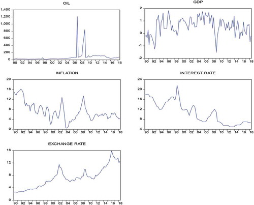
According to Figure 1 above, the plot of the oil price seem to be nonstationary with values revolving around zero line, though around 2006 and 2010, there is a large increase, which means by that time there was a lot of oil price volatility effect in the country. The plot of the interest rate seems to be non-stationary since it measured decreasing trends which started on the year 1999. On the other hand, the GDP series appears to have an irregular pattern throughout the sample period. The exchange rate series revealed an upward cyclical trend from 1990 onwards. This upward trend could be the result of democracy on the South African economy based on the country’s exchange rate as the country’s trade with other countries favours the economy. The Inflation series shows a disturbance between the years 2003 and 2005, which rotated around zero. Furthermore, the recession that happened in 2009 could have also influenced disturbances. By eye inspection, it is concluded that the variables seems to be nonstationary. The formal test for stationarity was then computed and the results are presented in Table 2 below.

Table 2. Stationarity test results

Variables	Level of test	ADF test statistic	p-value	PP test statistic	p-value	Conclusion
Oil	Level	−7.707	0.000	−7.821	0.000	Stationary
	1st Difference	−8.930	0.000	−52.828	0.000	Stationary
Interest rate	Level	−2.019	0.279	−1.702	0.428	Nonstationary
	1st Difference	−6.416	0.000	−5.873	0.000	Stationary
Inflation	Level	−2.929	0.045	−2.248	0.191	Nonstationary
	1st Difference	−5.085	0.000	−7.082	0.000	Stationary
GDP	Level	−5.327	0.000	−5.314	0.000	Stationary
	1st Difference	−8.901	0.000	−30.958	0.000	Stationary
Exchange rate	Level	−0.721	0.836	−0.907	0.783	Nonstationary
	1st Difference	−8.528	0.000	−8.528	0.000	Stationary

Table 2 above presents the summary of the results for the ADF and PP tests. The results revealed that oil price, inflation and GDP are stationary at level, while interest rate and exchange rate are nonstationary. However, all the variables became stationary at first difference. This means that the variables are integrated to order 1. The following Figure 2 presents the residual series plot of the variables.

Figure 2. Residual time series plots.

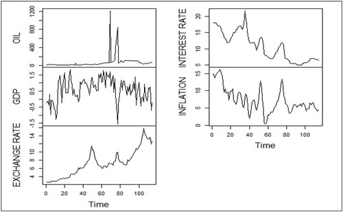
Figure 2 above illustrates the time series plots for the parameter estimations. The series are described by random/irregular, quick changes and are said to be unstable (volatile). The instability appears to change over time as well. For instance, oil price encounters a generally calm period from 1990 to 2006, whereas from 2006 to 2009, it shows an irregular volatility increase trend. On the other hand, exchange rate gives an increasing trend and interest rates a decreasing trend from 1990Q1 to 2018Q2. However, GDP provides similar periods of relative calm followed by increased volatility and drops throughout. The ARCH model was also computed to determine the presence of ARCH effects and the result are summarised in Table 3 below.

Table 3. Parameter estimation results of the ARCH model

Variables	Coefficient	Std. Error	z-Statistic	Prob.
GDP	61.401	2.408	25.504	0.000
Inflation	13.364	0.387	34.521	0.000
Interest rate	−16.253	0.342	−47.471	0.000
Exchange rate	−5.453	0.256	−21.296	0.000
C	148.302	4.787	30.983	0.000
Variance equation
C	82.995	91.566	0.906	0.365
	7.511	0.827	9.083	0.000

According to the results in Table 3, the ARCH (1) model is estimated as:

(6)

Equation (6)(6) illustrates the ARCH (1) model for oil price. According to the results, exchange rate and interest rate have a negative effect on oil price. However, GDP and Inflation have positive coefficients, suggesting that each 1% increase in GDP and inflation leads to an increase in oil price. The ARCH (1) effect is statistically significant with probability value less than the 5% level of significance. Therefore, the equation for oil price could be modelled using the GARCH and EGARCH techniques and the results are presented in Table 4 below.

Table 4. Parameter estimation results of the GARCH and EGARCH model

Model	Variables	Coefficient	Std. Error	z-Statistic	Prob.
GARCH	GDP	28.577	1.197	23.869	0.000
	Inflation	5.721	0.330	17.343	0.000
	Interest rate	−16.127	0.258	−62.615	0.000
	Exchange rate	−7.584	0.037	−206.236	0.000
	C	229.311	1.943	118.019	0.000
	Variance equation
	C	4.550	28.399	0.160	0.873
		11.838	0.770	15.369	0.000
		−0.0004	0.000	−0.818	0.413
EGARCH	GDP	−0.734	1.045	−0.703	0.482
	Inflation	−0.386	0.380	−1.014	0.311
	Interest rate	−7.228	0.414	−17.470	0.000
	Exchange rate	−2.029	0.259	−7.820	0.000
	C	125.816	3.318	37.921	0.000
	Variance equation
	Ω	−0.540	0.035	−15.386	0.000
		0.744	0.106	7.034	0.000
		−0.948	0.089	−10.678	0.000
		1.068	2.2E-104	4.8E+103	0.000

Table 4 presents the parameter estimation results of the GARCH and EGARCH model. Based on the results, the following GARCH (1, 1) model was formulated:

(7)

The GARCH (1, 1) model in Equation (7)(7) stated above is formed to determine relationships between the variables. According to the results, exchange rate and interest rate have negative values that propose a negative effect on oil price, while GDP and inflation suggest a positive effect. The GDP and inflation results propose that a 1% increase in GDP and inflation leads to an increase in oil price. However, the negative effect on interest rate and exchange rate led by its negative values implies that a 1% increase in interest rate and exchange rate may lead to a decrease in oil price. The results are in line with the study by Mirchandani (2013), who found similar results. However, in this case the interest value is negative and this may depress the foreign investors, as interest rate is one of the macroeconomic variables that has an effect on oil price volatility which attracts investors. In addition, the coefficients of the and β parameters are 11.838 and −0.000, respectively. The p-value of is found to be statistically significant, while the p-value of β is statistically insignificant. This means that there are ARCH effects and there are no GARCH effects. The sum of and β is found to be greater than 1. This means that the oil price in South Africa is volatile.

According to results in Table 4, the EGARCH model is formulated as:

(8)

The results for the EGARCH (1, 1) model presented in Equation (8)(8) shows a negative effect on all the macroeconomic variables (GDP, inflation, interest rate and exchange rate) on oil price. This implies that a 1% increase in the macroeconomic variables may lead to a decrease in oil price. The p-values for the coefficients are found to be statistically significant at 0.05 level of significance. The sum of coefficient is , which means that the oil price in South Africa is volatile. Table 5 summarise the diagnostic test results.

Table 5. Diagnostic test results

Oil Price		GARCH		EGARCH
Variable	Diagnostic tests	Statistics	p-value	Statistics	p-value
GDP	ARCH-LM	0.056	0.814	0.0003	0.987
	JB	3,508.024	0.000	2,940.838	0.000
	Box–Pierce test (R)	1.965	0.161	5.296	0.258
	Box–Ljung test (R^2)	2.178	0.156	5.540	0.236
Inflation	ARCH-LM	6.20e-05	0.099	4.81e-08	0.9998
	JB	15,692.89	0.000	6,255.761	0.000
	Box–Pierce test (R)	2.345	0.126	0.546	0.969
	Box–Ljung test (R^2)	2.407	0.120	0.569	0.966
Interest rate	ARCH-LM	0.009	0.926	0.003	0.956
	JB	25,507.08	0.000	12,060.64	0.000
	Box–Pierce test (R)	0.398	0.528	10.216	0.369
	Box–Ljung test (R^2)	0.408	0.523	10.501	0.033
Exchange rate	ARCH-LM	0.004	0.953	0.001	0.978
	JB	15,911.76	0.000	6,943.282	0.000
	Box–Pierce test (R)	0.090	0.764	1.538	0.820
	Box–Ljung test (R^2)	0.092	0.761	1.597	0.809

Table 5 above shows that all the macroeconomic variables on oil price have no ARCH errors since all the p-values for the ARCH-LM test are greater than the 0.05 level of significance. The results also revealed that all the macroeconomic variables show that the residuals are not normally distributed with p-values less than 0.05. The result of the Box–Ljung test (R²) shows that the residuals of these variables to oil price do not have serial correlation. Therefore, the GARCH and EGARCH models appear to be adequate to model the relationship between oil price volatility and macroeconomic variables.

5. Conclusion

The article modelled the oil price volatility and macroeconomic variables using the ARCH, GARCH and EGARCH models. The results revealed that all the macroeconomic variables are integrated to order 1. The ARCH (1) model revealed that the exchange rate and interest rate have a negative effect on oil price. The results also revealed that GDP and Inflation have positive coefficients, suggesting that each 1% increase in GDP and inflation leads to an increase in oil price. The ARCH model showed statistically significant results which means the mean equation could be fitted using GARCH technique, and the results are supported by Al-Raimony and El-Nader (2012).

The results of the GARCH (1, 1) model revealed that exchange rate and interest rate have negative values that propose a negative effect on oil price, while GDP and inflation suggest a positive effect. The results for GDP and inflation suggest that a 1% increase in GDP and inflation may lead to an increase in oil price. The results are supported by the study of Mpofu (2016), Mirchandani (2013), and Agnolucci (2009). The EGARCH (1, 1) model estimated results revealed that all the macroeconomic variables have a negative effect on the oil price. This implies that a 1% increase in these variables may lead to a decrease in oil price. The results are in line with the study by Ramzan et al. (2012). Both the symmetric and asymmetric techniques found that the South African oil prices are volatile.

Furthermore, in determining the model accuracy the diagnostic checks were examined using the normality test and the serial correlation method. However, the findings revealed that there is volatility among the macroeconomic variables and the dependent variable (oil price), and the article recommends that policy makers should have a view on the impact of oil price volatility on the South African economy. The article also recommends similar investigations should be undertaken in order to increase the validity and consistency of the results.

Additional information

Funding

The authors received no direct funding for this research.

Notes on contributors

Boitumelo Nnoi Yolanda Sekati

Boitumelo Nnoi Yolanda Sekati holds a Master of Commerce in Statistics and she is currently a PhD candidate at the Department of Business Statistics and Operations Research, North-West University. Her areas of interest include Econometrics, Multivariate Techniques and Time Series.

Johannes Tshepiso Tsoku

Johannes Tshepiso Tsoku is a Senior Lecturer at the Department of Business Statistics and Operations Research, North-West University. He holds a PhD in Statistics. His areas of interest include Econometrics, Applied Statistics, Multivariate Techniques and Time Series.

Lebotsa Daniel Metsileng

Lebotsa Daniel Metsileng holds a PhD in Statistics and poses a vast experience teaching the subject. He is a Senior Lecturer at the Department of Business Statistics and Operations Research, North-West University. His areas of interest include Multivariate Techniques, Econometrics and Time Series. He published several articles in international journals. He believes team goals are better scored than individual goals. He is more concerned about details and more results driven.

References

- Adelman, A. (2000). Determinants of growth and development of the Australian economy. Australian Journal of Economics, 14 (3),19–21,28, 34, 42.
- Agnolucci, P. (2009). Volatility in crude oil futures: A comparison of the predictive ability of GARCH and implied volatility models. Energy Economics, 31(2), 316–12. https://doi.org/10.1016/j.eneco.2008.11.001
- Al-Raimony, A. D., & El-Nader, H. M. (2012). The Sources of Stock Market Volatility in Jordan. International Journal of Economics and Finance, 4(11), 108. doi:10.5539/ijef.v4n11p108 11
- Aye, G. C., Dadam, V., Gupta, R., & Mamba, B. (2014). Oil price uncertainty and manufacturing production. Energy Economics, 43, 41–47. https://doi.org/10.1016/j.eneco.2014.02.004
- Baumohl, E., & Lyocsa, S. (2009). Stationarity of time series and the problem of spurious regression. Faculty of Business Economics in Kosice, University of Economics in Bratislava.
- Bollerslev, T. (1986). Generalized autoregressive conditional heteroscedasticity. Journal of Econometrics, 31(3), 307–327. https://doi.org/10.1016/0304-4076(86)90063-1
- Dickey, D. A., & Fuller, W. A. (1979). Distribution of the estimators for autoregressive time series with unit root. Journal of American Statistical Association, 74(366a), 427-431.
- Dunn, S., & Holloway, D. (2012). The pricing of crude oil. International Department September Quarter Bulletin, 65. Retrieved June, 2018, from https://www.rba.gov.au/publications/bulletin/2012/sep/pdf/bu-0912-8.pdf
- Guo, H., & Kliesen, K. L. (2005). Oil price volatility and US macroeconomic activity. Review-Federal Reserve Bank of St. Louis, 57(6), 669–683.
- Jin, G. (2008). The impact of oil price shock and exchange rate volatility on economic growth: A comparative analysis for Russia, Japan, and China. Research Journal of International Studies, 8(11), 98–111.
- Kutu, A. A., & Ngalawa, H. (2017). Modelling exchange rate volatility and global shocks in South Africa. Acta Universitatis Danubius, 13(3), 178–193.
- Lipsky, J. (2009, March 18). Economic shifts and oil price volatility. First deputy managing director of the international monetary fund at the 4th OPEC international seminar, Vienna.
- Milonas, N. T., & Henker, T. (2001). Price spread and convenience yield behaviour in the international oil market. Applied Financial Economics, 11(1), 23–36. https://doi.org/10.1080/09603100150210237
- Mirchandani, A. (2013). Analysis of macroeconomic determinants of exchange rate volatility in India. International Journal of Economics and Financial Issues, 3(1), 172–179.
- Moroke, N. (2005). An application of Box-Jenkins transfer function analysis to consumption income relationship in SA [Master’s paper]. Department of statistics, NWU.
- Mpofu, T. R. (2016). The determinants of exchange rate volatility in South Africa (ERSA Working Paper). p. 604.
- Narayan, P., Kumar, P., & Narayan, S. (2007). Modelling oil price volatility. Energy Policy, 35(12), 6549–6553. https://doi.org/10.1016/j.enpol.2007.07.020
- Nelson, D. B. (1991). Conditional heteroskedasticity in asset returns: A new approach. Econometrica, 59(2), 347–370. https://doi.org/10.2307/2938260
- Phillips, P., & Perron, P. (1988). Testing for a unit root in time series regression. Biometrika, 75(2), 335–346. https://doi.org/10.1093/biomet/75.2.335
- Ramzan, S., Ramzan, S. Z., & Zahid, F. M. (2012). Modelling and forecasting exchange rate dynamics in Pakistan using ARCH family of models. Electronic Journal of Applied Statistical Analysis, 5(1), 15–29. https://doi.org/10.1285/i20705948v5n1p15
- Reider, R. (2009). Volatility forecasting I: GARCH models. Retrieved October/August 1, 2018, from http://cims.nyu.edu/almgren/timeseries/Vol_Forecast1.pdf
- Sadorsky, P. (2006). Modelling and forecasting petroleum futures volatility. Energy Economics, 28(4), 467–488. https://doi.org/10.1016/j.eneco.2006.04.005
- Sahu, S. K., Beig, G., & Sharma, C. (2008). Decadal growth of black carbon emissions in India. Geophysical Research Letters, 35(2), 1-5. https://doi.org/10.1029/2007GL032333
- Taylor, S. (1986). Modelling financial time series. John Wiley and Sons.
- Tsay, R. (2005). Analysis of financial time series (2nd ed.). John Wiley & Sons.
- Wakeford, J. J. (2008). The impact of oil price shock on the South Africa macroeconomic, history and prospects. SARB conference.
- Wei, Y., Wang, Y., & Huang, D. (2010). Forecasting crude oil market volatility: Further evidence using GARCH-class models. Energy Economics, 32(6), 1477–1484. https://doi.org/10.1016/j.eneco.2010.07.009