Impact of exchange rate on uncertainty in stock market: Evidence from Markov regime-switching GARCH family models

Abstract

We employ the Markov Regime-Switching GARCH (MRS- GARCH) family models under the normal, Student’s t-, and GED distributions to measure the uncertainty of the industry index returns (IIR) of Tehran Stock Exchange over the period of 2013–2019. The models distinguish between two different regimes in both conditional mean and conditional variance. The results show that the MRS-EGARCH-in-mean (MRS-EGARCH-M) models under GED and Student’s t-distributions have the best performance to model the IIR volatility. We find evidence of regime-switching behaviour in Iran’s stock market. After removing the forecastable component (expected variation) from the best fitted models, we measure the time series of the IIR uncertainty (unforecastable component) and estimate the impact of exchange rate fluctuations on them using an autoregressive distributed lag (ARDL) model. We find that foreign exchange rate fluctuations have a significant and distinct impact on the IIR uncertainty across various regimes. The results show that the exchange rate generally has a negative and positive impact on the IIR uncertainty for export and import-oriented industries, respectively, under both regimes.

Keywords:

• uncertainty
• stock market
• Markov regime-switching

PUBLIC INTEREST STATEMENT

Uncertainty and risk are important components of investing in almost all financial markets including the stock market. Therefore, to make informed investments, uncertainty and risk need to be measured. In this paper, we develop a new model which measures risk more accurately. More specifically, we study the impact of exchange rate risk on the performance of different industries in the stock market. We also show that our model is superior to the previous models.

1. Introduction

Measurement of uncertainty, which is an amorphous concept in financial markets, is major concern for financial researchers. Recently, some studies suggest that in order to measure uncertainty accurately, it is necessary first to remove the common or forecastable component of the variation, and then proceed to the computation of the uncertainty indicator (Gilchrist et al., 2014). Uncertainty in a series is defined as the volatility of a purely unforecastable error of that series. The current value of time series depends on their previous values, with some lag, and random shocks. In financial markets, volatility estimations are common proxies for uncertainty (Caporale et al., 2015; Chuliá et al., 2017). In order to measure uncertainty, it is necessary to remove the forecastable component estimated from the variation of the best fitted model (Chuliá et al., 2017; Jurado et al., 2015).

In econometrics literature, the autoregressive integrated moving average (ARIMA) model with generalized autoregressive conditional heteroscedasticity (GARCH) processes is a popular model for measuring uncertainty (Ho et al., 2013). GARCH family models have been used to measure uncertainty of economic and financial variables such as inflation (e.g., Conrad & Hartmann, 2019; Daniela et al., 2014; Hartmann et al., 2017), oil price (e.g., Alsalman, 2016; Kocaaslan, 2019; Rahman & Serletis, 2012; Wang et al., 2017), and exchange rate (Caporale et al., 2015; Smallwood, 2019).

One major problem of the standard GARCH model is that it assumes that the conditional volatility follows only one regime over the entire period (Shi & Feng, 2016). To solve this Hamilton (1985, 1989)) proposed Markov Regime-Switching (MRS) models to allow for parameters to transit between state spaces. Recently, many studies have incorporated MRS specification into GARCH framework known as MRS-GARCH models (e.g., Gao et al., 2018; Naeem et al., 2019; Shi & Feng, 2016; Zhang et al., 2019; Zolfaghari & Sahabi, 2017). These models have been extensively examined on stock markets (e.g., Abounoori et al., 2016; Shi & Feng, 2016; Zhipeng & Shenghong, 2018).

In this paper, we use the MRS-GARCH family models to model the volatility of the Industry Index Returns (IIR) of Tehran Stock Exchange (TSE)) and to measure the IIR uncertainty over the period of 2013–2019.¹ MRS-GARCH models distinguish between two different regimes in both the conditional mean and the conditional variance of the IIR. We then compare the performance of these models with those of ARMA-GARCH family models under the normal, Student’s t-, and GED distributions.² Based on likelihood ratio test ($\mathrm{L}{\mathrm{R}}_{\mathrm{P}\mathrm{G}}$) suggested by Garcia and Perron (1996), we choose the best fitted models from both groups (MRS-GARCH and ARMA-GARCH family models). Our findings indicate that MRS-EGARCH-M model under GED and Student’s t-distribution outperforms other models. After removing the forecastable component from the best fitted models, we measure the IIR uncertainty.

We also investigate if the exchange rate dose influence the IIR uncertainty. Many economists have suggested a significant relationship between the stock markets and exchange rates (e.g., Abouwafia & Chambers, 2015; Bahmani-Oskooee & Saha, 2016; Roubaud & Arouri, 2018; Singhal et al., 2019; Tunc & Solakoglu, 2017). There is a fairly sizable literature showing that exchange rate movements affect stock prices. Our finding (based on ARDL model) show that foreign exchange rate has a significant impact on the IIR uncertainty that varies across different regimes.

The contribution of this paper is threefold. First, we propose an improved method to measure the return uncertainty in the stock market. In previous studies (e.g., Buth et al., 2015; Caporale et al., 2015; Kido, 2016), the uncertainty had been measured through the standard GARCH models. In this study, we improve these models using several distributions (the normal, Student’s t-, GED distributions) and take into account the feedback and leverage effects. Our second and main contribution is that we use the MRS-GARCH family models under different regimes. The results show that MRS-GARCH family models have better performance than benchmark models indicating that regime switching capability is an important feature to model the IIR uncertainty. Last, we examine the impact of the exchange rate fluctuations on the IIR uncertainty across two different regimes.

2. Methodology

2.1. ARMA-GARCH models

Some studies report that standard GARCH model is the best to model the stock market volatility (Lim & Sek, 2013). However, others (e.g., Zolfaghari & Sahabi, 2017, 2019) show that asymmetric GARCH model improves the performance of measuring conditional variance. Therefore, in addition to the standard GARCH model, we use the specifications of the GARCH-M (in mean), EGARCH, EGARCH-M (in mean), the IGARCH, and IGARCH-M (in mean) models. All models in our specification allow for change in the series of log-returns according to heteroskedastic diffusion:

• $r_t={\mu }_t+{ϵ}_t,h_{\mathrm{t}}=\omega +\sum _{i=1}^p{\alpha }_i{ϵ}_{t-i}^2+\sum _{j=1}^q{\beta }_j{h}_{\mathrm{t}-j}$ for GARCH model

• $r_t={\mu }_t+\lambda {\sqrt{h}}_t+{ϵ}_t,h_{\mathrm{t}}=\omega +\sum _{i=1}^p{\alpha }_i{ϵ}_{t-i}^2+\sum _{j=1}^q{\beta }_j{h}_{\mathrm{t}-j}$ for GARCH-M model

• $r_t={\mu }_t+{ϵ}_t,ln\left(h_{\mathrm{t}}\right)=\omega +\sum _{p=1}^P{\alpha }_p\left(\left|\frac{{ϵ}_{t-p}}{{\sqrt{h}}_{t-q}}\right|-\sqrt{\frac{2}{\pi }}\right)+\sum _{o=1}^O{\gamma }_o\frac{{ϵ}_{t-o}}{{\sqrt{h}}_{t-o}}+\sum _{q=1}^Q{\beta }_q\mathrm{l}\mathrm{n}\left(h_{\mathrm{t}-q}\right)$for EGARCH model

• $r_t={\mu }_t+\lambda {\sqrt{h}}_t+{ϵ}_t,ln\left(h_{\mathrm{t}}\right)=\omega +\sum _{p=1}^P{\alpha }_p\left(\left|\frac{{ϵ}_{t-p}}{{\sqrt{h}}_{t-q}}\right|-\sqrt{\frac{2}{\pi }}\right)+\sum _{o=1}^O{\gamma }_o\frac{{ϵ}_{t-o}}{{\sqrt{h}}_{t-o}}+\sum _{q=1}^Q{\beta }_q\mathrm{l}\mathrm{n}\left(h_{\mathrm{t}-q}\right)$for EGARCH-M model

• $r_t={\mu }_t+{ϵ}_t{h}_{\mathrm{t}}=\omega +{\beta }_1{h}_{\mathrm{t}-1}+\left(1-{\beta }_1\right){ϵ}_{t-1}^2$ for IGARCH models

• $r_t={\mu }_t+\lambda {\sqrt{h}}_t+{ϵ}_t,h_{\mathrm{t}-1}=\omega +{\beta }_1{h}_{\mathrm{t}-1}+\left(1-{\beta }_1\right){ϵ}_{t-1}^2$ for IGARCH-M models

in which, ${\mu }_t$ is ARIMA mean equation, and $h_{\mathrm{t}}$ is conditional variance (i.e. volatility).³

Evidence suggests that the financial time series are rarely Gaussian but typically leptokurtic, and exhibits fat-tail behaviour (Zolfaghari & Sahabi, 2017).

2.2. MRS-GARCH models

One issue with GARCH models is that they tend to overestimate volatility forecasts, particularly during periods of high volatility, which is due to the high degree of persistence implied by GARCH model. This persistence could be derived from structural changes in the variance process (Hamilton & Susmel, 1994), and can lead to weak forecasts (Birtoiu & Dragu, 2012). In order to overcome this issue, an MRS process can be employed to model the changes in parameters. The MRS model has the advantage of using the estimation of varying regime-switching probabilities of being in a particular regime instead of a linear model that is estimated for each regime separately (Haas et al., 2006). Regime-switching models are characterized by the possibility for some or all parameters to change across several states according to a Markov process, which is governed by a state variable $S_t$. Regime-switching models draw the current value of the variable from a set of possible distributions based on the most likely state that could have determined such an observation.

The transition probability represents the probability of switching from state $i$ at $t-1$ to state $j$ at $t$:

(1) $Pr\left(s_t=j\left|s_{t-1}=i\right.\right)=P_{ij}$(1)

If we assume, for simplicity, that there are only 2 states, the transition matrix⁴ can be written as:

(2) $P=\left(\begin{array}{cc}{\rho }_{11}& {\rho }_{21}\\ {\rho }_{12}& {\rho }_{22}\end{array}\right)=\left(\begin{array}{cc}\rho & 1-q\\ 1-\rho & q\end{array}\right)$(2)

In our study, we let $\left\{S_t\right\}$ follow a two-state first-order Markov process with time varying transition probabilities:

(3) $\begin{array}{rl}& Pr\left(S_t=1|S_{t-1}=1,r_t\right)=P_{t,}\\ & Pr\left(S_t=2|S_{t-1}=1,r_t\right)=1-P_{t,}\\ & \mathrm{P}\mathrm{r}\left(S_t=1|S_{t-1}=2,r_t\right)=1-q_{t,}\\ & Pr\left(S_t=2|S_{t-1}=2,r_t\right)=q_t\end{array}$(3)

The probability of being in regime $i$ for $i=1,2$ depends on realizations in ${\tilde{r}}_t$ and $\left\{S_t\right\}$ only through $S_{t-1}$. For the time varying transition probabilities we assume:

(4) $\begin{array}{rl}& P_t=\mathrm{\Phi }\left(d_1+e_1.r_t\right),\\ & q_t=\mathrm{\Phi }\left(d_2+e_2.r_t\right)\end{array}$(4)

with $\mathrm{\Phi }\left(0\right)$ denoting the cumulative distribution function and $d_1,d_2,e_1,e_2$ representing parameters to be estimated from the data. A general form of the MRS-GARCH models can be written as:

(5) $r_t\left|{\varphi }_{t-1}\right.\text{~}\left\{\begin{array}{c}f\left({\theta }_t^{\left(1\right)}\right)withprobability{p}_{1t}\\ f\left({\theta }_t^{\left(2\right)}\right)withprobability\left(1-p_{1t}\right)\end{array}\right.$(5)

where,$f\left(\ast \right)$ stands for one of the possible conditional distributions used in the model (normal, Student’s-t, GED), ${\theta }_t^{\left(i\right)}$ is the vector of parameters in the $ith$ regime that characterizes the distribution,$p_{1t}=\mathrm{P}\mathrm{r}\left(s_t=1\left|{\varphi }_{t-1}\right.\right)$ is the ex-ante probability and ${\varphi }_{t-1}$is the information set at $t-1$.

The vector of time varying parameters $\theta$, can be written as a function of three components:

(6) ${\theta }_t^{\left(i\right)}=\left({\mu }_t^{\left(i\right)},h_t^{\left(i\right)},v_t^{\left(i\right)}\right)$(6)

where, ${\mu }_t^{\left(i\right)}=E\left(r_t\left|{\varphi }_{t-1}\right.\right)$ is the conditional mean, $h_t^{\left(i\right)}=Var\left(r_t\left|{\varphi }_{t-1}\right.\right)$ is the conditional variance, and $v_t^{\left(i\right)}$ is the shape parameter of the conditional distribution.

Therefore, there are four main input elements in a MRS-GARCH model: conditional mean, conditional variance, regime process and conditional distribution. The conditional mean is modelled as:

(7) $r_t={\mu }_t^{\left(i\right)}+{\epsilon }_t$(7)

where, i = 1, 2 (since we assume two regimes), ${\epsilon }_t={\eta }_t\sqrt{h_t}$ and ${\eta }_t\text{~}iid\left(0,1\right)$. The conditional variance, given the whole unobserved regime path ${\tilde{s}}_t=\left(s_t,s_{t-1},\dots \right)$ is $h_t^{\left(i\right)}=V\left({\epsilon }_t\left|{\tilde{s}}_t,{\varphi }_{t-1}\right.\right)$. Conditional variance follows GARCH(1,1):

(8) $h_t^{\left(i\right)}={\alpha }_0^{\left(i\right)}+{\alpha }_1^{\left(i\right)}{\epsilon }_{t-1}^2+{\beta }_1^{\left(i\right)}{h}_{t-1}$(8)

in which $h_{\mathrm{t}-1}$ is an average of past conditional variances. This simplification is due to the fact that the state-dependency of the past conditional variances of a GARCH model is infeasible in a regime-switching context. The reason is that the conditional variance would depend on the observable information set ${\varphi }_{\mathrm{t}-1}$, the current regime ${\mathrm{s}}_{\mathrm{t}}$ which determines the parameters, as well as all past states ${\tilde{\mathrm{s}}}_{\mathrm{t}-1}$.

In order to avoid this path-dependency Hamilton (1985, 1989), Cai (1994), Gray (1996), Dueker (1997), and Klaanssen (2002) advocate the use of the conditional expectation of the lagged variance as a proxy for the lagged variance. The MRS-GARCH model proposed by Klaanssen (2002) has two main advantages compared to previous models. First, it allows for higher flexibility in capturing the persistence of shocks to volatility. Second, similar to standard GARCH models, direct expressions for the multi-step ahead volatility forecasts exist. Klaanssen (2002) recommend using the conditional expectation of the lagged conditional variance with an extended information set. His model also integrates out the past regimes by taking into account the current ones using the following specification for the conditional variance:

(26) $h_t^{\left(i\right)}={\alpha }_0^{\left(i\right)}+{\alpha }_1^{\left(i\right)}{\epsilon }_{t-1}^2+{\beta }_1^{\left(i\right)}{E}_{t-1}\left[h_{t-1}^{\left(i\right)}\left|s_t\right.\right]$(26)

in which the conditional expectation is defined as:

(27) $E_{t-1}\left[h_{t-1}^{\left(i\right)}\left|s_t\right.\right]={\tilde{p}}_{ii.t-1}\left[{\left(h_{t-1}^{\left(i\right)}\right)}^2+h_{t-1}^{\left(i\right)}\right]+{\tilde{p}}_{ji.t-1}\left[{\left({\mu }_{t-1}^{\left(j\right)}\right)}^2+h_{t-1}^{\left(j\right)}\right]-{\left[{\tilde{p}}_{ii.t-1}{\mu }_{t-1}^{\left(i\right)}+{\tilde{p}}_{ji.t-1}{\mu }_{t-1}^{\left(j\right)}\right]}^2$(27)

and the probabilities are computed as:

(28) ${\tilde{p}}_{ji.t}=Pr\left(s_t=j\left|s_{t+1}=i,\right.{\mathrm{\Omega }}_{t-1}\right)=\frac{{\tilde{p}}_{ji}\mathrm{P}\mathrm{r}(s_t=j\left|{\mathrm{\Omega }}_{t-1})-p_{ji}{p}_{j,t}\right.}{\mathrm{P}\mathrm{r}(s_t=j\left|{\mathrm{\Omega }}_{t-1})p_{i,t+1}\right.}withi,j=1,2$(28)

3. Empirical analysis and discussion

3.1. Data description

In this study, we focus on Tehran Stock Exchange (TSE) over the period of 1 September 2013 to 27 February 2019. Most of the previous studies have been conducted on developed, large, deep and low-volatility stock markets. TSE total market capitalization is nearly one-third of the country’s GDP, and a wide range of stocks, derivatives, and debt securities are traded on this exchange. The stock market data and exchange rate (US Dollar (USD)/Iranian Rial (IRR)) are obtained from TSE and the Central Bank of Iran, respectively.⁵

We use the daily index return for the 17 big industries (where there are at last three listed companies) of the TSE, industry index returns (IIR). For each industry, the daily return of industry index is computed as ${\mathrm{r}}_{\mathrm{t}}=\mathrm{l}\mathrm{n}\left(\frac{{\mathrm{p}}_{\mathrm{t}}}{{\mathrm{p}}_{\mathrm{t}-1}}\right)\times 100$, where, ${\mathrm{p}}_{\mathrm{t}}$ is the industry index closing value on day $t$. Table 1 reports some characteristics of selected industries, including average number of the listed companies and their share of the total market value. Among industries, the Chemical and Basic metals have the highest market share (22.4% and 14.21%, respectively). Also, the Cement and Chemical industries have the largest number of listed companies.

Table 1. Descriptive statistics of the IIR

Industry	Share of total market capitalization (%)	No. of listed companies	Mean	St.dev.	Skewness	Kurtosis	Jarque-Bera P- value	ADF	PP	KPSS
Investment	1.95	15	0.148	1.056	0.470337	4.493553	0.012	−24.1	−24.9	0.10
Chemical	22.04	28	0.217	1.104	0.915198	10.23411	0.000	−24.2	−24.6	0.12
Bank	6.89	9	0.142	1.053	0.67145	5.683714	0.005	−15.8	−25.1	0.24
Medication	3.9	27	0.183	0.725	2.129234	13.22147	0.000	−19.2	−21.8	0.19
Machinery	0.46	10	0.125	0.937	2.294896	23.9831	0.000	−10.9	−29.3	0.33
Metal products	0.36	6	0.150	1.640	2.027765	17.53797	0.000	−27.2	−28.3	0.20
Oil products	8.61	8	0.195	1.692	5.828696	96.44304	0.000	−29.3	−29.9	0.51
Auto	3.92	25	0.128	1.724	0.406648	3.736523	0.026	−16.9	−24.4	0.17
Basic metals	14.21	22	0.149	1.193	0.546614	4.894231	0.011	−24.9	−25.3	0.16
Food	0.99	16	0.166	1.401	4.183721	63.23804	0.000	−19.1	−29.4	0.10
Ceramic Tile	0.10	6	0.194	1.252	2.566876	24.36321	0.000	−14.9	−27.33	0.15
Sugar	0.36	10	0.234	1.568	1.869047	16.62206	0.000	−23.4	−24.5	0.44
Rubber	0.31	7	0.204	1.801	11.69757	264.523	0.000	−32.4	−32.5	0.41
Cement	1.34	30	0.112	1.531	0.963421	15.62435	0.000	−25.51	−26.9	0.16
Mining	6.80	10	0.172	1.469	−0.192789	16.46637	0.000	−25.4	−25.9	0.14
Real Estate	0.55	11	0.084	1.097	0.367475	4.481984	0.015	−22.5	−22.9	0.11
Insurance	0.57	6	0.101	1.365	0.942791	14.69021	0.000	−24.55	−26.1	0.17
USD/IRR rate return			0.087	1.67	−.711	42.2927	0.000	−21.707	−39.22	0.659

Note: The IIR are calculated based on $\mathrm{l}\mathrm{n}\left(\frac{{\mathrm{p}}_{\mathrm{t}}}{{\mathrm{p}}_{\mathrm{t}-1}}\right)\times 100$. Values of Skewness for most industries is positive, which show low probability of large decreases in the IIR. Given the inflationary conditions in the Iran economy and the support of institutional investors for the stock market (who are the main market player), this is a reasonable observation. According to the Jarque-Bera statistics, the IIR do not follow the normal distribution.

In columns 4 to 11 of Table 1, the descriptive statistics of the IIRs have been provided. Positive skewness suggests low probability of large decreases in the IIR during the study period. High kurtosis implies that extreme index changes occur frequently. The Jarque and Bera (1980) statistics, which measure the normality of the distribution using both skewness and kurtosis statistics, show that we can reject the null hypothesis of normality for all return series at conventional significant levels.

Both Dicky and Fuller (1979) and Phillips and Perron (1988) statistics indicate no evidence of a unit root in the IIR. The test statistics of Kwiatkowski et al. (1992) cannot reject the null hypothesis of stationary, therefore, we use ARMA instead of ARIMA.

The bottom row of Table 1 show summary statistics of the USD/IRR rate returns. According to the Skewness, Kurtosis and Jarque-Bera P-value, exchange rate changes do not follow a normal distribution.

3.2. Measuring the IIR uncertainty

The first step to measure the uncertainty is modelling the forecastable component of IIR. In order to do that, we take the following five steps:

Step 1: Estimating the ARMA model

IIR volatility modelling includes the specification of the ARMA ($p,q$) model corresponding to the stages described by Box and Jenkins (1970). To identify the best fitted model, we apply the Schwarz Information Criterion (SIC). This criterion represents a trade-off between “fit” measured by the log likelihood value and “parsimony” measured by the number of free parameters. Table 2 shows the best fitted ARMA model for the IIR. According to Table 2, the estimated parameters of ARMA are significant at the level of 1% for all industry indexes.

Table 2. ARMA model to the IIR

Industry	Model	Model Structure of the IIR	I Industry	Model	Model Structure of the IIR
Investment	ARMA(1,0)	${\hat{y}}_t=0.001+0.35y_{t-1}$(13.6) (3.37)	Food	ARMA(2,0)	${\hat{y}}_t=0.001+0.22y_{t-1}+0.11y_{t-2}$(3.8) (7.7) (2.01)
Chemical	ARMA(1,2)	${\hat{y}}_t=0.002+0.93y_{t-1}-0.57u_{t-1}-0.28u_{t-2}$(−7.34) (−9.42) (18.38) (3.53)	Ceramic Tile	ARMA(1,1)	${\hat{y}}_t=0.001+0.31y_{t-1}+0.05u_{t-1}$(1.64) (10.5) (3.6)
Bank	ARMA(3,1)	${\hat{y}}_t=0.001-0.51y_{t-1}+0.23y_{t-2}+0.06y_{t-3}+0.89u_{t-1}$(28.8) (1.99) (6.6) (−12.6) (3.2)	Sugar	ARMA(1,0)	${\hat{y}}_t=0.002+0.37y_{t-1}$(13.97) (3.51)
Medication	ARMA(1,2)	${\hat{y}}_t=0.001+0.91y_{t-1}-0.44u_{t-1}-0.25u_{t-2}$(−7.39) (−11.49) (37.45) (2.84)	Rubber	ARMA(1,1)	${\hat{y}}_t=0.002+0.97y_{t-1}-0.95u_{t-1}$(−41.34) (59.8) (1.98)
Machinery	ARMA(1,0)	${\hat{y}}_t=0.001+0.32y_{t-1}$(11.7) (3.15)	Cement	ARMA(1,3)	${\hat{y}}_t=0.01+0.95y_{t-1}-0.45u_{t-1}-0.3u_{t-2}-0.08u_{t-3}$(−2.7) (−8.6) (−10.2) (30.6) (1.7)
Metal Products	ARMA(1,0)	${\hat{y}}_t=0.001+0.24y_{t-1}$(8.47) (2.46)	Mining	ARMA(1,0)	${\hat{y}}_t=0.001+0.31y_{t-1}$(11.01) (2.94)
Oil Products	ARMA(1,0)	${\hat{y}}_t=0.001+0.17y_{t-1}$(5.85) (3.39)	Real State	ARMA(1,0)	${\hat{y}}_t=0.001+0.41y_{t-1}$(15.47) (1.72)
Auto	ARMA(0,1)	${\hat{y}}_t=0.001+0.36u_{t-1}$(13.5) (2.1)	Insurance	ARMA(1,2)	${\hat{y}}_t=0.001+0.89y_{t-1}-0.58u_{t-1}-0.19u_{t-2}$(−5.64) (−11.74) (22.42) (0.99)
Basic Metals	ARMA(1,2)	${\hat{y}}_t=0.001+0.91y_{t-1}-0.58u_{t-1}-0.25u_{t-2}$(−6.25) (−8.36) (15.03) (2.44)

Notes: $y_t$ is the value of IIR and $u_t$ is random shocks. Also, the t-statistics are shown below the estimates in parentheses.

Step 2: Estimating the GARCH family models

After estimating ARMA model for the IIR, the “ARCH effect” is tested for the IIR. The results show that most industries (except for six of them i.e. Machinery, Metal products, Food, Ceramic tile, Oil and Rubber), have ARCH effect based on F and ${\chi }^2$ statistics. Therefore, these six industries are transferred to the third step, and the rest are modelled based on four GARCH family models under the normal, Student’s-t, and GED distributions. Table 3 shows the conditional mean and variance models for the Investment industry.

Table 3. The conditional mean and variance models for the Investment industry

Model	Distribution	Conditional mean	Conditional variance
GARCH	Normal	${\hat{y}}_t=0.003+1.03y_{t-1}-0.58u_{t-1}-0.39u_{t-2}$(−13.9) (−21.3) (733.2) (2.4)	${\hat{h}}_t=0.001+0.24{\epsilon }_{t-1}^2+0.69h_{t-1}$(23.1) (8.4) (6.8)
	t	${\hat{y}}_t=0.001+0.95y_{t-1}-0.51u_{t-1}-0.35u_{t-2}$(−12.6) (−16.8) (58.1) (1.94)	${\hat{h}}_t=0.001+0.16{\epsilon }_{t-1}^2+0.82h_{t-1}$(31.3) (5.8) (3.31)
	GED	${\hat{y}}_t=0.001+0.95y_{t-1}-0.51u_{t-1}-0.35u_{t-2}$(13.5-) (17.19-) (62.6) (1.75)	${\hat{h}}_t=0.001+0.17{\epsilon }_{t-1}^2+0.79h_{t-1}$(23.4) (5.2) (3.7)
GARCH-M	Normal	${\hat{y}}_t=0.001+1.001y_{t-1}-0.58u_{t-1}+0.39u_{t-2}+0.13\sigma$(1.28) (−13.91) (−21.2) (656.5) (0.87)	${\hat{h}}_t=0.001+0.24{\epsilon }_{t-1}^2+0.69h_{t-1}$(22.1) (8.1) (6.7)
	t	${\hat{y}}_t=0.01+0.95y_{t-1}-0.50u_{t-1}-0.35u_{t-2}+0.03\sigma$(0.38) (−12.4) (−16.3) (53.5) (0.01)	${\hat{h}}_t=0.001+0.17{\epsilon }_{t-1}^2+0.81h_{t-1}$(30.8) (5.8) (3.3)
	GED	${\hat{y}}_t=0.001+0.95y_{t-1}+0.51u_{t-1}+0.36u_{t-2}+0.07\sigma$(0.9) (13.4) (17.1) (56.1) (1.37)	${\hat{h}}_t=0.001+0.18{\epsilon }_{t-1}^2+0.78h_{t-1}$(21.9) (52.1) (3.8)
EGARCH	Normal	${\hat{y}}_t=0.001+1.03y_{t-1}-0.59u_{t-1}-0.39u_{t-2}$(−14.3) (−22.1) (795.5) (1.64)	$ln{\hat{h}}_t=-1.5+0.42\left|\frac{{\epsilon }_{t-1}}{{\sigma }_{t-1}}\right|+0.04\frac{{\epsilon }_{t-1}}{{\sigma }_{t-1}}+0.88ln{h}_{t-1}$(53.3) (2.9) (12.9) (−8.3)
	t	${\hat{y}}_t=0.001+0.95y_{t-1}-0.51u_{t-1}-0.35u_{t-2}$(−12.9) (−17.1) (56.7) (2.44)	$ln{\hat{h}}_t=-0.64+0.28\left|\frac{{\epsilon }_{t-1}}{{\sigma }_{t-1}}\right|+0.02\frac{{\epsilon }_{t-1}}{{\sigma }_{t-1}}+0.95ln{h}_{t-1}$(82.5) (1.3) (8.21) (−4.8)
	GED	${\hat{y}}_t=0.001+0.97y_{t-1}-0.55u_{t-1}-0.35u_{t-2}$(−14.7) (−24.1) (124.5) (1.02)	$ln{\hat{h}}_t=-0.31+0.29\left|\frac{{\epsilon }_{t-1}}{{\sigma }_{t-1}}\right|-0.02\frac{{\epsilon }_{t-1}}{{\sigma }_{t-1}}+0.99ln{h}_{t-1}$(615.6) (−1.02) (12.4) (52.49)
EGARCH-M	Normal	${\hat{y}}_t=-0.21+0.99y_{t-1}-0.59u_{t-1}-0.38u_{t-2}+0.13\sigma$(1.65) (−15.07) (−22.5) (1677.7) (0.04)	$ln{\hat{h}}_t=-1.49+0.41\left|\frac{{\epsilon }_{t-1}}{{\sigma }_{t-1}}\right|+0.05\frac{{\epsilon }_{t-1}}{{\sigma }_{t-1}}+0.89ln{h}_{t-1}$(52.5) (3.1) (12.5) (−8.1)
	t	${\hat{y}}_t=0.001+0.95y_{t-1}-0.51u_{t-1}-0.36u_{t-2}+0.02\sigma$0.37)) (−12.8) (−16.8) (53.4) (2.06)	$ln{\hat{h}}_t=0.66+0.29\left|\frac{{\epsilon }_{t-1}}{{\sigma }_{t-1}}\right|+0.03\frac{{\epsilon }_{t-1}}{{\sigma }_{t-1}}+0.95ln{h}_{t-1}$(80.3) (1.22) (8.1) (4.8)
	GED	${\hat{y}}_t=0.001+0.95y_{t-1}-0.51u_{t-1}-0.36u_{t-2}+0.13\sigma$(1.48) (−13.2) (−16.8) (51.1) (1.28)	$ln{\hat{h}}_t=-1.07+0.35\left|\frac{{\epsilon }_{t-1}}{{\sigma }_{t-1}}\right|+0.04\frac{{\epsilon }_{t-1}}{{\sigma }_{t-1}}+0.92ln{h}_{t-1}$(48.9) (1.58) (7.7) (−5.1)
IGARCH	Normal	${\hat{y}}_t=0.02+0.99y_{t-1}-0.57u_{t-1}-0.32u_{t-2}$(−19.9) (−39.1) (639.2) (9.4)	${\hat{\sigma }}_t^2=0.01{\epsilon }_{t-1}^2+0.99{\sigma }_{t-1}^2$(3759.2) (19.91)
	t	${\hat{y}}_t=0.25+0.99y_{t-1}-0.53u_{t-1}-0.34u_{t-2}$(−17.5) (−28.01) (7291.2) (5.56)	${\hat{\sigma }}_t^2=0.02{\epsilon }_{t-1}^2+0.98{\sigma }_{t-1}^2$(562.3) (6.7)
	GED	${\hat{y}}_t=0.16+0.99y_{t-1}-0.61u_{t-1}-0.31u_{t-2}$(−17.5) (−34.2) (665.5) (6.6)	${\hat{\sigma }}_t^2=0.01{\epsilon }_{t-1}^2+0.99{\sigma }_{t-1}^2$(84.6) (5.8)
IGARCH-M	Normal	${\hat{y}}_t=0.001+0.99y_{t-1}-0.61u_{t-1}-0.35u_{t-2}+0.98\sigma$(3.2) (−19.85) (−37.8) (5021) (1.95)	${\hat{\sigma }}_t^2=-0.01{\epsilon }_{t-1}^2+0.99{\sigma }_{t-1}^2$(2526.3) (−6.1)
	t	${\hat{y}}_t=0.05+0.99y_{t-1}-0.56u_{t-1}-0.36u_{t-2}+0.89\sigma$(3.3) (−19.8) (−31.2) (588) (5.9)	${\hat{\sigma }}_t^2=-0.01{\epsilon }_{t-1}^2+0.99{\sigma }_{t-1}^2$(1939.4) (−1.14)
	GED	${\hat{y}}_t=0.02+0.99y_{t-1}-0.58u_{t-1}-0.37u_{t-2}+0.47\sigma$(2.2) (−21.9) (−34.4) (920.1) (4.6)	${\hat{\sigma }}_t^2=0.01{\epsilon }_{t-1}^2+0.99{\sigma }_{t-1}^2$(1697.1) (0.26)

The above process was carried out for the other industry indexes, but due to the limited space of the paper, their detailed presentation (as in Table 3) is in the online Appendix. As illustrated in Table 3 (and results of other industry indexes), most parameters are significant at 1%, 5% or 10% levels. The estimates of individual parameters from different models are quite close.

Step 3: Estimating the MRS-GARCH family models

After estimating the ARMA-GARCH models, we estimate each of these models by Markov Regime-Switching GARCH models. The estimated parameters of the MRS-GARCH models for Investment industry are presented in Table 4. The models for other 10 industries are provided in Appendix (A).

Table 4. The conditional mean and variance models for the Investment industry under MRS method

Model	type	Distribution	${\mu }_1$	${\mu }_2$	${\lambda }_1$	${\lambda }_2$	${\mathbf{b}}_{01}$	${\mathbf{b}}_{02}$
GARCH	simple	Normal	−0.053	0.703			0.014	0.000
		t	0.737	−0.050			0.000	0.008
		GED	0.608	−0.090			0.000	0.003
	in-mean	Normal	−0.101	0.023	0.239	6.710	0.000	0.036
		t	0.412	0.085	0.803	−0.200	0.002	0.012
		GED	0.382	0.078	0.702	−0.210	0.001	0.014
EGARCH	simple	Normal	0.571	−0.030			−0.148	−0.317
		t	0.564	−0.030			−0.173	−0.333
		GED	0.604	−0.030			−0.172	−0.332
	in-mean	Normal	0.569	−1.770	−1.105	2.605	−0.494	−0.103
		t	1.068	−2.110	−1.943	3.070	−0.444	−0.286
		GED	1.174	−2.240	−2.009	3.322	−0.405	−0.290
IGARCH	simple	Normal	−0.157	0.016			0.001	0.126
		t	0.387	0.062			0.003	0.009
		GED	0.349	0.048			0.002	0.006
	in-mean	Normal	−0.144	0.015	0.290	−3.910	0.009	0.107
		t	0.478	0.069	0.382	−0.170	0.001	0.010
		GED	0.477	0.052	0.209	−0.130	0.001	0.003
Model	type	Distribution	${\mathbf{b}}_{11}$	${\mathbf{b}}_{12}$	${\mathbf{b}}_{21}$	${\mathbf{b}}_{22}$	${\mathbf{b}}_{31}$	${\mathbf{b}}_{32}$	${\mathbf{p}}_{11}$	${\mathbf{p}}_{22}$
GARCH	simple	Normal	0.183	0.092	0.743	0.896			0.89	0.93
		t	0.137	0.188	0.821	0.755			0.89	0.92
		GED	0.098	0.203	0.893	0.708			0.88	0.9
	in-mean	Normal	0.015	0.017	0.113	0.983			0.78	0.82
		t	0.137	0.146	0.642	0.773			0.74	0.81
		GED	0.106	0.156	0.745	0.746			0.74	0.8
EGARCH	simple	Normal	−0.093	0.243	0.364	−0.120	0.984	0.991	0.91	0.96
		t	−0.036	0.281	0.319	−0.110	0.985	0.993	0.91	0.96
		GED	−0.052	0.261	0.329	−0.120	0.987	0.995	0.90	0.96
	in-mean	Normal	0.317	0.008	−0.381	0.253	0.863	0.601	0.75	0.70
		t	0.326	0.155	−0.367	0.250	0.889	0.544	0.64	0.72
		GED	0.328	0.119	−0.322	0.270	0.863	0.583	0.65	0.74
IGARCH	simple	Normal	0.785	0.005	0.215	0.995			0.63	0.81
		t	0.365	0.370	0.635	0.630			0.62	0.86
		GED	0.145	0.640	0.855	0.361			0.69	0.82
	in-mean	Normal	0.722	0.002	0.279	0.998			0.89	0.89
		t	0.221	0.258	0.779	0.742			0.85	0.87
		GED	0.103	0.237	0.897	0.763			0.86	0.87

In Table 4, columns ${\mu }_1$ and ${\mu }_2$show the conditional mean for regimes 1 and 2, respectively. Columns ${\lambda }_1$ and ${\lambda }_2$ show the “feedback effect” in the GARCH-M, IGARCH-M and EGARCH-M models. Parameters $b_{01}$ and $b_{02}$ are the intercept terms in the conditional variance equation for regimes 1 and 2, respectively. Parameters $b_{11}$ and $b_{12}$ are coefficients of ${\epsilon }_{\mathrm{t}-1}^2$in GARCH/IGARCH, GARCH-M/IGARCH-M models, and coefficients of $\left|\frac{{\epsilon }_{\mathrm{t}-1}}{\sqrt{{\mathrm{h}}_{\mathrm{t}-1}}}\right|$ in EGARCH, and EGARCH-M models for regimes 1 and 2, respectively. Parameters $b_{21}$ and $b_{22}$ are also coefficients of $h_{t-1}$ in GARCH/IGARCH, GARCH-M/IGARCH-M models and coefficients of $\frac{{\epsilon }_{\mathrm{t}-1}}{\sqrt{{\mathrm{h}}_{\mathrm{t}-1}}}$ (which are indicative of the leverage effect) in two models of EGARCH, and EGARCH-M for regimes 1 and 2, respectively. Finally, $b_{31}$ and $b_{32}$ are coefficients of $\mathrm{l}\mathrm{n}{h}_{t-1}$ in two models of EGARCH and EGARCH-M for regimes 1 and 2, respectively. In economic terms, regime 1 represents periods of low volatility with high returns (calm state), and regime 2 represents periods of high volatility with low returns (turbulent state).

Estimates of individual parameters from different models are not quite close. Specifically, both $p_{11}$ and $p_{22}$ are different in all models, suggesting that the expectations of staying in both regimes are different. Table 5 shows the conditional mean and variance models of six industries without the ARCH effect under MRS.

Table 5. Conditional mean and variance model of IIRs without the ARCH effect under MRS

Industry	${\mathbf{C}}_1$	${\mathbf{C}}_2$	${\mathbf{y}}_{1\left(\mathbf{t}-1\right)}$	${\mathbf{y}}_{2\left(\mathbf{t}-1\right)}$	${\mathbf{y}}_{1\left(\mathbf{t}-2\right)}$	${\mathbf{y}}_{2\left(\mathbf{t}-2\right)}$	${\mathbf{p}}_{11}$	${\mathbf{p}}_{11}$
Machinery	0.001	0.004	0.4	0.23			0.92	0.81
Metal products	0.001	0.007	0.3	−0.88
Oil products	0.001	0.01	0.35	−0.07
Food	0.0001	0.001	040	0.21	0.12	0.11	0.91	0.92
Ceramic Tile	0.001	0.003	0.62	0.14	0.09	−0.12	0.72	0.27
Rubber	0.001	0.01	0.37	0.01

According to the coefficients given in Table 5, three industries, Metal Products, Oil Products, and Rubber follow single regime and hence, do not display a switching behavior.

Step 4: Normality test

After estimating the ARMA-GARCH and MRS-GARCH family models, we examine the normality of distributions for the IIR in each of the estimated models using Jarque- Bera (1980) test. The results show that none of the models follow the normal distribution. Therefore, we choose the optimal model between the “Student’s-t” or “GED” distribution. To compare the models, due to restrictions of the Wald, Ordinary Likelihood Ratio, and Lagrange Multiplier tests (Garcia & Perron, 1996), we apply the likelihood ratio test ($\mathrm{L}{\mathrm{R}}_{\mathrm{P}\mathrm{G}}$) suggested by Garcia and Perron (1996). This test is computed as follows:

(9) $\mathrm{L}{\mathrm{R}}_{\mathrm{P}\mathrm{G}}=2\times \left|ln{L}_1-ln{L}_0\right|$

in which, $lnL$ is the log likelihood of the competing models.

Tables 6 and 7 show $\mathrm{L}{\mathrm{R}}_{\mathrm{P}\mathrm{G}}$ likelihood ratio statistics for ARMA-GARCH and MRS-GARCH family models.

Table 6. The results of $\mathbf{L}{\mathbf{R}}_{\mathbf{P}\mathbf{G}}$likelihood ratio for GARCH family models

Industry	GARCH						EGARCH
	Simple			In-mean			Simple			In-mean
	t	GED	Test statistics	t	GED	Test statistics	t	GED	Test statistics	t	GED	Test statistics
Investment	4005.0	4000.0	10.0	4006.0	4001.1	9.7	4007.9	4003.8	8.2	4008.7	4004.7	7.9
Chemical	4053.2	4050.2	6.0	4058.0	4055.5	4.9	4056.2	4055.3	1.8	4058.9	4059.0	0.3
Bank	4178.8	4166.3	25.0	4178.4	4168.7	19.4	4178.1	4168.3	19.5	4178.4	4168.7	19.4
Medication	4951.9	4921.0	61.9	4951.9	4921.0	61.8	4955.7	4930.7	50.1	4955.7	4930.8	49.7
Auto	3363.9	3348.3	31.2	3365.0	3348.4	33.2	3369.9	3353.3	33.2	3372.2	3354.0	36.4
Basic metals	3851.9	3849.0	5.8	3851.4	3847.6	7.5	3857.4	3853.3	8.3	3861.2	3858.2	6.0
Sugar	3697.9	3659.2	77.3	3698.5	3659.5	77.9	3703.1	3664.7	76.7	3704.6	3665.5	78.2
Cement	4624.4	4626.3	3.9	4624.4	4626.6	4.4	4639.0	4635.9	6.1	4639.0	4636.1	5.8
Mining	3865.8	3821.6	88.4	3865.8	3822.3	86.9	3836.6	3820.6	32.0	3836.8	3821.1	31.4
Real State	4089.8	4090.7	1.8	4089.9	4091.0	2.1	4092.7	4091.9	1.6	4092.6	4092.3	0.7
Insurance	3898.0	3865.1	65.8	3898.2	3865.1	66.3	3900.9	3877.9	45.9	3900.0	3878.0	44.1
Industry	IGARCH
	Simple			In-mean
	t	GED	Test statistics	t	GED	Test statistics
Investment	3993.7	3987.0	13.4	3878.0	3881.4	6.9
Chemical	4033.3	4033.6	0.5	3957.5	4037.4	159.8
Bank	4164.5	4149.1	30.8	4164.5	4149.1	30.8
Medication	4927.0	4901.7	50.8	4927.1	4901.7	50.9
Auto	3354.2	3336.9	34.6	3354.7	3336.9	35.6
Basic metals	3832.6	3846.2	27.3	3846.6	3846.8	0.3
Sugar	3675.8	3636.0	79.6	3631.8	3636.3	9.0
Cement	4610.1	4610.5	0.8	4610.1	4598.7	22.7
Mining	3837.1	3794.3	85.6	3837.1	3795.2	83.7
Real State	4082.6	4082.0	1.1	4083.0	4083.0	0.1
Insurance	3720.4	3855.5	270.2	3730.0	3855.1	250.1

Table 7. The results of the $\mathbf{L}{\mathbf{R}}_{\mathbf{P}\mathbf{G}}$ likelihood ratio for the MRS- GARCH family models

Industry	GARCH						EGARCH
	Simple			In-mean			Simple			In-mean
	t	GED	Test statistics	t	GED	Test statistics	t	GED	Test statistics	t	GED	Test statistics
Investment	−1593.8	−1599.4	11.1	−1584.1	−1587.3	6.4	−1596.8	−1599.9	6.1	−1557.3	−1556.4	2.0
Chemical	−1529.3	−1534.8	11.1	−1520.4	−1523.0	5.2	−1529.0	−1537.3	16.6	−1450.2	−1556.4	2012.
Bank	−1430.2	−1425.4	9.7	−1414.9	−1419.2	8.5	−1432.6	−1435.2	5.3	−1400.8	−1389.0	23.6
Medication	−630.0	−677.3	94.5	−610.4	−636.7	52.7	−650.0	−669.3	38.6	−570.9	−624.1	106
Auto	−2218.2	−2233.5	30.5	−2192.3	−2210.2	35.9	−2217.5	−2230.5	26.1	−2169.0	−2170.0	2.1
Basic metals	−1726.0	−1725.7	0.7	−1712.4	−1714.7	4.6	−1720.8	−1720.5	0.7	−1679.1	−1668.4	21.4
Sugar	−1881.6	−1898.7	34.3	−1845.1	−1878.8	67.5	−1886.9	−1913.4	53.1	−1834.9	−1785.6	98.6
Cement	−990.2	−994.8	9.3	−933.2	−943.5	20.4	−997.4	−999.4	4.0	−922.9	−898.2	49.2
Mining	−1719.5	−1726.3	13.6	−1705.7	−1716.1	20.9	−1742.0	−1763.0	42.0	−1676.0	−1681.1	10.1
Real State	−1507.0	−1509.9	5.7	−1486.8	−1488.7	3.8	−1515.5	−1515.3	0.4	−1478.5	−1470.2	16.4
Insurance	−1660.3	−1677.3	68.0	−1626.8	−1638.6	25.2	−1660.2	−1670.6	20.8	−1591.5	−1602.2	21.5
Industry	IGARCH
	Simple			In-mean
	t	GED	Test statistics	t	GED	Test statistics
Investment	−1596.7	−1596.1	0.6	−1593.8	−1598.6	9.5
Chemical	−1563.2	−1621.7	58.5	−1519.7	−1635.7	232
Bank	−1414.9	−1422.7	7.8	−1414.9	−1422.7	15.6
Medication	−685.2	−659.1	26.1	−614.4	−639.2	49.6
Auto	−2198.4	−2201.5	3.1	−2207.1	−2244.4	74.5
Basic metals	−1763.1	−1852.2	89.1	−1715.9	−1726.1	20.3
Sugar	−1859.8	−1892.2	32.4	−1809.8	−1892.1	164
Cement	−1708.3	−1098.2	89.9	−1809.8	−1722.0	87.7
Mining	−1721.1	−1726.5	10.8	−1719.4	−1735.5	32.1
Real State	−1499.4	−1496.3	3.0	−1491.5	−1501.2	19.4
Insurance	−1626.7	−1644.0	17.3	−1626.7	−1644.0	34.6

The results of the $\mathrm{L}{\mathrm{R}}_{\mathrm{P}\mathrm{G}}$likelihood ratio for ARMA-GARCH family models, as shown in Table 6, indicate that most IIRs follow EGARCH models (EGARCH and EGARCH-M).

The results of the $\mathrm{L}{\mathrm{R}}_{\mathrm{P}\mathrm{G}}$ likelihood ratio for the MRS- GARCH family models in Table 7 show that all selected IIRs follow EGARCH-M model. In fact, according to Table 7, all selected models have “feedback effect” in both regimes. In other words, the volatility of the IIR is significantly related to the IIR in both regimes. These effects are different and depend on the regime. Also, all selected models have “leverage effect” under both regimes, which means that the IIRs asymmetrically react to good and bad news.

Step 5: Choosing the best fitted models

In this step, we choose the best fitted model among the selected models in each industry (between the selected MRS-GARCH and ARMA-GARCH models) using the information criteria and the forecast accuracy measures. Information criteria include Akaike Information Criterion (AIC) and Schwarz Information Criterion (SIC). AIC and SIC offer a relative estimate of the information lost when a given model is used to represent the process that generates the data. The AIC penalizes the number of parameters less strongly than does the SIC. In addition to AIC and SIC, we use two forecast accuracy measures, root mean squared Error (RMSE) and mean absolute percentage error (MAPE). In general form, RMSE and MAPE are computed as follows:

(10) $\mathrm{R}\mathrm{M}\mathrm{S}\mathrm{E}=\sqrt{\frac{1}{\mathrm{n}}\sum _{\mathrm{i}=1}^{\mathrm{n}}{\left({\mathrm{y}}_{\mathrm{p}\mathrm{i}}-{\mathrm{y}}_{\mathrm{a}\mathrm{i}}\right)}^2},$(10)

(11) $\mathrm{M}\mathrm{A}\mathrm{P}\mathrm{E}=\frac{1}{\mathrm{n}}\sum _{\mathrm{i}=1}^{\mathrm{n}}\left|\frac{{\mathrm{y}}_{\mathrm{p}\mathrm{i}}-{\mathrm{y}}_{\mathrm{a}\mathrm{i}}}{{\mathrm{y}}_{\mathrm{a}\mathrm{i}}}\right|,$(11)

in which, ${\mathrm{y}}_{\mathrm{a}\mathrm{i}}\mathrm{a}\mathrm{n}\mathrm{d}{\mathrm{y}}_{\mathrm{p}\mathrm{i}}$represent the actual and predicted values, respectively. To investigate the out-of-sample accurate predictability, we conduct a 10-day ahead (two weeks) forecast for the index return of industries by selected models. The forecast accuracy measures (RMSE and MAPE) are used to examine the prediction accuracy of different models.

Table 8 shows the best fitted model of industries which have the ARCH effect, based on the information criteria and the forecast accuracy measures.

Table 8. The optimal model of industries that have the ARCH effect

Industry	ARMA-GARCH family model					MRS-GARCH family model
	Conditional variance model/Distribution	AIC	SIC	RMSE	MAPE	Conditional variance model/Distribution	AIC	SIC	RMSE	MAPE
Investment	EGARCH-M/t	−6.595	−6.616	3.153411	0.207755	EGARCH-M/t	−7.562	−7.570	1.084629	0.06896
Chemical	EGARCH-M/t	−6.709	−6.667	4.477946	0.085943	EGARCH-M/t	−7.397	−7.382	1.41845	0.024211
Bank	GARCH/t	−6.917	−6.883	1.337161	0.082905	EGARCH-M/GED	−7.299	−7.288	0.728011	0.066875
Medication	EGARCH/GED	−8.155	−8.117	31.1532	0.463816	EGARCH-M/t	−8.944	−8.940	12.95384	0.195033
Auto	EGARCH-M/t	−5.570	−5.536	128.2554	0.85348	EGARCH-M/GED	−8.584	−8.562	43.49717	0.31655
Basic metals	EGARCH-M/GED	−6.377	−6.334	70.60816	0.142823	EGARCH-M/GED	−7.758	−7.739	29.83139	0.046013
Sugar	EGARCH-M/t	−6.125	−6.091	52.3778	0.911583	EGARCH-M/GED	−7.952	−7.936	25.1705	0.405528
Cement	EGARCH/GED	−7.326	−7.224	1.527089	0.125249	EGARCH-M/GED	−7.119	−7.100	0.643428	0.054776
Mining	GARCH/t	−6.396	−6.370	48.70528	0.242795	EGARCH-M/t	−7.773	−7.762	15.83932	0.084725
Real State	EGARCH/t	−6.770	−6.740	4.709352	0.596981	EGARCH-M/GED	−7.432	−7.421	2.671704	0.317525
Insurance	EGARCH/t	−6.514	−6.475	11.53802	0.340857	EGARCH-M/t	−7.658	−7.642	6.609539	0.126027

Based on the AIC and SIC results in Table 8, the optimal model of all IIRs follow MRS- GARCH models. In fact, AIC and SIC value in MRS-GARCH models are lower than ARMA-GARCH models. As shown in Table 8, the MRS-GARCH models in all industries have the smaller RMSE and MAPE values compared with the ARMA-GARCH models. Indeed, the prediction errors of selected MRS-GARCH models are small based on two evaluation criteria. Therefore, we find strong evidence that MRS-GARCH models outperform the ARMA-GARCH family models in capturing the characteristics of the IIR series. Our findings indicate that MRS-EGARCH-M model under GED and Student’s t-distributions has better results than other MRS-GARCH models. Table 9 shows the characteristics of the optimal model for each industry.

Table 9. The optimal model of the IIR

Industry	Model	Regime	Equation	${\mathrm{p}}_{11}$	${\mathrm{p}}_{22}$	Duration
Investment	MRS-GARCH-M/t	1	${\hat{y}}_t=1.068-1.94\sigma ;ln{\hat{\sigma }}_t^2=-.44+0.32\left|\frac{{\epsilon }_{t-1}}{{\sigma }_{t-1}}\right|-0.37\frac{{\epsilon }_{t-1}}{{\sigma }_{t-1}}+0.88ln{\sigma }_{t-1}^2$	0.64	0.72	2.78	3.84
		2	${\hat{y}}_t=-2.11+3.07\sigma ;ln{\hat{\sigma }}_t^2=-.28+0.15\left|\frac{{\epsilon }_{t-1}}{{\sigma }_{t-1}}\right|+0.26\frac{{\epsilon }_{t-1}}{{\sigma }_{t-1}}+0.54ln{\sigma }_{t-1}^2$
Chemical	MRS-EGARCH-M/t	1	${\hat{y}}_t=-12.1+10.3\sigma ;ln{\hat{\sigma }}_t^2=0.35+0.01\left|\frac{{\epsilon }_{t-1}}{{\sigma }_{t-1}}\right|+0.06\frac{{\epsilon }_{t-1}}{{\sigma }_{t-1}}+0.03ln{\sigma }_{t-1}^2$	0.93	0.91	14.2	11.1
		2	${\hat{y}}_t=1.64-1.45\sigma ;ln{\hat{\sigma }}_t^2=0.23-0.22\left|\frac{{\epsilon }_{t-1}}{{\sigma }_{t-1}}\right|-0.3\frac{{\epsilon }_{t-1}}{{\sigma }_{t-1}}+0.22ln{\sigma }_{t-1}^2$
Bank	MRS-EGARCH-M/GED	1	${\hat{y}}_t=0.96-0.35\sigma ;ln{\hat{\sigma }}_t^2=-0.13+0.26\left|\frac{{\epsilon }_{t-1}}{{\sigma }_{t-1}}\right|-0.01\frac{{\epsilon }_{t-1}}{{\sigma }_{t-1}}+0.75ln{\sigma }_{t-1}^2$	0.95	0.96	20	25
		2	${\hat{y}}_t=1.5-3.04\sigma ;ln{\hat{\sigma }}_t^2=-0.81+0.14\left|\frac{{\epsilon }_{t-1}}{{\sigma }_{t-1}}\right|-0.44\frac{{\epsilon }_{t-1}}{{\sigma }_{t-1}}+0.42ln{\sigma }_{t-1}^2$
Medication	MRS-EGARCH-M/t	1	${\hat{y}}_t=0.005-0.12\sigma ;ln{\hat{\sigma }}_t^2=-0.07+0.05\left|\frac{{\epsilon }_{t-1}}{{\sigma }_{t-1}}\right|-0.14\frac{{\epsilon }_{t-1}}{{\sigma }_{t-1}}+0.99ln{\sigma }_{t-1}^2$	0.94	0.86	16.6	7.14
		2	${\hat{y}}_t=-0.66+1.86\sigma ;ln{\hat{\sigma }}_t^2=0.08-0.37\left|\frac{{\epsilon }_{t-1}}{{\sigma }_{t-1}}\right|+0.42\frac{{\epsilon }_{t-1}}{{\sigma }_{t-1}}+0.89ln{\sigma }_{t-1}^2$
Auto	MRS-EGARCH-M/GED	1	${\hat{y}}_t=0.87-0.37\sigma ;ln{\hat{\sigma }}_t^2=0.16+0.01\left|\frac{{\epsilon }_{t-1}}{{\sigma }_{t-1}}\right|-0.01\frac{{\epsilon }_{t-1}}{{\sigma }_{t-1}}+088ln{\sigma }_{t-1}^2$	0.93	0.91	14.2	11.1
		2	${\hat{y}}_t=-5.7+4.4\sigma ;ln{\hat{\sigma }}_t^2=0.33+0.10\left|\frac{{\epsilon }_{t-1}}{{\sigma }_{t-1}}\right|+0.17\frac{{\epsilon }_{t-1}}{{\sigma }_{t-1}}+0.14ln{\sigma }_{t-1}^2$
Basic metals	MRS-EGARCH-M/GED	1	${\hat{y}}_t=15.7-11.4\sigma ;ln{\hat{\sigma }}_t^2=0.59-0.01\left|\frac{{\epsilon }_{t-1}}{{\sigma }_{t-1}}\right|-0.04\frac{{\epsilon }_{t-1}}{{\sigma }_{t-1}}+0.01ln{\sigma }_{t-1}^2$	0.97	0.96	33.3	25
		2	${\hat{y}}_t=-3.4+5.4\sigma ;ln{\hat{\sigma }}_t^2=-0.99-0.03\left|\frac{{\epsilon }_{t-1}}{{\sigma }_{t-1}}\right|+0.14\frac{{\epsilon }_{t-1}}{{\sigma }_{t-1}}+0.96ln{\sigma }_{t-1}^2$
Sugar	MRS-EGARCH-M/GED	1	${\hat{y}}_t=0.38-0.11\sigma ;ln{\hat{\sigma }}_t^2=0.02+0.03\left|\frac{{\epsilon }_{t-1}}{{\sigma }_{t-1}}\right|-0.02\frac{{\epsilon }_{t-1}}{{\sigma }_{t-1}}+0.98ln{\sigma }_{t-1}^2$	0.92	0.78	12.5	4.5
		2	${\hat{y}}_t=0.31+0.17\sigma ;ln{\hat{\sigma }}_t^2=0.12+0.05\left|\frac{{\epsilon }_{t-1}}{{\sigma }_{t-1}}\right|-0.01\frac{{\epsilon }_{t-1}}{{\sigma }_{t-1}}+0.96ln{\sigma }_{t-1}^2$
Cement	MRS-EGARCH-M/GED	1	${\hat{y}}_t=-4.24+3.94\sigma ;ln{\hat{\sigma }}_t^2=0.25+0.013\left|\frac{{\epsilon }_{t-1}}{{\sigma }_{t-1}}\right|+0.20\frac{{\epsilon }_{t-1}}{{\sigma }_{t-1}}+0.07ln{\sigma }_{t-1}^2$	0.98	0.99	50	100
		2	${\hat{y}}_t=-0.88+2.05\sigma ;ln{\hat{\sigma }}_t^2=-0.19-0.23\left|\frac{{\epsilon }_{t-1}}{{\sigma }_{t-1}}\right|+0.87\frac{{\epsilon }_{t-1}}{{\sigma }_{t-1}}+0.92ln{\sigma }_{t-1}^2$
Mining	MRS-EGARCH-M/t	1	${\hat{y}}_t=-11.6+6.854\sigma ;ln{\hat{\sigma }}_t^2=0.96+0.06\left|\frac{{\epsilon }_{t-1}}{{\sigma }_{t-1}}\right|+0.07\frac{{\epsilon }_{t-1}}{{\sigma }_{t-1}}+0.11ln{\sigma }_{t-1}^2$	0.78	0.80	4.54	5
		2	${\hat{y}}_t=0.04-0.27\sigma ;ln{\hat{\sigma }}_t^2=-0.59-0.23\left|\frac{{\epsilon }_{t-1}}{{\sigma }_{t-1}}\right|-0.31\frac{{\epsilon }_{t-1}}{{\sigma }_{t-1}}+0.97ln{\sigma }_{t-1}^2$
Real Estate	MRS-EGARCH-M/GED	1	${\hat{y}}_t=-3.67+13.66\sigma ;ln{\hat{\sigma }}_t^2=0.71+0.02\left|\frac{{\epsilon }_{t-1}}{{\sigma }_{t-1}}\right|+0.04\frac{{\epsilon }_{t-1}}{{\sigma }_{t-1}}+0.05ln{\sigma }_{t-1}^2$	0.98	0.99	50	100
		2	${\hat{y}}_t=-1.48+2.46\sigma ;ln{\hat{\sigma }}_t^2=-0.67+0.15\left|\frac{{\epsilon }_{t-1}}{{\sigma }_{t-1}}\right|+0.4\frac{{\epsilon }_{t-1}}{{\sigma }_{t-1}}+0.41ln{\sigma }_{t-1}^2$
Insurance	MRS-EGARCH-M/t	1	${\hat{y}}_t=-2.24+2.75\sigma ;ln{\hat{\sigma }}_t^2=-0.14+0.14\left|\frac{{\epsilon }_{t-1}}{{\sigma }_{t-1}}\right|+0.27\frac{{\epsilon }_{t-1}}{{\sigma }_{t-1}}+0.58ln{\sigma }_{t-1}^2$	0.77	0.82	4.34	5.55
		2

Columns 5 and 6 in Table 9 report transition probabilities (${\mathrm{p}}_{11}$, ${\mathrm{p}}_{22}$). For example, in the Investment industry, when the index return is in the low volatility state (regime 1) in a given day, with 64% probability, it remains in the same state in the following day. Similarly, there is only a 28% probability that it switches out of the high volatility state (regime 2). This implies that none of the two states are persistent. As in Turner et al. (1989), we can use these transition probabilities to estimate the duration during which IIR remains in a given state by computing the maximum number of consecutive periods, denoted as $n$. 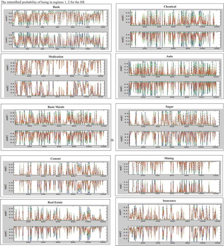For example, in the Investment industry, the duration to stay in regime 1 is 2.7 days and in regime 2 is 3.8 days. The smoothed probability of being in regimes 1 and 2 for each industry are reported in Appendix (B).

According to the smoothed probability, the selected models for each industry suggest that:

• Bank index return started in the turbulent state (regime 2). It continually jumped between the turbulent and calm states until 2016, and often stayed in calm state (regime 1) from 2016 to 2018. Then it jumped between two states from 2018 to 2019 and often stayed in calm state in the last year.

• Auto, Sugar, Real Estate, Cement, Chemical and Basic Metals index returns started in the turbulent state and switched between two states, but they often stayed in turbulent state.

• Medication index return started in the turbulent state and switched between two states, but it often stayed in the calm state.

• Mining and Insurance index returns started in the calm state and switch between two states, but often stayed in calm and turbulent states, respectively.

3.3. Impact of exchange rate on the IIR uncertainty

We also investigate if the exchange rate fluctuations (USD/IRR) impacts the IIR uncertainty. The relationship between the stock prices and exchange rates is well documented in the literature. Currency depreciation can move share prices in either direction. Export-oriented firms which gain international competitiveness and thus export more, are expected to make more profit and enjoy an increase in their share prices. On the other hand, domestic firms that are not export-oriented will face an increase in the cost of imported inputs and perhaps experience a decline in their profit margin and share prices. (Bahmani-Oskooee & Saha, 2016).

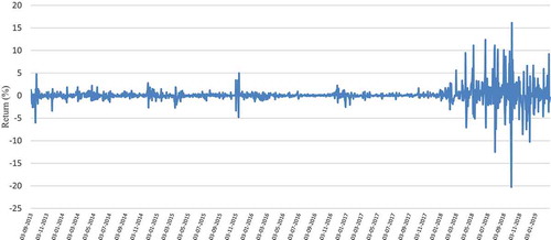
Before estimating the model, we examine the overall trend of the exchange rate in Iran during the period under study. Figures 1 and 2 show the trend of the USD/IRR rate and its fluctuations from 1 September 2013 to 27 February 2019. Between 2013 and 2017 the exchange rate was rising steadily, with some temporary jumps in year ends due to increase in demand. During this period, daily exchange rate fluctuations, except for some periods, were relatively flat and at a maximum of 5%. This relative stability was mainly due to Iran’s active foreign policy that eventually led to a nuclear agreement with 5 + 1 countries (USA, the UK, Russia, Germany, China, and France). Over this period, both international trade, especially oil sales, and foreign domestic investment (FDI) increased which led to reduction in economic uncertainty in Iran. In the beginning of 2018, the political tensions between the new US administration and Iran rose. These tensions, which eventually led to the US government pulling out of the nuclear agreement and imposing economic sanctions against Iran, had a significant impact on the exchange rate with the IRR losing more than 80% of its value over 9 months. Slowing down economic activities which resulted in reduction in imports along with some measures that the Central Bank of Iran undertook, led to a sizable decline in exchange rate towards the end of 2018. However, the exchange rate began rising again in 2019 due to very high inflation and money supply.

Figure 1. The logarithm of the USD/IRR rate from 1 September 2013 to 27 February 2019.

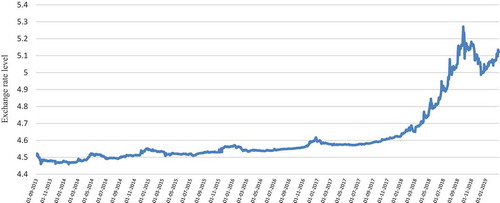
Figure 2. The USD/IRR rate daily returns from 1 September 2013 to 27 February 2019.

In this section, first, we measure the time series of the IIR uncertainty using the optimal model in terms of two different regimes. In order to measure uncertainty, we remove the predictable component of the variation from optimal models by measuring the conditional variance series. After measuring the IIR uncertainty, we estimate the effect of the exchange rate changes on the IIR uncertainty using the ARDL model. The ARDL($p,q$) model specification is given as follows:

(12) $C\left(L,p\right)y_t=\mu +B\left(L,q\right)x_t+u_t$(12)

in which, $y_t$ is time series of uncertainty and $x$ is exchange rate return.⁶ $\mu$ is the vector of other parameters such as the intercept term and time trends. Also, $C\left(L,p\right)=1-{\gamma }_{1}L-{\gamma }_2{L}^2-\dots -{\gamma }_p{L}^p$, and $B\left(L,q\right)={\beta }_0+{\beta }_{1}L+{\beta }_2{L}^2+\dots +{\beta }_q{L}^q$. $L$ is a lag operator. According to ARDL model, long-term effect is given as follows:

(13) $\frac{B\left(L,q\right)}{C\left(L,p\right)}=\frac{{\sum }_{j=0}^q{\beta }_j}{1-{\sum }_{j=1}^p{\gamma }_j}$(13)

The short-term effect is calculated form below equation:

(14) $\mathrm{\Delta }{y}_t={\beta }_0\mathrm{\Delta }{x}_t+a{u}_{t-1}+{\epsilon }_t$(14)

where, ${\beta }_0$ is short-term effect. Also $u_{t-1}=y_{t-1}-\frac{\mu }{1-\left({\gamma }_1+\dots +{\gamma }_p\right)}-\frac{{\beta }_0+{\beta }_1+\dots +{\beta }_q}{1-\left({\gamma }_1+\dots +{\gamma }_p\right)}{x}_{t-1}$

We use SIC to select optimal lags ($p$ and $q$) for modeling relationship between the IIR uncertainty and exchange rate. The detailed results are lengthy and are not reported in the paper. Table 10 shows the final ARDL($p,q$) model with short-term and long-term effects of the exchange rate on the IIR uncertainty under two regimes. Long-term and short-term effects were estimated based on Eq. (13)(13) $\frac{B\left(L,q\right)}{C\left(L,p\right)}=\frac{{\sum }_{j=0}^q{\beta }_j}{1-{\sum }_{j=1}^p{\gamma }_j}$(13) and Eq. (14)(14) $\mathrm{\Delta }{y}_t={\beta }_0\mathrm{\Delta }{x}_t+a{u}_{t-1}+{\epsilon }_t$(14) under final model of ARDL($p,q$). In the first column, the dependent variable is the uncertainty calculated under regime 1, and in the second column, is the uncertainty calculated under regime 2.

Table 10. Short-term and long-term effect of the exchange rate on the IIR uncertainty

Model		Industry	Short- term		Long-term
Regime 1	Regime 2		Regime 1	Regime 2	Regime 1	Regime 2
ARDL(1,1)	ARDL(1,0)	Investment	−0. 5430*** (−5.26)	−0.00002 (−0.68)	−0.00001 (−0.51)	−0.00004 (−0.98)
ARDL(1,2)	ARDL(1,2)	Auto	0. 4870*** (4.56)	0.0261*** (2.65)	0.0105** (2.14)	0.0032** (1.98)
ARDL(0,1)	ARDL(1,0)	Mining	0. 2700*** (3.52)	0.0009 (1.58)	0.0001 (1.48)	0.0007 (1.52)
ARDL(1,1)	ARDL(1,1)	Chemical	0.00132* (1.79)	−0. 4830*** (−4.95)	−0.0004* (−1.65)	0.0018* (1.86)
ARDL(1,0)	ARDL(1,0)	Basic Metals	−0. 0699*** (−2.95)	0. 1090*** (3.62)	−0.0008 (−1.21)	−0.00009 (−0.68)
ARDL(1,2)	ARDL(1,2)	Cement	−0.0430** (−2.31)	−0.0253** (−1.99)	0.0458**- (−2.51)	−0.044** (−2.41)
ARDL(1,1)	ARDL(1,0)	Sugar	−0.0355** (−2.14)	−0.0005 (−1.2)	−0.0094* (−1.74)	−0.0001 (−1.04)
ARDL(1,1)	ARDL(1,0)	Bank	−0.0121** (−2.15)	−0.0006 (−1.12)	−0.0045* (−1.73)	−0.0007 (−1.23)
ARDL(1,2)	ARDL(1,2)	Real Estate	−0.0102* (−1.89)	−0.0116** (−2.05)	−0.0142** (−2.14)	−0.024*** (−2.65)
ARDL(1,1)	ARDL(1,1)	Medication	0.0074* (1.70)	0.0185** (2.41)	0.0479** (2.51)	0.0325** (2.12)
ARDL(1,1)	ARDL(1,1)	Food	−0.0040*** (−2.69)	−0.0033** (−2.45)	−0.0005* (−1.69)	−0.0005* (−1.68)
ARDL(1,2)		Oil Products	−0.037** (−2.14)		−0.0004* (−1.71)
ARDL(1,2)		Rubber	−0.032*** (−3.15)		−0.0003* (−1.81)
ARDL(2,1)	ARDL(1,1)	Machinery	0.036** (2.10)	0.037** (2.15)	0.0003* (1.81)	0.0002* (1.73)
ARDL(1,1)	ARDL(2,1)	Ceramic Tile	−0.032*** (−3.17)	−0.035*** (−3.25)	−0.0013* (−1.84)	−0.0009* (−1.73)
ARDL(1,0)	ARDL(1,0)	Insurance	−0.00005 (−0.89)	−0.00004 (−0.74)	−0.00003 (−0.74)	−0.00001 (−0.24)
ARDL(1,0)		Metal products	−0.00001 (0.98)		(0.00002) (1.12)

Note: * indicates significance at the 10% level; **, at the 5% level; and *** at the 1% level. t-statistics are reported in parentheses.

Most of the estimated parameters are significant at 1%, 5% and 10% levels. In the short-term and long-term, the impact of exchange rate on the return uncertainty of the Insurance and Metal products indexes under two regimes is insignificant. However, exchange rate has a significant impact on the return uncertainty of the Investment, Mining, Sugar, and Bank indexes only under regime 1. Insurance companies are classified in the service sector. Since the service sector in comparison with other economic sectors is rarely related to foreign trade, especially in developing countries (with the exception of the banking sector, which holds foreign exchange reserves and participates in foreign trade as a third party), it is logical that the coefficients of service companies be insignificant. The coefficient of the return uncertainty of the Bank index is significant in regime 1 in both short-term and long-term.

Some industries such as sugar receive large part of their inputs from inside the country and sell their products in domestic markets. Nevertheless, their products are affected by the inflationary effects of exchange rate fluctuations. In addition to being active mainly in domestic markets, some industries such as Metal products and Mining are protected by government against some systematic risks such as exchange rate shocks. Therefore, exchange rate has less effect on their return uncertainty.

When the exchange rate increases, in the short-term the Investment industry index return uncertainty decreases under regime 1, but in the long term, its effect is not significant. The exchange rate fluctuations have a significant effect on the return uncertainty of other industry indices under two regimes in the short-term and long-term. Among these industries, some such as Auto, Medication and Machinery are heavily dependent on import. Moreover, some industries such as Chemical, Basic metals, and Oil products export more than half of their products to other countries. Thus, as we expect, the coefficients of the above two groups are significant.

The results of ARDL model show that the exchange rate has a negative effect on export-oriented industries’ uncertainty, i.e., increase in exchange rate reduces return uncertainty and vice versa. This is expected because export-oriented industries benefit from higher exchange rates. Reduction in exchange rates, on the other hand, imposes some uncertainty due to unexpected interventions of large (mostly government-sponsored) investment firms that try to keep the value of these companies. The same logic, with opposite effects, applies to import-oriented industries which explains the results of ARDL model.

We can interpret the overall results of Table 10 in another aspect. According to Table 10, in many industries, exchange rate appreciation reduces the IIR uncertainty. These results can be interpreted using the concept of uncertainty. As mentioned in the Introduction Section, the uncertainty is an unpredictable component of any time series. In the Iranian economy, high growth in money supply over the past years (for instance, between 2013 and 2019 the money supply on average grew 27% per year) has been the main economic driver of rising inflation and devaluation of the national currency. This phenomenon is not unknown to and unpredictable by investors, and hence, is reflected into stock prices without having a huge impact on the unpredictable component. In contrast, when the exchange rate falls temporarily, contrary to investors’ expectations, the unpredictable component (or forecast error) increases, so does the uncertainty. Therefore, the negative relationship between the exchange rate and the uncertainty is justified for many industries.

4. Conclusion

The goal of this study is to measure the IIR uncertainty by improving models of MRS-GARCH family and to estimate the impact of changes in exchange rate on the IIR uncertainty. We first apply MRS-GARCH family models to estimate the IIR volatility. Then, we compare their performances with those of ARMA-GARCH family models under the normal, Student’s-t and GED distributions. We find that MRS-GARCH models are more powerful to model the IIR volatility. This indicates that a switching behaviour exists in the IIR indexes. We also show that MRS-EGARCH-M models under GED and Student’s t-distributions outperform other MRS-GARCH models.

We estimate the impact of the exchange rate on the IIR uncertainty in a regime-switching environment. The results show that the exchange rate has a negative and positive impact on the IIR uncertainty for export and import-oriented companies, respectively, under both regimes.

Our findings have several economic and financial implications. Knowing the stock prices trend under different regimes (and their transition probabilities between regimes) helps investors to predict the stock prices more accurately. Moreover, having a better understanding of uncertainty and its magnitude enables investors to measure the risk.

There are several avenues to extend this research. First, one could investigate the performances of MRS-GARCH models for forecasting and calculating value at risk (VaR). Second, since volatility is a key input in option pricing formulas, it would be interesting to compare the performances of MRS-GARCH models and other popular models to price options. Third, the univariate MRS-GARCH models could be extended to multivariate ones, which could model the covariance between two different asset returns in order to estimate hedging and asset allocation.

Additional information

Funding

The authors received no direct funding for this research.

Notes on contributors

Mehdi Zolfaghari

Mehdi Zolfaghari is Assistant Professor in Economics department, Tarbiat Modares University, Tehran, Iran. He obtained his Ph.D. degree (Financial Economics) from Tarbiat Modares University. He has published a number of articles ranging from financial economics to energy economics. His current area of research is financial economics.

Saeid Hoseinzade

Saeid Hoseinzade is Assistant Professor of finance in Suffolk University, Boston, USA. He obtained his Ph.D. degree (Finance) from Boston College. He has a strong interest in measuring risk and uncertainty in financial markets. He is also working on a project that studies new models to measure risk and uncertainty.

Notes

1. MRS-GARCH family models include MRS-GARCH, MRS-GARCH-M, MRS-EGARCH, MRS-EGARCH-M, MRS-IGARCH, and MRS-IGARCH-M.

2. ARMA-GARCH family models including ARMA-GARCH, ARMA -GARCH-M, ARMA -EGARCH, ARMA -EGARCH-M, ARMA-IGARCH, and ARMA -IGARCH-M.

3. The ARIMA(p, d, q) process of autoregressive order “p” and moving average order “q” and integration order “d” can be described as:

$x_t=c+\sum _{i=1}^p{\alpha }_i{x}_{t-i}+\sum _{j=1}^q{\beta }_j{\epsilon }_{t-j}+\epsilon$

4. $\rho$ and $q$ are probabilities of the volatility remaining in the same regime.

5. There are usually two exchange rates in Iran, the official and the unofficial exchange rate. In recent years, the official exchange rate, which has been almost constant, has been used by the government to import vital goods (such as wheat, corn and medicine). But the unofficial exchange rate (which is partly controlled by the central bank) accounts for a significant portion of the country’s currency market. Private sector exporters and importers use this rate to convert domestic currency into foreign (and vice versa) through currency exchanges. For this reason, unofficial exchange rate changes are used as an exogenous variable affecting stock prices, inflation rate, etc. in most economic studies (e.g., Abounoori & Tour, 2019; Davoudi et al., 2018; Zolfaghari & Sahabi, 2017). Following the literature and given that the official exchange rates’ fluctuation is almost non-existent, we use unofficial exchange rate in this study. Due to the facility of buying and selling foreign currency by individuals and companies, there is no black market in this regard. However, some government agencies (such as the Center for Combating Smuggling of Goods and Foreign Currency) monitor indirectly the very large and suspicious transactions.

6. Iran has a high inflation and high interest rates compared to the US which affects the exchange rates in medium-term and long-term. Since our analysis is daily, the impact of inflation/interest rates differential on the exchange rate is negligible. Therefore, daily exchange rate returns are not adjusted for inflation/interest rates.

 

Appendix (A)

The conditional mean and variance models under Markov-switching

The conditional mean and variance models for the Chemical industry under Markov-switching

Table

Model	Type	Distribution	${\mu }_1$	${\mu }_2$	${\lambda }_1$	${\lambda }_2$	$b_{01}$	$b_{02}$
GARCH	simple	Normal	0.367	−0.08			1.959	0.023
		t	0.509	−0.04			0.078	0.13
		GED	−0.03	0.887			0.049	1.697
	In-mean	Normal	−6.49	−6.89	4.918	13.64	1.955	0
		t	0.055	0.011	−0.082	0.568	0	0.053
		GED	−2.06	0.003	2.097	−0.151	0.762	0.011
EGARCH	simple	Normal	1.47	−0.02			0.762	−0.808
		t	1.339	−0.08			0.123	−0.265
		GED	1.471	−0.02			0.762	−0.808
	In-mean	Normal	−0.34	−12.5	1.417	9.738	−0.96	0.534
		t	−12.1	1.642	10.295	−1.454	0.35	0.23
		GED	1.174	−2.24	−2.009	3.323	−0.405	−0.29
IGARCH	simple	Normal	2.321	7.096			0.963	0.002
		t	0.631	0.269			0.125	0.159
		GED	−0.96	0.263			0.023	0.098
	In-mean	Normal	6.388	6.034	−4.185	−6.806	1.961	0.001
		t	0.53	0.133	0.002	−0.4	0.089	0.117
		GED	−0.11	0.104	1.08	−0.289	0.006	0.047
Model	$b_{11}$	$b_{12}$	$b_{21}$	$b_{22}$	$b_{31}$	$b_{32}$	$p_{11}$	$p_{22}$
GARCH	0.001	0.222	0.001	0.118			0.76	0.86
	0	0.934	0.998	0.066			0.68	0.85
	0.602	0.022	0.351	0.015			0.64	0.85
	0.011	0	0	0.093			0.78	0.91
	0.058	0.008	0.942	0.992			0.87	0.91
	0.018	0.504	0.603	0.179			0.76	0.9
EGARCH	−0.14	0.508	−0.319	−0.055	0.03	0.985	0.67	0.93
	0.447	0.651	−0.087	−0.2	0.984	0.982	0.68	0.93
	−0.14	0.508	−0.319	−0.055	0.03	0.983	0.67	0.93
	−0.97	0.01	0.987	0.058	0.569	0.026	0.81	0.85
	0.01	−0.215	0.064	−0.298	0.031	0.223	0.93	0.91
	0.328	0.119	−0.322	0.271	0.864	0.584	0.64	0.74
IGARCH	0.932	0.745	0.068	0.255			0.85	0.79
	0.025	0.963	0.975	0.037			0.84	0.79
	0.868	0.096	0.132	0.904			0.87	0.78
	0.963	0.88	0.037	0.12			0.87	0.75
	0.015	0.993	0.985	0.007			0.87	0.78
	0.937	0.021	0.063	0.979			0.86	0.79

The conditional mean and variance models for the Bank industry under Markov-switching

Table

Model	Type	Distribution	${\mu }_1$	${\mu }_2$	${\lambda }_1$	${\lambda }_2$	$b_{01}$	$b_{02}$	$b_{11}$
GARCH	simple	Normal	−0.120	0.305			0.052	0.341	0.229
		t	−0.151	0.459			0.050	0.025	0.668
		GED	−0.133	0.418			0.097	0.015	0.554
	In-mean	Normal	−0.363	−0.842	0.594	3.790	1.614	0.002	0.504
		t	−0.012	−0.015	−0.291	0.725	0.052	0.135	0.599
		GED	0.038	−0.054	−0.414	0.798	0.053	0.161	0.475
EGARCH	simple	Normal	−0.037	0.380			−1.000	0.845	0.409
		t	−0.139	0.598			0.98-	−0.207	0.644
		GED	−0.129	0.679			0.98-	−0.236	0.571
	In-mean	Normal	1.053	1.122	−2.548	−0.491	0.98-	−0.113	−0.090
		t	0.053	−2.904	−0.245	3.911	−0.289	−0.120	0.191
		GED	0.963	1.505	−0.358	−3.041	−0.135	−0.811	0.259
IGARCH	simple	Normal	−0.325	0.756			0.963	0.024	0.493
		t	−0.010	−0.036			0.063	0.156	0.520
		GED	0.186	0.065			0.124	0.032	0.474
	In-mean	Normal	−0.399	−0.866	0.616	3.776	1.601	0.001	0.527
		t	−0.012	−0.015	−0.291	0.725	0.052	0.135	0.599
		GED	0.119	0.011	0.527	−0.324	0.096	0.053	0.393
Model	$b_{12}$	$b_{21}$	$b_{22}$	$b_{31}$	$b_{32}$	$p_{11}$	$p_{22}$
GARCH	0.249	0.117	0.608			0.74	0.79
	0.102	0.332	0.898			0.75	0.78
	0.095	0.283	0.905			0.74	0.78
	0.323	0.496	0.448			0.81	0.83
	0.434	0.401	0.566			0.82	0.83
	0.293	0.318	0.549			0.81	0.82
EGARCH	0.057	0.112	−0.115	0.990	0.990	0.82	0.8
	0.548	0.003	−0.208	0.985	0.990	0.87	0.78
	0.523	−0.023	−0.205	0.984	0.990	0.87	0.77
	0.252	−0.680	−0.023	0.342	0.753	0.94	0.93
	−0.126	−0.005	0.471	0.981	0.603	0.77	0.71
	0.146	−0.015	−0.446	0.759	0.424	0.95	0.96
IGARCH	0.544	0.508	0.456			0.96	0.85
	0.453	0.480	0.547			0.98	0.84
	0.694	0.526	0.306			0.95	0.81
	0.546	0.473	0.454			0.92	0.91
	0.434	0.401	0.566			0.92	0.90
	0.689	0.607	0.311			0.91	0.89

The conditional mean and variance models for the Medication industry under Markov-switching

Table

Model	Type	Distribution	${\mu }_1$	${\mu }_2$	${\lambda }_1$	${\lambda }_2$	$b_{01}$	$b_{02}$
GARCH	simple	Normal	−0.010	0.619			0.010	0.481
		t	−0.039	0.387			0.002	0.002
		GED	−0.029	0.482			0.006	0.229
	In-mean	Normal	−0.097	0.309	0.464	−2.008	0.002	0.282
		t	−0.237	−0.029	1.133	−0.015	0.022	0.001
		GED	−0.237	−0.059	1.324	0.034	0.017	0.008
EGARCH	simple	Normal	−0.021	0.513			−0.980	0.026
		t	−0.035	0.446			−0.138	−0.019
		GED	−0.037	0.407			−0.411	−0.263
	In-mean	Normal	−2.718	−0.253	3.466	1.122	−0.208	−0.178
		t	0.005	−0.667	−0.124	1.863	−0.070	0.080
		GED	−0.020	−1.957	−0.008	3.864	−0.454	−0.057
IGARCH	simple	Normal	−0.120	0.365			0.125	0.363
		t	−0.370	−0.069			0.213	0.126
		GED	0.064	0.013			0.215	0.050
	In-mean	Normal	−0.097	0.309	0.464	−2.008	0.002	0.282
		t	−0.316	−0.029	1.160	−0.015	0.031	0.000
		GED	−0.020	0.066	−0.060	0.725	0.008	0.088
Model	$b_{11}$	$b_{12}$	$b_{21}$	$b_{22}$	$b_{31}$	$b_{32}$	$p_{11}$	$p_{22}$
GARCH	0.412	0.438	0.410	0.094			0.91	0.92
	0.002	0.111	0.975	0.900			0.90	0.91
	0.447	0.620	0.532	0.010			0.80	0.90
	0.746	0.008	0.254	0.973			0.91	0.89
	0.107	0.006	0.894	0.963			0.91	0.87
	0.085	0.216	0.876	0.698			0.89	0.86
EGARCH	0.178	0.104	−0.393	0.035	0.986	0.510	0.93	0.76
	0.334	−0.057	−0.225	0.658	0.990	0.982	0.97	0.93
	0.346	0.216	−0.078	0.134	0.979	0.990	0.97	0.93
	0.053	−0.972	0.301	0.924	0.117	0.967	0.88	0.93
	0.049	−0.370	−0.145	0.426	0.990	0.898	0.94	0.86
	0.458	−0.365	−0.342	0.599	0.908	0.604	0.94	0.83
IGARCH	0.693	0.064	0.307	0.936			0.85	0.81
	0.160	0.130	0.840	0.870			0.84	0.84
	0.415	0.845	0.585	0.155			0.84	0.83
	0.746	0.021	0.254	0.979			0.82	0.80
	0.109	0.044	0.891	0.956			0.81	0.79
	0.382	0.673	0.618	0.327			0.82	0.74

The conditional mean and variance models for the Auto industry under Markov-switching

Table

Model	Type	Distribution	${\mu }_1$	${\mu }_2$	${\lambda }_1$	${\lambda }_2$	$b_{01}$	$b_{02}$	$b_{11}$
GARCH	simple	Normal	1.177	−0.338			3.348	0.102	0.007
		t	2.029	−0.394			0.943	0.148	0.029
		GED	−0.419	1.568			0.232	0.005	0.278
	In-mean	Normal	−0.498	−4.534	2.711	1.785	2.042	0.002	0.001
		t	−0.240	0.024	2.387	−0.412	0.321	0.098	0.087
		GED	−9.268	−0.057	2.518	−0.255	0.707	0.064	0.021
EGARCH	simple	Normal	1.984	−0.380			0.818	−0.772	0.298
		t	2.094	−0.371			−0.991	−0.493	−0.264
		GED	2.151	−0.371			0.473	−0.663	−0.262
	In-mean	Normal	21.051	−3.045	−10.734	3.273	1.337	−0.330	−0.008
		t	−5.663	1.551	4.948	−1.897	0.140	−0.169	0.091
		GED	0.873	−5.718	−0.378	4.459	0.157	0.333	0.007
IGARCH	simple	Normal	−1.986	−1.326			2.146	0.037	0.692
		t	0.964	0.370			0.127	0.636	0.397
		GED	1.026	−0.563			0.013	0.139	0.414
	In-mean	Normal	−2.714	−6.949	3.442	4.052	3.171	0.002	0.767
		t	0.283	0.620	−0.479	0.592	0.315	0.100	0.328
		GED	1.006	−0.127	0.408	−0.238	0.000	0.208	0.375
Model	$b_{12}$	$b_{21}$	$b_{22}$	$b_{31}$	$b_{32}$	$p_{11}$	$p_{22}$
GARCH	0.239	0.008	0.605			0.75	0.81
	0.267	0.016	0.621			0.74	0.85
	0.079	0.521	0.779			0.74	0.81
	0.037	0.224	0.986			0.71	0.86
	0.207	0.150	0.685			0.75	0.87
	0.176	0.016	0.765			0.75	0.85
EGARCH	0.411	−0.553	0.004	0.099	0.970	0.66	0.91
	0.325	0.116	−0.007	0.978	0.985	0.65	0.93
	0.384	−0.001	−0.054	0.036	0.987	0.65	0.91
	0.067	−0.031	0.297	0.000	0.060	0.98	0.97
	0.123	0.098	−0.215	0.542	0.713	0.69	0.76
	0.098	−0.005	0.172	0.886	0.140	0.91	0.93
IGARCH	0.037	0.308	0.963			0.69	0.71
	0.964	0.604	0.037			0.63	0.71
	0.616	0.586	0.384			0.62	0.69
	0.026	0.233	0.974			0.68	0.84
	0.322	0.672	0.678			0.69	0.85
	0.538	0.625	0.462			0.68	0.71

The conditional mean and variance models for the Basic metals industry under Markov-switching

Table

Model	Type	Distribution	${\mu }_1$	${\mu }_2$	${\lambda }_1$	${\lambda }_2$	$b_{01}$	$b_{02}$
GARCH	simple	Normal	−0.120	0.337			0.243	2.013
		t	−0.143	1.077			0.055	0.073
		GED	−0.137	1.319			0.049	1.525
	In-mean	Normal	−0.358	−0.078	0.614	0.964	0.005	0.153
		t	−0.327	−0.225	1.088	−0.018	0.002	0.021
		GED	−7.780	−0.179	3.580	0.003	0.987	0.028
EGARCH	simple	Normal	0.493	−0.126			0.728	−1.366
		t	1.140	−0.145			−0.007	−0.562
		GED	1.062	−0.154			−0.025	−0.538
	In-mean	Normal	17.505	1.329	−12.466	−2.829	0.647	−1.000
		t	−11.467	2.937	8.394	−6.039	0.668	−1.000
		GED	15.702	−3.471	−11.417	5.460	0.599	−0.993
IGARCH	simple	Normal	0.986	1.799			0.365	0.360
		t	−0.326	−0.856			0.126	0.963
		GED	−0.126	−0.365			0.452	0.215
	In-mean	Normal	1.132	1.696	−2.397	1.814	0.257	2.088
		t	−0.501	−0.206	1.051	−0.030	0.102	0.008
		GED	−0.282	−0.221	1.045	0.041	0.043	0.041
Model	$b_{11}$	$b_{12}$	$b_{21}$	$b_{22}$	$b_{31}$	$b_{32}$	$p_{11}$	$p_{22}$
GARCH	0.053	0.078	0.012	0.096			0.75	0.84
	0.227	0.052	0.660	0.948			0.78	0.70
	0.206	0.023	0.671	0.024			0.74	0.69
	0.010	0.013	0.181	0.986			0.78	0.74
	0.129	0.076	0.871	0.798			0.78	0.74
	0.024	0.193	0.239	0.638			0.77	0.75
EGARCH	0.041	0.039	−0.074	−0.178	0.145	0.533	0.92	0.93
	0.233	0.276	−0.117	−0.143	0.988	0.989	0.76	0.92
	0.196	0.260	−0.104	−0.114	0.979	0.991	0.76	0.92
	−0.004	0.096	−0.037	−0.409	0.013	0.307	0.96	0.94
	0.004	−0.050	0.057	−0.149	0.096	0.245	0.97	0.96
	−0.002	−0.031	−0.042	0.137	0.002	0.096	0.97	0.96
IGARCH	0.214	0.963	0.786	0.037			0.92	0.78
	0.854	0.256	0.146	0.744			0.92	0.63
	0.370	0.457	0.630	0.543			0.91	0.85
	0.984	0.955	0.016	0.046			0.89	0.56
	0.184	0.177	0.816	0.823			0.89	0.88
	0.293	0.330	0.707	0.670			0.88	0.89

The conditional mean and variance models for the Sugar industry under Markov-switching

Table

Model	Type	Distribution	${\mu }_1$	${\mu }_2$	${\lambda }_1$	${\lambda }_2$	$b_{01}$	$b_{02}$
GARCH	simple	Normal	1.443	0.009			5.538	0.009
		t	1.676	−0.043			1.876	0.013
		GED	−0.035	1.745			0.019	2.636
	In-mean	Normal	−0.073	0.996	0.178	−4.303	0.963	3.112
		t	0.202	0.175	0.944	−0.412	0.158	0.037
		GED	−3.876	0.130	3.697	−0.375	1.287	0.027
EGARCH	simple	Normal	0.922	0.122			2.000	−0.711
		t	−0.070	1.169			−0.120	0.036
		GED	1.701	−0.056			0.955	−0.909
	In-mean	Normal	2.801	0.085	−0.689	−0.206	1.485	−0.518
		t	0.384	0.316	−0.105	0.174	0.020	0.124
		GED	−1.261	−8.372	1.545	5.451	−0.072	0.749
IGARCH	simple	Normal	−0.962	0.963			0.211	1.524
		t	−0.124	0.893			0.045	0.652
		GED	0.635	0.962			0.313	0.741
	In-mean	Normal	−0.075	1.000	0.181	−4.293	0.005	3.122
		t	0.135	0.564	0.359	−0.203	0.381	0.002
		GED	−0.238	0.197	0.987	−0.459	0.041	0.132
Model	$b_{11}$	$b_{12}$	$b_{21}$	$b_{22}$	$b_{31}$	$b_{32}$	$p_{11}$	$p_{22}$
GARCH	0.007	0.324	0.037	0.563			0.90	0.91
	0.018	0.381	0.215	0.619			0.90	0.89
	0.420	0.007	0.576	0.636			0.89	0.89
	0.037	0.214	0.149	1.000			0.85	0.91
	0.178	0.384	0.653	0.616			0.84	0.89
	0.026	0.518	0.321	0.482			0.79	0.87
EGARCH	0.483	0.174	−0.020	0.020	0.970	0.957	0.94	0.95
	0.549	0.894	−0.362	−0.555	0.937	0.987	0.95	0.85
	0.262	0.560	−0.237	−0.174	0.024	0.957	0.78	0.95
	−0.405	0.227	−0.336	−0.167	0.372	0.937	0.71	0.9
	0.026	0.053	−0.023	−0.011	0.985	0.962	0.99	0.99
	−0.128	0.054	0.391	0.111	0.729	0.008	0.92	0.78
IGARCH	0.632	0.692	0.368	0.308			0.90	0.80
	0.425	0.057	0.575	0.943			0.90	0.81
	0.042	0.326	0.958	0.674			0.89	0.74
	0.850	0.562	0.150	0.438			0.89	0.69
	0.365	0.017	0.635	0.983			0.88	0.74
	0.065	0.661	0.936	0.339			0.84	0.85

The conditional mean and variance models for the Cement industry under Markov-switching

Table

Model	Type	Distribution	${\mu }_1$	${\mu }_2$	${\lambda }_1$	${\lambda }_2$	$b_{01}$	$b_{02}$	$b_{11}$
GARCH	simple	Normal	−0.093	0.243			0.036	0.128	0.185
		t	0.671	−0.086			0.031	0.012	0.154
		GED	−0.080	0.785			0.013	0.017	0.259
	In-mean	Normal	−0.151	0.164	0.292	−1.358	0.006	0.124	0.002
		t	0.039	−0.269	−0.391	1.296	0.032	0.064	0.460
		GED	−0.169	0.044	1.326	−0.449	0.035	0.027	0.156
EGARCH	simple	Normal	0.619	−0.086			−0.205	−0.802	0.385
		t	0.588	−0.087			−0.194	−0.613	0.430
		GED	0.922	−0.071			−0.287	−0.706	0.298
	In-mean	Normal	−3.028	−0.817	3.081	2.463	0.168	−0.118	−0.034
		t	−0.066	0.074	1.152	−0.399	0.196	−0.263	−0.335
		GED	−4.240	−0.886	3.950	2.056	0.253	−0.199	0.014
IGARCH	simple	Normal	0.213	0.452			0.057	0.147	0.462
		t	0.456	0.713			0.366	0.237	0.368
		GED	−0.144	0.345			0.068	0.216	0.164
	In-mean	Normal	−0.164	0.221	0.300	−1.398	0.014	0.112	0.547
		t	0.245	0.678	0.462	−0.345	0.407	0.210	0.325
		GED	−0.093	0.243	0.257	−0.396	0.036	0.128	0.185
Model	$b_{12}$	$b_{21}$	$b_{22}$	$b_{31}$	$b_{32}$	$p_{11}$	$p_{22}$
GARCH	0.154	0.084	0.788			0.82	81
	0.274	0.846	0.623			0.81	0.90
	0.140	0.606	0.860			0.76	0.91
	0.097	0.386	0.985			0.90	0.89
	0.220	0.447	0.780			0.087	0.88
	0.339	0.795	0.403			0.87	0.88
EGARCH	0.527	−0.120	−0.031	0.978	0.990	0.81	0.93
	0.559	−0.103	0.036	0.986	0.975	0.85	0.95
	0.556	−0.099	0.046	0.990	0.957	0.83	0.96
	−1.046	0.263	1.080	0.064	0.932	0.91	0.95
	0.224	0.366	−0.391	0.893	0.907	0.77	0.93
	−0.232	0.208	0.873	0.065	0.918	0.98	0.99
IGARCH	0.068	0.538	0.932			0.91	0.82
	0.057	0.633	0.943			0.92	0.87
	0.029	0.836	0.971			0.87	0.75
	0.057	0.453	0.943			0.85	0.80
	0.046	0.676	0.954			0.88	0.74
	0.154	0.815	0.846			0.83	0.83

The conditional mean and variance models for the Mining industry under Markov-switching

Table

Model	Type	Distribution	${\mu }_1$	${\mu }_2$	${\lambda }_1$	${\lambda }_2$	$b_{01}$	$b_{02}$	$b_{11}$
GARCH	simple	Normal	−0.037	0.747			0.001	4.411	0.279
		t	−0.030	2.269			0.001	2.393	0.333
		GED	−0.035	2.103			0.002	2.742	0.316
	In-mean	Normal	−0.039	0.426	0.025	−0.199	0.016	4.397	0.409
		t	0.004	−7.384	−0.147	4.627	0.025	2.432	0.448
		GED	−15.236	−0.005	7.299	−0.145	2.694	0.001	0.003
EGARCH	simple	Normal	0.950	−0.095			1.668	−0.987	−0.107
		t	−0.063	2.367			−0.462	1.995	1.364
		GED	−0.064	2.055			−0.757	0.919	0.626
	In-mean	Normal	0.002	5.534	−0.109	−2.724	−0.664	1.441	0.192
		t	−11.582	0.038	6.856	−0.266	0.958	−0.592	0.060
		GED	0.010	−8.418	−0.172	5.550	−0.705	0.712	0.325
IGARCH	simple	Normal	−0.126	0.524			0.013	5.370	0.512
		t	0.513	−0.124			0.216	0.064	0.416
		GED	0.163	−0.096			0.053	0.962	0.496
	In-mean	Normal	−0.039	0.426	0.025	−0.199	0.005	4.397	0.409
		t	−0.413	−0.075	0.100	0.641	0.155	0.004	0.472
		GED	0.014	−0.049	−0.216	0.483	0.002	1.854	0.459
Model	$b_{12}$	$b_{21}$	$b_{22}$	$b_{31}$	$b_{32}$	$p_{11}$	$p_{22}$
GARCH	0.025	0.504	0.085			0.88	0.80
	0.043	0.667	0.096			0.92	0.75
	0.030	0.680	0.076			0.94	0.91
	0.988	0.591	0.000			0.94	0.91
	0.042	0.552	0.375			0.93	0.86
	0.389	0.182	0.543			0.95	0.98
EGARCH	0.308	−0.090	−0.098	0.006	0.914	0.8	0.95
	0.321	−0.461	0.110	0.985	0.128	0.97	0.76
	0.064	−0.159	0.007	0.925	0.030	0.97	0.78
	−0.236	−0.257	−0.237	0.932	0.002	0.87	0.74
	0.235	0.072	−0.307	0.102	0.977	0.78	0.8
	0.088	−0.191	0.112	0.973	0.056	0.84	0.84
IGARCH	0.936	0.488	0.064			0.92	0.78
	0.635	0.584	0.365			0.91	0.85
	0.895	0.504	0.105			0.93	0.89
	0.933	0.591	0.067			0.85	0.79
	0.484	0.528	0.516			0.84	0.8
	0.936	0.541	0.064			0.79	0.87

The conditional mean and variance models for the Real Estate industry under Markov-switching

Table

Model	Type	Distribution	${\mu }_1$	${\mu }_2$	${\lambda }_1$	${\lambda }_2$	$b_{01}$	$b_{02}$
GARCH	simple	Normal	0.734	−0.065			0.037	0.001
		t	0.935	−0.051			0.023	0.006
		GED	−0.030	1.204			0.013	0.000
	In-mean	Normal	−0.111	0.227	0.164	1.044	0.010	0.008
		t	−0.522	0.073	1.811	−0.275	0.208	0.000
		GED	0.128	−1.193	−0.378	2.387	0.002	0.301
EGARCH	simple	Normal	0.347	−0.055			0.200	0.463
		t	0.966	−0.058			0.510	0.500
		GED	1.176	−0.038			0.409	0.470
	In-mean	Normal	2.752	−1.341	−2.814	2.908	0.077	−0.279
		t	−1.208	0.332	2.365	−0.764	−0.288	−0.175
		GED	−3.679	−1.485	13.663	2.465	0.712	−0.666
IGARCH	simple	Normal	−0.035	0.299			0.130	0.235
		t	0.213	0.135			0.046	0.138
		GED	0.099	0.090			0.095	0.024
	In-mean	Normal	−0.087	0.272	0.099	−1.306	0.010	0.163
		t	−0.155	0.077	1.033	−0.274	0.075	0.005
		GED	−0.010	0.070	0.877	−0.243	0.043	0.007
Model	$b_{11}$	$b_{12}$	$b_{21}$	$b_{22}$	$b_{31}$	$b_{32}$	$p_{11}$	$p_{22}$
GARCH	0.024	0.258	0.976	0.678			0.82	0.81
	0.061	0.263	0.923	0.679			0.84	0.83
	0.203	0.036	0.743	0.937			0.86	0.89
	0.000	0.000	0.511	1.000
	0.250	0.215	0.308	0.783			0.87	0.91
	0.150	0.236	0.816	0.211			0.79	0.8
EGARCH	−0.075	0.015	0.987	0.992	0.520	0.800	0.78	0.74
	−0.292	−0.075	0.977	0.990	0.730	0.949	0.91	0.72
	−0.215	−0.073	0.987	0.977	0.722	0.966	0.87	0.76
	−0.102	−0.175	−0.247	0.500	0.751	0.966	0.82	0.84
	0.213	0.045	0.281	−0.224	0.639	0.934	0.71	0.87
	0.017	0.153	0.038	0.402	0.053	0.404	0.98	0.99
IGARCH	0.398	0.077	0.602	0.923			0.91	0.83
	0.543	0.125	0.457	0.876			0.92	0.81
	0.623	0.258	0.377	0.742			0.86	0.85
	0.488	0.049	0.512	0.952			0.94	0.79
	0.425	0.177	0.575	0.823			0.97	0.87
	0.431	0.239	0.569	0.761			0.87	0.76

The conditional mean and variance models for the Insurance industry under Markov-switching

Table

Model	Type	Distribution	${\mu }_1$	${\mu }_2$	${\lambda }_1$	${\lambda }_2$	$b_{01}$	$b_{02}$	$b_{11}$
GARCH	simple	Normal	0.014	−0.049			−0.216	0.483	0.005
		t	−0.007	−0.018			0.003	0.162	0.822
		GED	−0.019	−0.001			0.176	0.002	0.009
	In-mean	Normal	−0.696	0.126	0.927	−0.510	0.273	0.007	0.079
		t	0.126	−0.705	−0.51	0.929	0.007	0.275	0.675
		GED	−0.494	0.141	1.125	−0.380	0.136	0.065	0.646
EGARCH	simple	Normal	0.018	−0.086			−1.000	1.709	0.385
		t	1.088	−0.047			−0.083	−0.304	0.511
		GED	−0.026	1.152			−0.300	−0.201	0.303
	In-mean	Normal	0.019	−0.209	−0.02	0.149	−0.904	2.000	0.045
		t	−2.027	0.309	2.413	−0.620	−0.101	−0.172	0.174
		GED	−2.243	0.323	2.756	−0.630	−0.140	−0.184	0.141
IGARCH	simple	Normal	−0.143	−0.503			1.987	0.056	0.032
		t	0.098	−0.345			0.045	0.780	0.076
		GED	0.143	0.098			0.057	0.345	0.087
	In-mean	Normal	−0.072	−0.202	0.095	5.723	3.141	0.012	0.089
		t	0.128	−0.621	−0.560	0.825	0.009	0.230	0.688
		GED	−0.022	0.061	1.016	−0.290	0.013	0.008	0.891
Model	$b_{12}$	$b_{21}$	$b_{22}$	$b_{31}$	$b_{32}$	$p_{11}$	$p_{22}$
GARCH	1.854	0.459	0.936			0.82	0.88
	0.037	0.178	1.000			0.74	0.76
	0.739	0.996	0.261			0.83	0.82
	0.672	0.952	0.322			0.82	0.79
	0.089	0.325	0.952			0.82	78
	0.113	0.295	0.942			0.83	0.8
EGARCH	0.468	0.106	−0.056	0.980	0.951	0.93	0.94
	0.502	−0.047	0.063	0.982	0.987	0.85	0.969
	0.324	0.049	−0.125	0.965	0.970	0.98	0.888
	−0.051	0.079	−0.063	0.967	0.925	0.82	0.086
	0.086	0.260	−0.116	0.565	0.923	0.79	0.85
	0.071	0.274	−0.132	0.577	0.912	0.77	0.82
IGARCH	0.856	0.968	0.144			0.78	0.86
	0.015	0.924	0.985			0.74	0.72
	0.234	0.913	0.766			0.68	0.81
	0.757	0.911	0.243			0.78	0.86
	0.087	0.312	0.913			0.74	0.72
	0.101	0.109	0.899			0.68	0.81

 

Appendix (B)

The smoothed probability of being in regimes 1, 2 for the IIR

References

- Abounoori, E., Elmi, Z., & Nademic, Y. (2016). Forecasting Tehran stock exchange volatility; Markov switching GARCH approach. Physica A, 445, 264–49. https://doi.org/10.1016/j.physa.2015.10.024
- Abounoori, E., & Tour, M. (2019). Stock market interactions among Iran, USA, Turkey, and UAE. Physica A: Statistical Mechanics and Its Applications, 524, 297–305. https://doi.org/10.1016/j.physa.2019.04.232
- Abouwafia, H. E., & Chambers, M. J. (2015). Monetary policy, exchange rates and stock prices in the Middle East region. International Review of Financial Analysis, 37, 14–28. https://doi.org/10.1016/j.irfa.2014.11.001
- Alsalman, Z. (2016). Oil price uncertainty and the U.S. stock market analysis based on a GARCH-in-mean VAR model. Energy Economics, 59, 251–260. https://doi.org/10.1016/j.eneco.2016.08.015
- Bahmani-Oskooee, M., & Saha, S. (2016). Do exchange rate changes have symmetric or asymmetric effects on stock prices? Global Finance Journal, 31, 57–72. https://doi.org/10.1016/j.gfj.2016.06.005
- Birtoiu, A., & Dragu, F. (2012). The performance of time-varying volatility and regime switching models in estimating Value-at-Risk. Master Thesis. Lund University School of Economics and Management
- Bollerslev, T. (1986). Generalized Autoregressive Conditional Heteroscedasticity. Journal of Econometrics, 31(3), 307–327. https://doi.org/10.1016/0304-4076(86)90063-1
- Box, G. E. P., & Jenkins, G. (1970). Time series analysis, forecasting and control. Holden Day San Francisco.
- Buth, B., Kakinaka, M., & Miyamoto, H. (2015). Inflation and inflation uncertainty: The case of Cambodia, Lao PDR, and Vietnam. Journal of Asian Economics, 38, 31–43. https://doi.org/10.1016/j.asieco.2015.03.004
- Cai, J. (1994). A markov model of switching-regime arch. Business Economic, 12, 309–316.
- Caporale, G. M., Alia, F. M., & Spagnolo, N. (2015). Exchange rate uncertainty and international portfolio flows: A multivariate GARCH-in-mean approach. Journal of International Money and Finance, 54, 70–92. https://doi.org/10.1016/j.jimonfin.2015.02.020
- Chuliá, H., Guillén, M., & Uribe, J. (2017). Measuring uncertainty in the stock market. International Review of Economics and Finance, 48, 18–33. https://doi.org/10.1016/j.iref.2016.11.003
- Conrad, C., & Hartmann, M. (2019). On the determinants of long-run inflation uncertainty: Evidence from a panel of 17 developed economies. European Journal of Political Economy, 56, 233–250. https://doi.org/10.1016/j.ejpoleco.2018.09.002
- Daniela, Z., Mihail-Ioana, C., & Sorinaa, P. (2014). Inflation uncertainty and inflation in the case of Romania, Czech Republic, Hungary, Poland and Turkey. Procedia Economics and Finance, 15, 1225–1234. https://doi.org/10.1016/S2212-5671(14)00582-6
- Davoudi, S., Fazlzadeh, A., Fallahi, F., & Asgharpour, H. (2018). The impact of oil revenue shocks on the volatility of Iran’s stock market return. International Journal of Energy Economics and Policy, 8(2), 102–110.
- Dicky, D. A., & Fuller, W. A. (1979). Distribution of the estimators for autoregressive time series with a unit root. American Statistical Association, 74, 427–431.
- Dueker, M. J. (1997). Markov switching in garch processes and mean-reverting stockmarket volatility. Business Economic, 15, 126–132.
- Gao, G., Ho, K. Y., & Shi, Y. (2018). Long memory or regime switching in volatility? Evidence from high-frequency returns on the US stock indices. Pacific-Basin Finance Journal.
- Garcia, R., & Perron, P. (1996). An analysis of the real interest rate under regime shifts. The Review of Economics and Statistics, 78(1), 111–125. https://doi.org/10.2307/2109851
- Gilchrist, S. J., Sim, W., & Zakrajsek, E. (2014). Uncertainty, Financial Frictions, and Investment Dynamics. NBER Working Papers 20038, National Bureau of Economic Research, Inc.
- Gray, S. (1996). Modeling the Conditional Distribution of Interest rates as a Regime-switching process. Financial Economic, 42(1), 27–62. https://doi.org/10.1016/0304-405X(96)00875-6
- Haas, M., Mittnik, S., & Paolella, M. (2006). A new approach to Markov switching GARCH models. Financial Econometrics, 4, 493–530.
- Hamilton, J. D. (1985). Rational-expectations econometric analysis of changes in regime: An investigation of the term structure of interest rates. Economic Dynamics and Control, 12(2–3), 385–423. https://doi.org/10.1016/0165-1889(88)90047-4
- Hamilton, J. D. (1989). A new approach to the economic analysis of nonstationary time series and the business cycle. Econometrica, 57(2), 357–384. https://doi.org/10.2307/1912559
- Hamilton, J. D., & Susmel, R. (1994). Autoregressive conditional heteroscedasticity and changes in regime. Journal of Econometrics, 70(1), 127–157. https://doi.org/10.1016/0304-4076(69)41686-9
- Hartmann, M., Herwartz, H., & Ulm, M. (2017). A comparative assessment of alternative ex ante measures of inflation uncertainty. International Journal of Forecasting, 33(1), 76–89. https://doi.org/10.1016/j.ijforecast.2016.08.005
- Ho, K. Y., Shi, Y., & Zhang, Z. (2013). How does news sentiment impact asset volatility? Evidence from long memory and regime-switching approaches. North American Journal of Economic and Finance, 26, 436–456. https://doi.org/10.1016/j.najef.2013.02.015
- Jarque, C., & Bera, A. (1980). Efficient tests for normality, homoscedasticity and serial independence of regression residuals. Economics Letters, 6(3), 255–259. https://doi.org/10.1016/0165-1765(80)90024-5
- Jurado, K., Ludvigson, S. C., & Ng, S. (2015). Measuring Uncertainty. American Economic Review, 105(3), 1177–1216. https://doi.org/10.1257/aer.20131193
- Kido, K. (2016). On the link between the US economic policy uncertainty and exchange rates. Economics Letters, 144, 49–52. https://doi.org/10.1016/j.econlet.2016.04.022
- Klaanssen, F. (2002). Improving GARCH Volatility Forecasts with Regime-Switching GARCH. Empirical Economics, 27(2), 363–394. https://doi.org/10.1007/s001810100100
- Kocaaslan, O. K. (2019). Oil price uncertainty and unemployment. Energy Economics, 81, 577–583. https://doi.org/10.1016/j.eneco.2019.04.021
- Kwiatkowski, D., Phillips, P. C. B., Schmidt, P., & Shin, Y. (1992). Testing the null hypothesis of stationary against the alternative of a unit root: How sure are we that economic time series have a unit root? Journal of Econometrics, 54(1–3), 159–178. https://doi.org/10.1016/0304-4076(92)90104-Y
- Lim, C. M., & Sek, S. K. (2013). Comparing the performances of GARCH-type models in capturing the stock market volatility in Malaysia. Procedia Economics and Finance, 5, 478–487. https://doi.org/10.1016/S2212-5671(13)00056-7
- Naeem, M., Tiwari, A. K., Mubashra, S., & Shahbaz, M. (2019). Modeling volatility of precious metals markets by using regime-switching GARCH models. Resources Policy, 64, 101497. https://doi.org/10.1016/j.resourpol.2019.101497
- Phillips, P. E., & Perron, P. I. (1988). Testing for a unit root in time series regression. Biometrika, 75(2), 335–346. https://doi.org/10.1093/biomet/75.2.335
- Rahman, S., & Serletis, A. (2012). Oil price uncertainty and the Canadian economy: Evidence from a VARMA, GARCH-in-Mean, asymmetric BEKK model. Energy Economic, 34(2), 603–610. https://doi.org/10.1016/j.eneco.2011.08.014
- Roubaud, D., & Arouri, M. (2018). Oil prices, exchange rates and stock markets under uncertainty and regime-switching. Finance Research Letters, 27, 28–33. https://doi.org/10.1016/j.frl.2018.02.032
- Shi, Y., & Feng, L. (2016). A discussion on the innovation distribution of the Markov regime-switching GARCH model. Economic Modelling, 53, 278–288. https://doi.org/10.1016/j.econmod.2015.11.018
- Singhal, S., Choudhary, S., & Biswal, P. C. (2019). Return and volatility linkages among International crude oil price, gold price, exchange rate and stock markets: Evidence from Mexico. Resources Policy, 60, 255–261. https://doi.org/10.1016/j.resourpol.2019.01.004
- Smallwood, A. D. (2019). Analyzing exchange rate uncertainty and bilateral export growth in China: A multivariate GARCH-based approach. Economic Modelling, 82, 332–344. https://doi.org/10.1016/j.econmod.2019.01.014
- Tunc, C., & Solakoglu, M. N. (2017). Not all firms react the same to exchange rate volatility? A firm level study. International Review of Economics & Finance, 51, 417–430. https://doi.org/10.1016/j.iref.2017.07.002
- Turner, C. M., Startz, R., & Nelson, C. R. (1989). A Markov model of heteroskedasticity risk and learning in the stock market. Financial Economic, 25, 3–22. https://doi.org/10.1016/0304-405X(89)90094-9
- Wang, Y., Xiang, E., Cheung, A., Ruan, W., & Hu, W. (2017). International oil price uncertainty and corporate investment: Evidence from China’s emerging and transition economy. Energy Economics, 61, 330–339. https://doi.org/10.1016/j.eneco.2016.11.024
- Zhang, Y. J., Yao, T., He, L. Y., & Ripple, R. (2019). Volatility forecasting of crude oil market: Can the regime switching GARCH model beat the single-regime GARCH models? International Review of Economics & Finance, 59, 302–317. https://doi.org/10.1016/j.iref.2018.09.006
- Zhipeng, Y., & Shenghong, L. (2018). Hedge ratio on Markov regime-switching diagonal Bekk–Garch model. Finance Research Letters, 24, 49–55. https://doi.org/10.1016/j.frl.2017.06.015
- Zolfaghari, M., & Sahabi, B. (2017). Impact of foreign exchange rate on oil companies risk in stock market: A Markov-switching approach. Journal of Computational and Applied Mathematics, 317, 274–289. https://doi.org/10.1016/j.cam.2016.10.012
- Zolfaghari, M., & Sahabi, B. (2019). A hybrid approach to model and forecast the electricity consumption by NeuroWavelet and ARIMAX-GARCH models. Energy Efficiency, 12(8), 2099–2122. https://doi.org/10.1007/s12053-019-09800-3