
 ?Mathematical formulae have been encoded as MathML and are displayed in this HTML version using MathJax in order to improve their display. Uncheck the box to turn MathJax off. This feature requires Javascript. Click on a formula to zoom.
Abstract
The study explores the nonlinear linkage between government expenditure and government revenue using quarterly data from the first quarter of 1965 to the second quarter of 2019. Linear models are first deployed to determine the order of integration of the variables, cointegration, granger causality and variance decomposition within the SVAR model. Nonlinear techniques are employed to spot the asymmetric relation of the univariate and the expenditure and revenue linkage. Asymmetric adjustments are carried out to unknot the dynamic mechanism based on the threshold vector autoregressive model (TVAR) and threshold vector error-correction model (TVECM). Finally, the Markov Switching model is employed to determine the tendency of the variables to remain in a particular region and their transition probabilities. The empirical findings suggest the presence of nonlinear but one-way causal relation between government expenditure and revenue. The results show that adjustment mechanism of government expenditure towards the equilibrium is more persistent than government revenue when the threshold level is attained.
Keywords:
PUBLIC INTEREST STATEMENT
Understanding of the fiscal system as it relates to the behaviour of revenue and expenditure over time is very critical for sustaining efficient and effective budgetary procedures as well as attaining long-term growth and development. The current study sheds light on the nexus between government expenditure and revenue in South African economy in the light of the current mounting expenditure. The findings from the study provide imperative evidence on how government should manage the period of booming revenue. The revenue during the period of boom should be effectively utilized because it has the tendency to induce government expenditure, and because there is lower tendency that the revenue will remain in the booming state. The surge in the revenue should be adequately channeled to productive use and development projects.
1. Introduction
The empirical research on government revenue and expenditure linkage is longstanding. Substantial empirical efforts have been devoted and as such led to hot contentions on the relevance of deficit financing. The use of fiscal policy has come under serious questioning, possibly because of its failure in mitigating the negative consequences of the 2008–2009 financial crisis. Meanwhile, understanding the nexus between revenue and expenditure of government is germane for formulation of a sustainable fiscal policy (Brady & Magazzino, Citation2019; Karlsson, Citation2019). Existing studies on government revenue and expenditure have mainly explored the causal relationships, with underlying belief that causal relationships have important implications for sustainability of the budget deficit.
These relationships have been classified under four different hypotheses. The hypotheses are tax-spend notion, spend-tax postulation, fiscal harmonization and institutional separation. The tax-spend proposition was articulated by Friedman (Citation1978) who was of the opinion that raising taxes will improbably reduce budget deficit because it will increase spending by the government. As a result, Friedman (Citation1978) maintained that only reduction in government expenditure will decrease budget deficits. Hence, causality runs from revenue to expenditure. Peacock and Wiseman (Citation1979) advanced the spend-and-tax hypothesis. They argued that a temporary increase in government expenditures, intended to lessen the effects of recessions, leads to a permanent increase in taxes. Consequently, causality runs from expenditure to revenue. Barro (Citation1979) supported this position. The fiscal synchronization hypothesis asserts that revenue and expenditure decisions of government are jointly made which suggests bidirectional causality between government revenue and expenditure. In other words, there is a feedback mechanism between government expenditure and revenue. The last hypothesis is fiscal neutrality otherwise called institutional separation hypothesis. This hypothesis maintains that different institutions make decisions on government taxes and expenditures and that independently (Baghestani & McNown, Citation1994; Karlsson, Citation2019; Wildavsky & Caiden, Citation1988). This suggests the absence of causal linkage between government revenue and expenditure. However, divergence among different parties responsible for budgetary formulation has been identified as the reason for fiscal neutrality (Wolde‐Rufael, Citation2008). These four strands of hypothesis on the analysis of government expenditure and government revenue justified why existing studies have mainly focused on the causal relationships. However, earlier empirical attempts on this subject matter focused on developed economies and findings remain mostly inconclusive and unsettled (Owoye, Citation1995; Wolde‐Rufael, Citation2008; Afonso & Rault, Citation2009; Nyamongo et al., Citation2007; Athanasenas et al., Citation2014; Karlsson, Citation2019). Existing studies in the literature have been mainly carried out within a linear framework using Johannsen cointegration technique and granger causality within the traditional VAR system, albeit the real world is not linear. Hence, the empirical time series are unlikely to be linear. This perhaps accounts for divergent empirical submissions in the literature. The present study aims at contributing to the literature by investigating expenditure-revenue nexus in nonlinear framework. Empirical studies on this subject matter in South African economy is quite scanty. The only known study to us on the expenditure-revenue nexus in South Africa is Nyamongo et al. (Citation2007) which employed traditional Johannessen technique. The current study in addition analyses the dynamic linkage between revenue and government expenditure in nonlinear framework. Since the findings of the linear granger causality test support the hypothesis of fiscal neutrality as causal relationships could not be established among the two variables despite the cointegration relations between the variables, we then carried out Threshold Vector Autoregressive (TVAR) model and Threshold Vector Error Correction (TVEC) model, after establishing the nonlinearity in the structure of government expenditure and government revenue in South African economy. The balance of the paper is designed as follows. Section 2 highlights the empirical review on the subject matter, and the brief stylized fact on the behavior of government expenditure and government revenue in South African economy is also presented. Section 3 presents the materials and methods employed in the paper. Empirical results followed in Section 4. Concluding notes are detailed in section 5.
2. Empirical review and some stylized facts
This section of the study is divided into two subsections. The first subsection of the study synthesizes the existing empirical efforts on the relationship between government expenditure and revenue. The second subsection presents some stylized facts on the behavior of government expenditure and government revenue in South African economy which motivated the study.
2.1. Empirical review
Several empirical attempts have been made on the relationship between government revenue and expenditure for different countries with varying econometric approaches adopted; and consequently, producing different or differing empirical results. Studies on the nexus between government revenue and expenditure have principally and majorly attracted empirical attentions from developed economies. Owoye (Citation1995) examined the causal link between government revenue and expenditure in G7 countries by means of cointegration and ECMs. Owoye (Citation1995) employed time series data from 1960 to 1990 and concluded that there exists a bidirectional causality in G7 countries except for Japan and Italy. Similarly, Afonso and Rault (Citation2009) explored causal link between government spending and revenue in European Union countries between 1960 and 2006. Empirical findings showed varying conclusions for selected EU countries. Evidence of causality running from government expenditure to government revenue was found for some countries like Italy and France among others, while evidence of causality running from government revenue to government expenditure was established for other countries like Germany, Belgium and Austria. Athanasenas et al. (Citation2014) queried the long-run relationship between government revenues and expenditure in Greece. They conclude that there exists an asymmetric relationship between government revenue and expenditure. Dalena and Magazzino (Citation2012) studied the relationship between government expenditure in Italy and concluded that the relationships between government expenditure and government revenue changes from time to time, making hypothesis to hold at different time.
The empirical research efforts on the nexus between government revenue and expenditure are very lean in African economy while the outcomes remain highly conflicting. By employing a VAR approach, Nyamongo et al. (Citation2007) found evidence of cointegrated relationship and bidirectional causality between government revenue and expenditures in South Africa. Wolde‐Rufael (Citation2008) explored the relationship between government expenditure and government revenue in 13 African countries by employing Toda and Yamamoto (Citation1995) causality test. Different causality patterns were established for the countries.
Magazzino (Citation2014) evaluated the nexus between government expenditure and government revenue in six West African Economic and Monetary Union (WAEMU) countries. The empirical findings showed that causality runs from revenue to government expenditure in Gambia, Liberia, Nigeria and Sierra Leone while evidence of no causality was found for the remaining two countries.
Coming to Asian countries, Park (Citation1998) considered causality link between government expenditure and government revenue in Korea using Granger causality test. He concluded that causality runs from revenue to government expenditure. Hong (Citation2009) used a Johansen cointegration test and ECM approach with the use of annual time series from 1970 to 2007 in Malaysia. He found evidence of cointegration relationship between government expenditure and revenue, while evidence of unidirectional causality from government expenditure to revenue was found. Narayan (Citation2005) examined revenue-expenditure nexus in some nine Asian countries using a panel approach. He found evidence of cointegration relationship for just three countries out of nine examined countries while findings from the Granger causality results were strongly mixed.
Li (Citation2001) also examined the nexus between expenditure and revenue of government using a cointegration and VAR approach, he submitted that bidirectional causality exists between government expenditure and revenue in China. This empirical position was supported by Chang and Ho (Citation2002) in China. However, this is in contrast with the empirical findings of Ho and Huang (Citation2009). Ho and Huang (Citation2009) considered 31 Chinese provinces for the period 1999–2005 using multivariate panel ECMs, no significant causality between revenues and expenditures was found.
Almasri and Shukur (Citation2003) made use of a wavelet approach to study the relationship between government revenue and expenditure in Finland making use of monthly data over the period 1960–1998. Evidence of strong causality from the expenditure to revenue in the second subsample period was found at the finest and intermediate scales.
The empirical review showed that existing studies on government revenue and expenditure nexus have mainly been explored using linear approach which possibly accounted for varying and divergent conclusions. The current study significantly contributes to the literature by examining the nexus between government expenditure and revenue in a nonlinear framework.
2.2. Some stylized facts
A robust understanding of the fiscal system demands adequate and coherent explanation on the trend and the pattern of revenue and expenditure over time (Ayodele & Falokun, Citation2003; Sanusi & Akinlo, Citation2016). The economy was feeble and crisis prone at the beginning of self-rule in1994. (Department of Finance, Republic of South Africa, Citation1996). The dominant aim of fiscal policy has always been to reach and sustain a progressive decline in the budget deficit, reduced government expenses (Department of Finance, Republic of South Africa, Citation1996). Fiscal restraint was applied to contain the sporadic growth in expenditure levels from 1993/94 to 2000/01 so the deficits could be within the acceptable levels. Moderate expansionary policy was introduced in 2001/02 in agreement with government pursuits of eradicating poverty. In 2006/07, national government expenditure was marginally below the originally budgeted of R470 billion. This was mainly due to savings on costs of servicing debt. However, the country experienced increased national spending in 2008/09 fiscal year which was mainly as a result of increase in recurrent expenditure. The increase in the expenditure during this period was largely attributed to 2009 elections and the preparation for 2010 FIFA World Cup. In 2007/08, the year prior the recession, government revenue formed about 27% of gross domestic product. Subsequently, South African economy incurred huge revenue gap after 2008/09 and the ratio of debt to GDP stood at 36.3% by 2012/13 (Industrial Development Corporation, Citation2013). National government revenue, as a ratio of gross domestic product, rose marginally from 24.5% in 2010/11 to 24.9% in 2011/12. Although national government expenditure as a ratio of gross domestic product could be said to be sustainable over time but the revenue gap has been consistently widened. For instance, the revenue gap for 2017 fiscal year was R48. 2 billion and this amount was higher than the 2016 revenue gap of R30. 8 billion (Budget Review, 2018). Many factors such as under-collection of tax, tax evasion, tax avoidance and corruptions among others are responsible for this shortfall (Ebrahim et al., Citation2019). Expenditures have been much higher than revenues and the resultant effect of this has always been budget deficits. This situation is unfortunately worsened as expenditures are on the rise while revenues are falling which worsens the woes of the budget deficit. The deficits become much more unsustainable because greater proportion of the rising national expenditures are associated with recurrent expenses rather than capital expenditure. For instance, the wage bill of the public sector as a percentage of total government spending increased from 32.9% in 2016 to 35% in 2017 (Mahlakoana, Citation2018). Also, the real per capita spending was said to have skyrocketed from R1, 703 to R7, 959 from 1960 to 2007 (Alm & Embaye, Citation2013). Whereas in 2018/19 fiscal year, the total revenue shortfall was estimated to be R15.4 billion. Meanwhile, the tax revenues have been anticipated to be lower by R16.3 billion than what was planned in the Medium-Term Budget Policy Statement (MTBPS) for the period 2019/20 to 2021/22 (Industrial Development Corporation, Citation2019).
Conclusively, the deficits’ profile of South African has got to an alarming level. The government of South Africa has been incurring deficits. The deficits have persistently been increasing and the instant effects are damnable. For instance, the ratio of debt to GDP is persistently increasing reaching a record high of 53% in 2017 (Republic of South Africa, Quarterly Bulletin (QB), Citation2017). Regrettably, within the light of current fiscal pressures, there is no indication that it might decline in years to come as government expenditure has been projected to increase by at least 0.6% irrespective of government’s commitment to fiscal discipline and debt sustainability measures (Industrial Development Corporation, Citation2019).
3. Material and methods
The study employed a bivariate granger causality test and structural VAR model to investigate the direction of causality and dynamic responses between government expenditure and revenue. The nonlinear analysis of each of the variables is then evaluated using TVAR as well as TVEC models and Markov Switching model.
3.1. SVAR and causal analysis
The estimated SVAR model is given as follows:
and γ are coefficients,
is a disturbance term. The system’s structure allows the
and
i.e government expenditure and government revenue to be contemporaneously related:
The SVAR (1) can be expressed in standard VAR model by multiplying on both sides of (1)
Or simply
The stochastic term in the conventional VAR model can be stated as linear combination of independently distributed shocks to and
If we iterate conventional VAR model in (4) backward, and substitute (5) into the model, then, EquationEquation (4)(4)
(4) is expressed in form of a vector moving average. Consequently, we state
and
in terms of contemporaneous and past values of the disturbances to
and
The second term on the RHS of EquationEquation (6)(6)
(6) can be expressed as
EquationEquation (7)(7)
(7) means that the influences of shocks
and
on
are determined by the impacts of multiplier
and
, respectively. Similarly, effects of shocks
and
on
are determined by
and
, respectively. This method of tracing out the time path by which government expenditure,
and government revenue,
respond to shocks
and
is recognised as impulse response function.
The identification issue in decomposing the residuals into shocks comes up because there are coefficients which have to be recovered in the SVAR model in EquationEquation (1)
(1)
(1) , whereas there are nine coefficients which can be estimated from the standard VAR model (4) including var
, var
and cov
using OLS. Hence, the structural model (1) cannot be identified except we impose restrictions on
and
in matrix B.
To overcome the identification problem, we employ a Cholesky decomposition method, which is traditionally used to orthogonalize the shocks in VAR analyses.
It is assumed that = 0 in EquationEquation (2)
(2)
(2) . According to structural model (1), this means that
i.e government expenditure has no contemporaneous effects on government revenue
, only the previous value of the government expenditure can affect the government revenue, i.e.
.
EquationEquation (5)(5)
(5) can then be stated as
Responses may suddenly change if the ordering of the variables’ changes, we specify the second ordering by imposing restriction = 0. This also means that
i.e., government revenue is contemporaneously affected by government revenue
and only the shocks to
affects the contemporaneous values government expenditure, i.e.
in the VAR system. Then, EquationEquation (5)
(5)
(5) becomes
3.2. Causal analysis
Considering a bivariate VAR model in EquationEquation (4)(4)
(4) :
where connotes the parameters signifying the intercept terms and
is the polynomial in lag operator. Moreso,
and
are stationary, and
and
are uncorrelated disturbance term.
Government revenue, does not Granger-cause government expenditure,
if
. Also, Government expenditure,
does not Granger-cause government revenue,
,
. Meanwhile, if there is feedbacks between the variables, that is bidirectional causality,
does not equal to zero and does not equal to zero. However, if both variables are independent event,
.
3.3. Linearity test
Testing for nonlinearity ought to be the first step before implementing a nonlinear model. As a result, several tests of nonlinearity have been proposed and adopted in the literature. The present study makes use of BDS and Mcleod–Li tests. The BDS test is extensively adopted to confirm a null hypothesis that a series consists of independent and identically distributed random variables while Mcleod–Li test investigates the nonlinearity under assumption that a time series is fourth-order stationary, this invariably connotes that
process is weakly stationary.
The BDS test is specified as follows:
Consider a time series where
denotes size of the sample. We assume
to be a positive integer.
history of the series as
for
.
The correlation integral embedding the dimension can be defined as follows:
And is the constructed number of
-histories,
is a positive real number.
is an indicator variable and zero otherwise. BDS test compares the
with
under the null hypothesis.
The BDS test can then be defined as
and is defined as
=
,
.
Note that is the standard error of
, and this can be estimated from the data under the null hypothesis.
The Mcleod–Li test is defined as the lag autocorrelation of the squared residuals as:
And and
is the sample size. Mcleod–Li test illustrates that for a fixed positive integer
, the joint distribution of
is asymptotically multivariate normal with mean zero and identity covariance matrix as long as the fitted linear model is adequate for the series.
3.4. Threshold vector autoregressive (TVAR) model
The TVAR model is employed to investigate the nonlinear relationship between the variables under consideration while the short-term disequilibrium adjustment using Threshold Vector Error Correction Model (TVECM) in case of threshold cointegration. It assumes two regimes only (regime1 of higher volatility and regime2 of low volatility; or regime1 of recession and regime2 of expansion).
where is the unknown threshold, and
the delay. In many applications
.
is a vector of two variables which are assumed to be endogenous.
The model offers the way to account for nonlinearities between government expenditure and government revenue. In order to assess the asymmetric adjustment of the relationship between our variables using TVECM, the presence of threshold cointegration is first examined using Hansen and Seo (Citation2002) cointegration technique.
Markov Regime Switching Model
The present study follows Hamilton (Citation1989). The probabilities of switching from one regime to another one is computed in a Markov switching model (Tong, Citation1983;; Hamilton, Citation1989).
The model is given as
where assumes values in
and is a first-order Markov chain with transition probabilities. The state transition model is determined by the transition probabilities where
where In matrix notation, the transition probability matrix is given as:
It is also of economic importance to calculate the steady-state probabilities which is the unconditional probabilities that the system is in regime one () and the system is regime 2 (
and are stated as follows:
The study made use of data on government expenditure as a percentage of GDP and government revenue as a percentage of GDP. Quarterly data spanning from the first quarter of 1965 to second quarter of 2019. The data were sourced from the South African Reserve Bank Statistics.
4. Empirical results
4.1. Unit root test, cointegration test and linear Granger causality
We first investigated the time series properties of government expenditure and government revenue. Table shows the results of stationary properties of the series with and without trend. We found the variables not to be stationary in their level form but became stationary after differencing once. Consequent to the fact that the variables were stationary after first differencing, the cointegration test is carried out to determine the existence of long-term relationship between the variables. The graphical representations of the variables in their levels and first difference are presented in Figures & . Figure shows that the variables have upward trend with the changing variances which confirms the nonstationary of the variables in their level forms. Figure shows that the variables have relatively constant variances which also confirm the stationarity of the variables in their differenced forms.
Figure 1. Variables in their levels
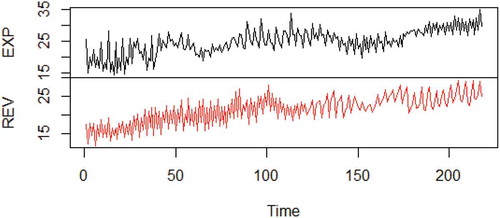
Figure 2. Variables in their first difference
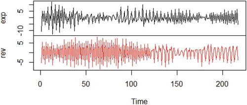
Table 1. Stationary test results
The cointegration results is contained in Table . Before the cointegration test was carried out, lag selection was carried out in order to select the optimal lag length. The test suggests optimal lag order of 8 based on Akaike Information criterion. Since the parameter values of both Trace statistic and Eigen Value Statistic is greater values, we conclude that there exist long-term relationships between the two variables in South African Economy. This suggests the presence of at least one causal relationship between the two variables. Hence, we carried out linear Granger Causality Test.
Table 2. Cointegration test results
The results of linear Granger causality are included in Table . The results show that there exists no causality between government expenditure and government revenue. The absence of linear Granger causality is further affirmed by the results of the variance decomposition and impulse response analysis of the SVAR model. Figure shows show that shocks to government expenditure account for 100% variation in government expenditure and shocks to government revenue does account for 100% variation in government revenue. In other words, the only source of variation in each of the variable is their respective shocks. However, the absence of linear Granger causality is at variance with cointegration theory that states that if two or more variables are cointegrated, there is linear Granger causality in at least one direction. This might be as a result of the nonlinear structure of government expenditure and government revenue. Consequently, we investigate the nonlinear relationship between the two variables.
Figure 3. SVAR variance decomposition.
Table 3. Linear granger causality test results
4.2. Nonlinearity test
We first carried out preliminary nonlinear test by investigating likelihood of nonlinearities using the locally linear autoregressive fit plot of each of the variable as shown by Figures & and the respective RMSE as also shown by Figures & . The results clearly suggest the possibility of the nonlinearities of the two variables. Both BDS test and Mcleod-Li test also confirmed the nonlinearities in the variables. The respective p-value was found to be significant and so the null hypothesis of linearity was rejected. The results of the BDS test and Mcleod–Li test are contained in Tables and respectively.
Figure 4. Local linear autoregressive plot of expenditure.

Figure 5. RMSE of local linear fit of expenditure.
Figure 6. Local linear autoregressive plot of revenue.
Figure 7. RMSE of local linear fit of revenue.
Table 4. BDS nonlinearity test
Table 5. Mcleod–Li test nonlinearity test
4.3. Nonlinear Granger causality results
Having established the nonlinearity in the structure of our variables, we carried out the nonlinear Granger causality test and is contained in Table . The results show that there exists a unidirectional causality running from revenue to expenditure while expenditure is found not to be causal factor of government revenue. In other words, our findings support the tax-spend hypothesis which argues that causality runs from government revenue to government expenditure.
Table 6. Noninear Granger causality test results
4.4. TVAR results
Having confirmed the unidirectional causality from government revenue to government expenditure, the next task is to examine the asymmetric effects of the two variables. As a result, we make use of TVAR model to capture the relationships between the two variables. The TVAR model is a nonlinear multivariate system and has the additive ability to simulate nonlinearity. The model is estimated using R under the package tsDyn. Before the estimation of TVAR, we first carried out LR test available under the same package to test the nonlinearity in VAR with the null hypothesis of linearity in VAR. The results of LR test is presented in Table . The results showed that the null hypothesis of linear VAR is rejected. This means there is at least one threshold in the data. The results also show that TVAR with one threshold is accepted. Hence, we estimate a TVAR with one threshold and revenue serves as threshold variable based on the nonlinear causal relation.
Table 7. LR test
The threshold variables and the threshold values of the constructed TVAR model is presented in Figure . The very top panel depicts the threshold variables of the government revenue. The detected ordered threshold variables and the threshold value which is determined by the Sum of Squared Residuals (SSR) are presented in Figure . The threshold value is 4.9 at the lowest value of the Sum of the Squared Residual.
Given this threshold value, expenditure–revenue relation varies with the identified regime which is divided into two. When revenue as a percentage of GDP is less or equal to 4.9 marks the first regime and include 85.2% of the observed values. Hence, this regime can be said to be “lower revenue regime”. The second regime takes place when revenue is more than 4.9 and includes 18.4% of the observed values and is denoted as the higher revenue regime. From Table , the results show that the main influence of government expenditure and revenue in the lower revenue regime emanate from the autoregressive part. None of the variables has the significant impact on each other in lower revenue regime. Whereas in the higher revenue regime, government expenditure is significantly influenced by revenue while the main influence of revenue is from its own autoregressive.
Figure 8. Threshold value results of the grid search procedure.
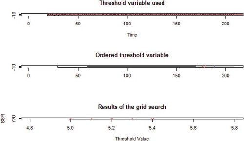
Table 8. TVAR results test
4.5. TVECM results
Based on the linear cointegration result, one could argue that there exists a stable equilibrium in the long-run relationship between government expenditure and revenue. Nevertheless, the changes in government expenditure and government revenues are nonlinear based on the nonlinearity test and nonlinear causality test which was also confirmed by the TVAR model. Consequently, adjustment in any of the variable to the equilibrium suggests the possibility of being asymmetric.
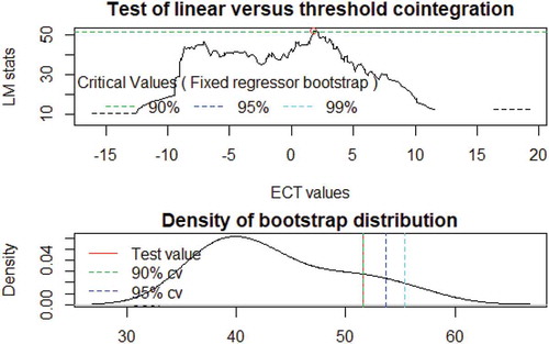
As a result, we make use of the Hansen and Seo (Citation2002) threshold cointegration test with the null hypothesis of linear cointegration in order to determine the presence of asymmetric or threshold in the cointegration relationship between the variables. The result is presented in Table while Figure shows the Hansen and Seo cointegration plot. The results show that the null hypothesis of linear cointegration is rejected because of the significance of the p-value. This means that the long-run relationship between government expenditure and government revenue in South Africa is nonlinear. The estimated cointegration relationship shows that a rise in government revenue by 10% would increase the government expenditure by 18.5% and the estimated threshold cointegration value is 1.7851. According to this value, the model can be divided into two regimes. The TVECM results are presented in Table . The first regime occurs below the threshold cointegration value of 1.7851 and this regime includes 31.2% of the observed values and is normally defined as the extreme regime. While the second regime occurs above the threshold cointegration value and this includes 68.8% observed values and is known as typical regime. From Table , only the error-correction effect in the expenditure equation in the typical region is statistically significant at 1%. However, in the extreme region, none of the error-correction effect is significant statistically in both expenditure and revenue equations. This means that expenditure and revenue deviation from equilibrium will only be accompanied adjustment coefficients in the typical region with the estimated coefficient of 2.9251. Also, the results show that deviation of revenue from the equilibrium state is not followed by the adjustment process to the long-term equilibrium though is not statistically significant. This is particularly important for the government. In a bid to maintain or increase their revenue level, sound fiscal policy measures must be made to prevent reduction of government revenue from the long-term equilibrium state. Empirical findings also suggest that the co-movement of government expenditure and revenue is nonlinear.
Figure 9. Hansen and Seo co-integration plot.
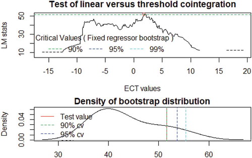
Table 9. Hansen and Seo threshold co-integration
Table 10. TVECM results test
4.6. Markov Regime switching model results
Univariate analysis of each of the variables was done within the framework of Markov Switching model. Our analysis was limited to two regimes because it better fits macroeconomic relationships. Markov Switching model is employed here mainly to determine the persistence of each of the variable in each regime and their corresponding smoothened transition probabilities. The result shows that the probability that government expenditure remains in the regime 1 is 0.5996 while the probability that it remains in regime two is 0.9090. By implication, government expenditure is more persistent in regime 2 than regime 1. Put differently, the probability that government expenditure switches from regime one to regime two is 0.4004 while the probability that it switches from regime 2 to regime 1 is 0.091. This means that government expenditure had tendency to remain in regime 2 which is the regime of high government expenditure. This finding is further confirmed by steady-state probabilities which is the unconditional probability that the system remains in its current regime. The results show that there is 18.5% probability that government expenditure will remain in low regime while 81.5% tendency that it will remain in high regime.
On the other hand, the probability that government revenue remains in the regime 1 is 0.3362 while the probability that it remains in regime two is 0.2283. This shows that government revenue is more persistent in regime one. In other words, government revenue has higher probability of switching from regime 2 to regime 1. This shows that government revenue has tendency of remaining in regime 1 which is regime of low government revenue. Also, the steady-state probabilities show that there is 53.7% probability that government revenue will remain in low regime while 46.3% tendency that it will remain in high regime. This finding is particularly of significance to the fiscal authority to put in place measures to improve and diversify the revenue of the government while putting in place measures to cut wasteful and unnecessary expenses. These empirical findings are illustrated in smoothened transition probability plots of Figures & for both government expenditure and revenue respectively and Table .
Figure 10. Smoothened probabilities for government expenditure.
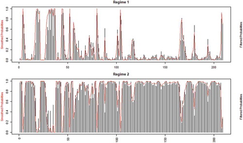
Figure 11. Smoothened probabilities for government expenditure.
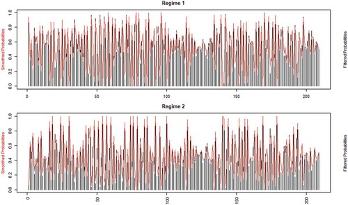
Table 11. Markov switching probabilities
5. Concluding remarks
The study examines the nexus between the government expenditure and revenue in South African economy, using government expenditure as a percentage of GDP and revenue as a percentage of GDP within the nonlinear framework. Quarterly data from 1965(01) to 2019(02) were sourced from the South African Reserve Bank. The results of the linear granger causality showed that there exists no causality between the two variables despite the existence of cointegration. This motivated the need to examine the nonlinearity structure of the variables. Interestingly, several tests of linearity employed in the study suggest the existence of nonlinearity in the structure of the variables. Nonlinear granger causality test was carried out and the empirical findings show that causality runs from government revenue to government expenditure and not vice versa. This provides evidence in support of tax-spend hypothesis. The study then investigated the nonlinearity in VAR with the null hypothesis of linearity in VAR using LR test. The hypothesis of linearity in VAR was rejected as the LR statistics was found to be significant. Hence, the study estimated Threshold Vector Autoregressive (TVAR) with one threshold, and revenue serves as threshold variable given the nonlinear causal relation. The results showed the threshold value is 4.9 when the Sum of the Squared Residual is at its minimum. Empirical findings suggest that in the higher revenue regime, government expenditure is significantly influenced by revenue. The likely explanation for this is that during the revenue boom or when the government revenue target is surpassed, corruption and many other wasteful expenditures are encouraged due to weak institutions and this more than often leads to over-bloated government expenditure. The results of the TVECM show that in the extreme region, none of the error-correction effect is statistically significant in both expenditure and revenue equations. On the other hand, only the error-correction effect in the expenditure equation in the typical region is statistically significant. This means that in the typical regime, error-correction term is effective for the adjustments towards the long-run equilibrium only in the expenditure equation. The implication is that in extreme region, when there is deviation of the government expenditure and revenue from the equilibrium, error-correction term is unable to produce adjustment to equilibrium condition. Whereas in the typical region, error correction will adjust to make them reach the long-run equilibrium only in expenditure equation. This suggests the presence of one-way causality from government revenue to government expenditure in the typical region. This further affirms the unidirectional nonlinear causality running from revenue to expenditure. This means that increased government revenue would push up the government expenditure. The Markov Switching model showed that government expenditure has greater tendency to remain in the high regime while government revenue has higher probability of staying at low regime as suggested by transition probabilities. The steady-state probabilities showed that government expenditure has about 81.5% tendency to remain in high regime while government revenue has higher percentage of remaining in low regime with a lower percentage of remaining in high regime.
The finding provides important information on how government should manage the period of high revenue. The revenue during this period of boom should not be mismanaged because it has the tendency to induce government expenditure, and because there is lower tendency that the revenue will remain in that state. The surge in the revenue should be adequately channeled to productive use and development projects. Government should reinforce observing and appraisal units in all relevant policy institutions to monitor and assess the execution and implementation as well as to track deliverables decided on at policy coordination meetings. Government should toughen their medium-term forecast and estimate framework and budget alignment to sectoral policies in a bid to cut waste and managed the growing expenditure. An all-inclusive tax reform such as growing the tax base, scheming and sustaining an inflation-proof tax system, refining tax administration and collection, spending rationalization, and privatization of inefficient state enterprises are vital in creating fiscal policy reliability.
The major limitation of the study is the scope of the study; as is country specific in nature. Future research in the African continent should consider the possibility of panel studies, especially for Southern African countries.
Cover Image
Source: Author.
Additional information
Funding
Notes on contributors
Kazeem Abimbola Sanusi
Sanusi Kazeem Abimbola is at present a research fellow at University of Johannesburg, South Africa. His research interests include nonlinear models, financial economics, and fiscal and monetary policies.
References
- Afonso, A., & Rault, C. (2009). Spend-and-tax: A panel data investigation for the EU. CESifo Working Paper, No. 2705, 1-13. https://www.econstor.eu/bitstream/10419/30639/1/605747156.pdf
- Alm, J., & Embaye, A. (2013). Using panel methods to estimate shadow economies around the world, 1984–1986. Public Finance Review, 41(5), 510-543..
- Almasri, A., & Shukur, G. (2003). An illustration of the causality relation between government spending and revenue using wavelet analysis on Finnish data. Journal of Applied Statistics, 30(5), 571–21. https://doi.org/10.1080/0266476032000053682
- Athanasenas, A., Katrakilidis, C., & Trachanas, E. (2014). Government spending and revenues in the Greek economy: Evidence from nonlinear cointegration. Empirica, 41(2), 365–376. https://doi.org/10.1007/s10663-013-9221-3
- Ayodele, A., & Falokun, G. (2003). The Nigerian economy: Structure and pattern. Lagos University Printoteque Press.
- Baghestani, H., & McNown, R. (1994). Do revenues or expenditures respond to budgetary disequilibria? Southern Economic Journal, 61(2), 311–322. https://doi.org/10.2307/1059979
- Barro, R. J. (1979). On the determination of the public debt. Journal of Political Economy, 87(5, Part 1), 940–971. https://doi.org/10.1086/260807
- Brady, G. L., & Magazzino, C. (2019). Government expenditures and revenues in Italy in a long-run perspective. Journal of Quantitative Economics, 17(2), 361–375. https://doi.org/10.1007/s40953-019-00157-z
- Chang, T., & Ho, Y. H. (2002). A note on testing” tax-and-spend, spend-and-tax or fiscal synchronization”: The case of China. Journal of Economic Development, 27(1), 151–160 https://ideas.repec.org/a/jed/journl/v27y2002i1p151-160.html.
- Dalena, M., & Magazzino, C. (2012). Public expenditure and revenue in Italy, 1862–1993. Economic Notes, 41(3), 145–172. https://doi.org/10.1111/j.1468-0300.2012.00243.x
- Department of Finance, Republic of South Africa. (1996). Growth, employment and redistribution. A Macroeconomic Strategy. www.numsa.org.za.
- Ebrahim, A., Gcabo, R., Khumalo, L., & Pirttilä, J. (2019). Tax research in South Africa (No. 2019/9). WIDER Working Paper.
- Friedman, M. (1978). The limitations of tax limitation. Quadrant, 22(8), 22 https://search.informit.com.au/documentSummary;dn=148513023132864;res=IELIAC.
- Hamilton, J. D. (1989). A new approach to the economic analysis of nonstationary time series and the business cycle. Econometrica: Journal of the Econometric Society, 57(2), 357–384. https://doi.org/10.2307/1912559
- Hansen, B. E., & Seo, B. (2002). Testing for two-regime threshold cointegration in vector error-correction models. Journal of Econometrics, 110(2), 293–318. https://doi.org/10.1016/S0304-4076(02)00097-0
- Ho, Y., & Huang, C. (2009). Tax-spend, spend-tax, or fiscal synchronization: A panel analysis of the Chinese provincial real data. Journal of Economics and Management, 5(2), 257–272 http://www.academia.edu/download/34332899/06.pdf.
- Hong, T. J. (2009). Tax-and-spend or spend-and-tax? Empirical evidence from Malaysia. Asian Academy of Management Journal of Accounting and Finance, 5(1), 107–115 http://web.usm.my/journal/aamjaf/Vol%205-1-2009/5-1-5.pdf.
- Industrial Development Corporation. (2013). South Africa. http://www.idc.co.za
- Industrial Development Corporation. (2019). South Africa. http://www.idc.co.za
- Karlsson, H. K. (2019). Investigation of the time-dependent dynamics between government revenue and expenditure in China: A wavelet approach. Journal of the Asia Pacific Economy, 25(2), 1–20 https://doi.org/10.1080/13547860.2019.1646573.
- Li, X. (2001). Government revenue, government expenditure, and temporal causality: Evidence from China. Applied Economics, 33(4), 485–497. https://doi.org/10.1080/00036840122982
- Magazzino, C. (2014). The relationship between revenue and expenditure in the ASEAN countries. East Asia, 31(3), 203–221. https://doi.org/10.1007/s12140-014-9211-5
- Mahlakoana, T. (2018). Why skill miss match and joblessness stem from failed educational system Business live. www.businesslive.co.za/fm/features/2018-01-25-the-root-of-theschool-placement-problem
- Narayan, P. K. (2005). The government revenue and government expenditure nexus: Empirical evidence from nine Asian countries. Journal of Asian Economics, 15(6), 1203–1216. https://doi.org/10.1016/j.asieco.2004.11.007
- Nyamongo, M. E., Sichei, M. M., & Schoeman, N. J. (2007). Government revenue and expenditure nexus in South Africa. South African Journal of Economic and Management Sciences, 10(2), 256–269. https://doi.org/10.4102/sajems.v10i2.586
- Owoye, O. (1995). The causal relationship between taxes and expenditures in the G7 countries: Cointegration and error-correction models. Applied Economics Letters, 2(1), 19–22. https://doi.org/10.1080/135048595357744
- Park, W. K. (1998). Granger causality between government revenues and expenditures in Korea. Journal of Economic Development, 23(1), 145–155 http://www.jed.or.kr/full-text/23-1/park.PDF.
- Peacock, A. T., & Wiseman, J. (1979). Approaches to the analysis of government expenditure growth. Public Finance Quarterly, 7(1), 3–23. https://doi.org/10.1177/109114217900700101
- Republic of South Africa, Quarterly Bulletin (QB). (2017) South African Reserve Bank.
- Sanusi, K. A., & Akinlo, A. E. (2016). Investigating fiscal dominance in Nigeria. Journal of Sustainable Development, 9(1), 125–131. https://doi.org/10.5539/jsd.v9n1p125
- Toda, H., & Yamamoto, T. (1995). Statistical Inference in Vector Autoregressions with Possibly Integrated Processes. Journal of Econometrics, 66(1–2), 225–250. https://doi.org/10.1016/0304-4076(94)01616-8
- Tong, H. (1983). Threshold models in nonlinear time series analysis. Lecture Notes in Statistics, 21. https://www.springer.com/gp/book/9780387909189
- Wildavsky, A. B., & Caiden, N. (1988). The new politics of the budgetary process. Scott, Foresman.
- Wolde‐Rufael, Y. (2008). The revenue–expenditure nexus: The experience of 13 African countries. African Development Review, 20(2), 273–283. https://doi.org/10.1111/j.1467-8268.2008.00185.x