Monetary de-measurement of taxation using cogni-economic pressure coefficient on a continuous progressivity model: Towards equitable taxation for Kenya

Abstract

Tax derives from subjects’ earnings measured in monetary terms, a principle anchored in financial accounting. The canon of equity, especially the vertical form, sometimes referred to as “ability to pay” remains monetary. However, negating conventional horizontal equity, equal taxable incomes often require employment of different economic rationality levels to earn them depending on the profession or sector the tax payer comes from; hence different cognitive energies are required to generate the same taxable income—disapproving the mere “ability to pay” paradigm. From the Gamma Rationality Measure for the credit unions sector that comprises 67% of Kenyan economic livelihoods and using a combination of econometric and Riemann double integral methods, the income consumption rationality function is derived, from which a Cogni-economic Pressure Coefficient is generated for each income level. The coefficient is used to work out a more equitable tax structure from a continuous progressivity tax model, for greater equity, incidentally securing a boost to productivity and economy canons of tax administration—a global lesson, specific for Kenya.

Keywords:

• gamma rationality measure
• cogni-economic pressure coefficient
• psych-social economic equation
• income consumption rationality function

PUBLIC INTEREST STATEMENT

Different employments, formal or self, require different physical and mental effort even if the earnings are equal. For instance, a medical doctor may spend more mental energy in dispensing his services than an accountant on account of harrowing experiences, psychological risks by virtue of the profession even if input hours are equal to those of the accountant. If they earn the same, it means they employ different income rationality. To be fair (equitable), the Accountant should be taxed more for use of less mental/physical effort. Taxing them equally as horizontal equity suggests means the doctor is suffer more. More tax is payable with increase in income progressively. The rate of tax levy increase with increase in income should be such that the mental and physical effort (cogni-economic pressure) to bring about equity vertically. In fact, employers would be fair to employees by structuring remuneration on this basis.

1. Introduction

Tax levies are hived off monetary incomes of subjects by governments. The norm is for subjects to declare taxable income, hence liability by submitting regular returns to the government tax department for verification and subsequent payment of the tax for purposes of dispensing income redistribution justice (Bönke et al., 2012). An accompanying condition is for the accounts submitted by the tax payer be audited. This means that since a financial audit is monetary in form and substance the tax therefrom is also monetary measured. Increasing income may be taxed progressively or proportionally or regressively. Progressive structures speak to equity while regressive structures are associated with efficiency objective; so equitable tax levies observe horizontal and vertical types of equity (Lindsay, 2016), though this consideration often contradict efficiency (Brendon, 2013). Progressive structures are however considered superior since they also lead to efficiency in case of market failures (Angelopoulos & Asimakopoulos, 2014). Here, the focus is to show that greater taxation equity may be achieved by introducing the cognitive effort dimension in taxation—called monetary de-measurement.

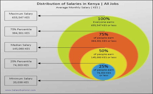
One question begs; and strongly. Is KES 1 earned by a public transport investor in the crazily intricate Kenyan transport industry equal to KES 1 earned by a government employee who reports at 8.00hrs in the morning and retires for the day at 17.00 hours in the evening till the following day? Equivalently, is KES 1 earned by a rice farmer in the Bilharzia infested Mwea Irrigation Scheme equal to KES 1 earned by a wheat farmer in Narok where he needs to visit the farm only four times to harvest their crop? Or, can KES 1 earned by a university professor for teaching 9 hours in a week be compared to KES 1 earned by a doctor on call 24 hours as claimed by horizontal equity (Balestrino et al., 2017)? While consensus is that endowment should be rewarded commensurately, the government is the primary agent for equity and equality through social protection, a notion at the epicenter of the justification for tax levy.

From the above comparatives, it is clear that taxation, which is monetary measured as a derivative of financial statements drawn up using financial accounting principles and as advocated by horizontal equity principle, is a grossly inequitable method of taxation. Some jobs/sectors in the economy require more cognitive effort to earn KES 1 than others. Therefore subjecting all tax payers to the same tax graduated scale rates undermines the very equity which any tax system seeks to achieve. However, it does not mean that the concepts of horizontal and vertical equity concepts in the monetary sense are totally discounted; they do apply where project funding where the attribute concerned is heterogeneous within the scope of study (Barrenho et al., 2017). This paper endeavours to examine how Cogni-economic Pressure Coefficient (CPC)—an extension of the Gamma Rationality Measure, may be used to as a tool provide the much elusive equity needed to evenly distribute the cognitive energy dissipated by an economic agent among tax payers, in order to attain tax equity, and therefore a harmonious society. Progressive taxation has on the most part been used by most countries. Several studies have generated findings that do not conclude on the stability associated with increase in the degree of progression (Fanti & Manfredi, 2003). Unfortunately, the stability addressed has only to do with the tax yield and not the cognitive pressure experienced by economic agents as they go about raising income from which tax is levied.

In the words of Adam Smith in his book The Wealth of Nations (Smith & Stewart, 1963), “The subject of every state ought to contribute towards the support of the government as nearly as possible in proportion to their respective abilities, that is, in proportion to the revenue which they respectively enjoy under the protection of the state”. Of contention is “ … in proportion to the revenue which they respectively enjoy … ” From this statement, arises proportional and progressive tax systems generally in practice by contemporary governments. However, whether proportional or progressive, the monetary measurement aspect remains common in the sense that the cognitive effort employed by subjects in the process of earning the income is not recognized, leading to different perceptions of progressive taxation (Tjondro et al., 2019). Most tax reforms conducted to redistribute tax burden results in the some sectors bearing more burden as others bear less burden after reforms (Salaudeen & Atoyebi, 2018). Yet, the consideration in redistribution has a basis other than the cognitive pressure in financial decision making of economic agents. When this pressure is not evenly or equitably distributed, tax evasion practices become rampant. Corruption means unfairly benefitting from resources not entitled to. Cognitive energy employed to execute corruption for wealth acquisition is much less than that employed fair hard work. Subjects end up getting dissatisfied with the government hence evade payment of tax (Ameyaw & Dzaka, 2016; Drogalas et al., 2018).

Recent tax reform studies suggest that progressive tax structure is preferable with high marginal tax rates at the top and wide tax bands (Diamond & Saez, 2011; Ho & Zhang, 2016) as a more equitable and efficient structure. What is lacking in this empirical claim is how wide the bands should be, whether or not a proportional tax component could be at the tail end of the progression, at what point if so, should the component be introduced, and what, if so, should the proportional tax be. Progressivity is argued to be function of the individual government’s objectives, which will be reflected in taxation policy (Saez, et al., 2012) aligned to the evolutionary market economy goals (Schmiel, 2016). For example, in 1960s, the highest marginal income tax rate ranged about 91% in the United States. This progressivity has been declining since (Piketty & Saez, 2007). Given operational graduated scale rates for Kenya, the aim is to craft a continuous progressivity tax model for Kenya which includes the band width, exemption amounts, and taxation rates parameters. This function is then customized to include individual or sectoral economic rationality dimension. Additionally, an effort has been made to establish the income threshold beyond which a tax payer does not dissipate cognitive energy required to earn for a living. This has been referred to as Reflexive Expenditure Rationality Threshold (RERT). Past this earnings mark, the government may impose an arbitrary proportional tax depending on the economic needs. To this end, a review of the Gamma Rationality Measure (GRM) and the Psycho-social Economic Equation, using the cooperative sector as the hypothetical economy is needful.

By the end of this analysis not only does the canon of equity for both the horizontal and vertical dimensions get revised to avail more evenly distributed economic pressure exertion on taxpayers towards payment of taxes, but also affects the canon of productivity by increasing revenues to the government. Moreover, monetary de-measurement of tax liability by use of cogni-economic pressure coefficient makes a happier taxpayer, which is likely to reduce tax evasion leading to increased efficiency of collection. This speaks to the canon of economy. Implementation of the foregoing recommendations arising from findings enhances equity, productivity and economy in tax administration.

This paper proceeds to first, review the Gamma Rationality Measure (GRM) as the foundation of primary concepts examined hereafter. The relationship between asset turnover and rationality is defined by psychosocial economic equation, the reason why both the measure and the equation are reviewed in series; including relatedness tests and a robustness test. A statement of the problem and objectives will then follow. In methodology, after deriving a continuous tax progressivity model to replace the step function in use including relevant statistical tests, a combination of econometric and Riemann double integration is used to develop the income consumption rationality function from which corresponding cogno-economic pressure coefficients for various incomes derive, and which are used to adjust expected tax yields for various sectors, effectively altering the conventional horizontal equity. Similarly, the income consumption rationality function is used to incorporate cogni-economic pressure coefficients into a revised three level continuous tax yield function that adjust for vertical equity in tax levying.

1.1. Review of the gamma rationality measure and the psycho-social economic equation

Listen honey, if you want to see how people spend their money on things they don’t need, and don’t know how much about what they are getting, and buy it even so without thinking ahead, you would better go study the rich folks. If I wasted money like that, I would be dead. (An ADC mother of eight—personal communication: Excerpt from JM Newton (1977); Economic Rationality of the Poor).

Scholars the world over are in agreement that economic agents are not rational all the time (Simon, 1996). However, little has been done to establish the measure of rationality employed by decision makers of economic and financial decisions. GRM is a measure of rationality level engaged by an economic agent in their ordinary business of survival and wealth creation. Since different personal and corporate endowment levels exist in any economy, some workers scratch their heads more than others to earn a living. This model, developed in 2016, uses Bayesian learning updating process to derive a rationality measure within the continuum of 0% to 100%. By acknowledging that human beings do not regularly update learning, the bivariate Bayesian framework incorporates an additional parameter, updating consistency level (C) (Kirika, 2017). The updating rate is obtained through a Monte Carlo simulation process to derive wealth increases and decreases as additional parameters to generate a three-variable and four-parameter equation to determine rationality. Subjective probabilities are converted into objective probabilities using Cumulative Prospect Theory decision weights function (1992). The Gamma Rationality Equation is thus stated as

(1) $\mathrm{\Gamma }=\frac{cr{p}^i{(1-p)}^d}{r{p}^i{(1-p)}^d+(1-r)q^i{(1-q)}^d}$(1)

where: Г = Gamma Rationality Measure

c = Updating Consistency Level (parameter)

r = Prior rationality level (parameter)

p = Probability of wealth increase after making a rational decision (variable)

q = Probability of wealth increase after making an irrational decision (variable)

i = Number of wealth decreases in a given time interval (parameter)

d = Number of wealth decreases in a given time interval (parameter)

From data, the model showed that low-end income earners struggle more (cognitively) to make KES 1 as compared to high-end income earners. In effect, low-end income earners rationalize their financial/economic decisions higher (i.e. exercise higher rationality) than high-end income earners; confirming the sentiments of the mother of eight in Newton’s (1977) findings in the Rationality of the Poor. Moreover, more educated persons possess a higher potential (entropy) of making more rational decisions but by reason of easier means of earning a living on account of higher salaries, they do not exercise it.

1.2. The psycho-social economic equation (PEE)

This equation derives from the argument that higher rationality exercise in financial decision making invariably brings about higher asset or wealth turnover. This means that if A exercises a rationality of 70% compared to B exercising rationality at 50%, given the same initial capital of KES 1, and the same interval of time, A will have generated more assets than B by expiry of the time interval (Kirika, 2017). This equation creates the link between rationality and wealth creation. For the hypothetical economy, the PEE was found to be

(2) $\begin{array}{rl}& \mathrm{W}\mathrm{t}=27.494\mathrm{l}\mathrm{n}\mathrm{\Gamma }+21.057\\ & {\mathrm{R}}^2=0.799\end{array}$(2)

The coefficient 27.494 is the learning rate coefficient while the constant 21.057 is the maximum asset turnover at 100% rationality as shown in Table 1. The linear equation derived from data had a raw R² of 0.779. These findings are illustrated in figure 1.

Figure 1. Psycho-social economic equation of deposit-taking SACCOs hypothetical economy.

Source: Determinants of Financial Decision Making Rationality in Deposit-taking Cooperatives in Kenya (Kirika, 2017)

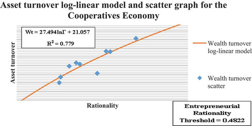
Table 1. Asset turnover from data by the psychosocial economic equation—model

Avg Rat	AT data	AT model
0.5744	7.861	5.8135
0.5654	5.33	5.3793
0.6064	8.628	7.3041
0.7634	14.286	13.6344
0.6959	11.22	11.0891
0.6159	8.334	7.7315
0.6851	11.31	10.6590
0.6618	6.19	9.7077
0.562	4.026	5.2135

Source: Researcher findings (2017)

Levene’s test for robustness and Wilcoxon test for curvilinear correlation between data and the model was conducted as summarized in Tables 2 and 3 respectively. Since the level of significance for the parametric Levene’s test is 0.986, above 0.05, the null hypothesis of equality of variances is retained to mean that the model function is sufficiently robust.

Table 2. Levene’s test of homogeneity of variance between data and turnover model

		Levene Statistic	df1	df2	Sig.
tnover	Based on Mean	.000	1	16	.986
	Based on Median	.007	1	16	.934
	Based on Median and with adjusted df	.007	1	15.696	.934
	Based on trimmed mean	.001	1	16	.982

Source: Researcher findings 2019

Table 3. Wilcoxon, Friedman and Kendall’s tests between data and the asset turnover model

	Null Hypothesis	Test	Sig.	Decision
1	The median of the differences between ATdat and ATmod equals 0.	Related-Samples Sign Test	.508	Retain the null hypothesis
2	The median of the differences between ATdat and ATmod equals 0.	Related-Samples Wilcoxon Signed Rank Test	.859	Retain the null hypothesis
3	The median of the differences between ATdat and ATmod equals 0.	Related-Samples Friedman’s Two-Way Analysis of Variance by Ranks	.317	Retain the null hypothesis
4	The median of the differences between ATdat and ATmod equals 0.	Related-Samples Kendall’s Coefficient of Concordance	.317	Retain the null hypothesis

Asymptotic significance are displayed. The significance level is.05

1Exact significance is displayed for this test.

Source: Researcher findings (2019)

Of key note is that the learning rate coefficient of 27.494 only increases with competition, while the constant term 21.057—the economic fertility constant decreases with competition. This is in line with the fact that more rationality is required in more competitive economies. The term 27.494lnГ is always negative with a maximum of zero at a rationality of 100% which is quite improbable on account of intrinsic irrationality—the source of bounded rationality (Atkinson, 1994; Simon, 1996). At 100% level of rationality, the asset turnover is maximum, posting a turnover of 21.057 over 10 years. The corresponding return on assets is 35.62%. This means that a lending rate beyond this point is infeasible, for nobody can afford such repayment interest rate in the hypothetical economy.

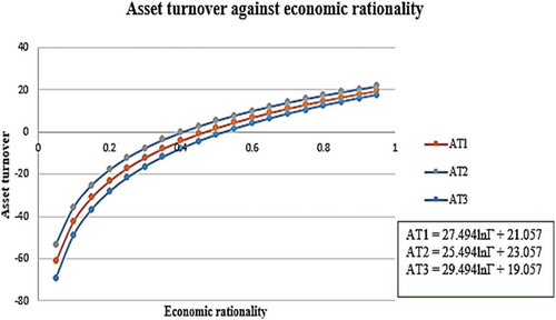
Asset Turnover 1(AT1) an Entrepreneurial Rationality Threshold (ERT) of 48.22%. Meanwhile, AT2 and AT3 post ERTs of 42.1% and 54.21% respectively. This means that one needs to rationalize only 42.1% of all individual financial/economic decisions to survive in Economy 1 etc. AT1, AT2 and AT3 represent Asset turnover in Economy 1, 2 and 3 respectively. Ordinarily, workers migrate from high ERT economies to low ERT economies or sub-economies where they would use their higher rationality to generate a more comfortable life. Equivalently, organizations innovate to engage higher corporate rationalities to survive in current economies or shift to less ERT economies just like workers. Persons operating at lower rationalities than ERT values are dependents in an economy. Those operating at between AT values of between 0 and 1 feed on their own reserves without creating any wealth while those operating at below AT values of below 0 are total dependents on others. Note also that since no one alive can post a rationality of 0 by reason of reflexive rationality (Wilthagen, 1994) the graphs are asymptotic to y-axis. A summary of this notion is shown in figure 2.

Figure 2. Psychosocial economic equations of various economic fertilities.

2. Statement of the problem and objectives

Progressive tax structures are regarded as the cure for inequity and inequality. But they can only address inequity to a limited extent. Other factors that come into play include the population structure but most importantly the income structure. More often, therefore, government policy carries the day. The fiscal objectives of the government dictate the tax policy, so that the amount of work involved to achieve the objectives should most equitably be divided between the various players. Players corporate in terms of public service and private entities finally cascade into individual natural person workers. Given a tax progressivity policy in terms of tax graduated scale rates, the assumption is that the middle income earner is the reference point, with horizontal and vertical equity being fundamental objectives of the policy (McDaniel & Repetti, 1993).

A grave anomaly emerges here. Cognitive energies required to earn KES 1 are different in different sectors of the economy. So, horizontal equity as described in the words “similarly situated” (Elkins, 2006), does not work. The contention is the measure of well-being for purposes of application of horizontal equity. Consequently, the submission here is that well-being should be measured in terms of the cognitive energy exerted during generation of income from which tax should be levied. This has been named income generation rationality, while cognitive energies dissipated during consumption of disposable income is called consumption generation rationality. Additionally, the manner of formulating graduated scale rates vertically, should bring about equality of cognitive pressure of individuals within the economy, which is not necessarily the case. This faults vertical equity. In particular, this paper’s four objectives include: one, to estimate a continuous tax progressivity model which allows for Riemann integrability analysis; that will be equivalent to the operational graduated scale rates for year 2019. Secondly, it seeks to discount horizontal equity by introducing cogni-economic pressure coefficients for discrete economic sectors of a hypothetical economy of deposit-taking cooperatives in Kenya. Thirdly, the income consumption rationality function is formulated. Finally, it derives a continuous progressivity function compliant with cogni-economic pressure coefficients of income, which adjusts for vertical equity.

3. Methodology and discussion

Kenyan graduated tax rates which the hypothetical economy uses, apes an exponential function. And, like many other progressive tax structures, it entails an exemption portion of income followed by three bands equidistant from one another. Tax rates of 15% from KES 161,832 to KES 286,620; 20% from KES 286,621 to KES 425,664 and 25% from KES 425,665 to KES 564,708 apply. But a preceding tax band of 10% is fully covered by the exemption in the name of monthly tax relief which partially encroaches the 15% tax band. Finally, a proportional tax is levied at 30% on all amounts above KES 564,708. This information is summarized in Table 4.

Table 4. Income tax graduated scale rates 2019 individual tax bands and rates

	Annual	Monthly	Rates
On the first	KES 147,580	KES 12,298	10%
On the next	KES 139,043	KES 11,587	15%
On the next	KES 139,043	KES 11,587	20%
On the next	KES 139,043	KES 11,587	25%
On all Income Over	KES 564, 709	KES. 47,059	30%

Monthly Personal Relief KES 1408; Annual Relief KES 16,896

A continuous progressivity model from the exponential functions family may look like:

(1) $y=a{e}^{mx}-s$(1)

Where: y = tax liability and x = taxable income. Letters a, m and s are parameters to be determined. This has been applied on the progressive portion of the tax rate, so that the proportional tax at the high tail end will a separate level of the tax function. A quadratic function model could have been used. Since the exponential function is richer in properties and they yield the same levels of estimation efficiency, the exponential function was preferred.

Using the end points of each tax band, at tax rates of 15%, 20% and 25%, the following three equations obtain. These equations are then solved simultaneously to determine the three parameters:

(2) $18,718.5=a{e}^{286,623m}-s$(2)

(3) $46,527.1=a{e}^{425,666m}-s$(3)

(4) $81,287.85=a{e}^{564,709m}-s$(4)

Adding s to both sides in the three equations yields:

(5) $18,718.5+s=a{e}^{286,623m}$(5)

(6) $46,527.1+s=a{e}^{425,666m}$(6)

(7) $81,287.85+s=a{e}^{564,709m}$(7)

Taking natural logarithms of both sides and subtracting (5) from (6) and (6) from (7) to obtain eliminate log a gives

(8) $ln(46,527.1+s)-ln(18,718.5+s)=139,043m$(8)

(9) $ln(81,287.85+s)-ln(46,527.1+s)=139,043m$(9)

So that (8) and (9) are equated to determine s after eliminating m.

(10) $ln\left\{\frac{46,527.1+s}{18,718.5+s}\right\}=ln\left\{\frac{81,287.85+s}{46,527.1+s}\right\}$(10)

The resulting quadratic equation that reduces to a simple equation obtains s equal to 92,315.9 after simulation. Substituting for s in (5) and (6) and taking natural logs of both sides gives

m = 1.6048528 x 10⁻⁶

This may be substituted back in any of the three original equations to get the value of a as 70,221.3.

(11) $t=70,221.3e^{1.6048528\times {10}^{-6}x}-92,315.9$(11)

The resulting Riemann integrable function (11) can be used to forecast tax liability at 98.5% accuracy level. Assuming that every income level is occupied by a taxpayer, the area under this curve can be worked out thus

$T=\underset{161,833}{\overset{564,709}{\int }}\left(70,221.3e^{1.6048528\times {10}^{-6}x}-92,315.9\right)dx$

${\left.T=\frac{70,221.3}{1.6048528\times {10}^{-6}}{e}^{1.6048528\times {10}^{-6}x}-92,315.9x\right|}_{161,833}^{564,709}$

5.616722278 x 10¹⁰–4.179220479 x 10¹⁰ = 14,375,017,990

where x = gross income and T = Tax yield.

Comparing with the graduated scale rates, the function forms three trapezia whose area can be worked out thus

(12) $\begin{array}{rl}& Y=\frac{1}{2}(286,623-161,833)18,718.5+\frac{1}{2}(425,666-286,623)(46,527.1+18,718.5)\\ & +\frac{1}{2}(564,709-425,666)(81,287.85+46,527.1)=14,589,799,830\end{array}$(12)

Parametric Levene’s test for robustness of the function was also done as shown in Table 6, including Wilcoxon rank test and Kendall’s coefficient of concordance in Table 7, all of which confirmed stability (at a significance level of 0.998 based on mean) and suitability (where the null hypothesis should be retained at 95% level of confidence) of the function. Differential and progressivity model tax liabilities in Table 4 were used. Therefore, the overall Riemann integrable function may be deemed correctly stated in equation (11)(11) $t=70,221.3e^{1.6048528\times {10}^{-6}x}-92,315.9$(11) for purposes of forecasting tax liability.

Table 5. Differential and progressivity model tax liability

Income in KES	240,000	288,000	336,000	384,000	432,000	480,000	520,000	540,000	560,000	564,709
Acttax1 in KES	11,725	18,994	28,594	38,194	48,111	60,112	70,112	75,112	80,112	81,524
Mod3tax in KES	10,899	19,165	28,092	37,734	48,148	59,396	69,454	74,731	80,179	81,488

Table 6. Levene’s test of homogeneity of variance between data and tax liability model

		Levene Statistic	df1	df2	Sig.
Tax	Based on Mean	.000	1	18	.998
	Based on Median	.000	1	18	.998
	Based on Median and with adjusted df	.000	1	17.995	.998
	Based on trimmed mean	.000	1	18	.998

Source: Researcher findings (2019)

Table 7. Wilcoxon, Friedman and Kendall’s Test between data and the tax liability model

	Null Hypothesis	Test	Sig.	Decision
1	The median of the differences between acttax1 and mod3tax equals 0.	Related-Samples Sign Test	.344	Retain the null hypothesis
2	The median of the differences between acttax1 and mod3tax equals 0.	Related-Samples Wilcoxon Signed Rank Test	.059	Retain the null hypothesis
3	The median of the differences between acttax1 and mod3tax equals 0.	Related-Samples Friedman’s Two-Way Analysis of Variance by Ranks	.206	Retain the null hypothesis
4	The median of the differences between acttax1 and mod3tax equals 0.	Related-Samples Kendall’s Coefficient of Concordance	.206	Retain the null hypothesis

Asymptotic significances are displayed. The significance level is .05

¹Exact significance is displayed for this test

Source: Researcher findings (2019)

Predominantly, horizontal equity is interpreted to mean equal tax liability for equal income. However, from the argument adduced, different taxpayers suffer different cognitive pressures during their production processes arising from different attributes of economic sectors they work in, although they may receive equal wages. To address this anomaly, an assumption was made that the tax levy payable was targeting the average taxpayer’s rationality.

On the basis of this assumption, the average rationality sector-wise for the hypothetical economy has been calculated. Sectors employing a higher than average rationality indicate suffering more than the average person in the economy. Consequently, such persons should proportionately pay less tax than a person earning an equal amount, but employing less rationality to generate it. To this end a Cogni-economic Pressure Coefficient (CPC) is calculated thus;

(13) $\mathrm{C}\mathrm{P}\mathrm{C}=\frac{2\mathrm{M}\mathrm{e}\mathrm{a}\mathrm{n}\mathrm{R}\mathrm{a}\mathrm{t}\mathrm{i}\mathrm{o}\mathrm{n}\mathrm{a}\mathrm{l}\mathrm{i}\mathrm{t}\mathrm{y}-\mathrm{S}\mathrm{e}\mathrm{c}\mathrm{t}\mathrm{o}\mathrm{r}\mathrm{a}\mathrm{l}\mathrm{R}\mathrm{a}\mathrm{t}\mathrm{i}\mathrm{o}\mathrm{n}\mathrm{a}\mathrm{l}\mathrm{i}\mathrm{t}\mathrm{y}}{\mathrm{M}\mathrm{e}\mathrm{a}\mathrm{n}\mathrm{R}\mathrm{a}\mathrm{t}\mathrm{i}\mathrm{o}\mathrm{n}\mathrm{a}\mathrm{l}\mathrm{i}\mathrm{t}\mathrm{y}}$(13)

Using this formula results in Table 8. While the normal tax liability (without using CPC) is shown in the current tax column, CPC adjusted tax liability is shown as CPC Tax. Incidentally, more tax is yielded using CPC adjusted liability since some sectors earn more than others using less rationality than the average. After adjustment, such sectors like Mwalimu National SACCO management is liable to pay more. The superordinate goal is to afford taxpayers equality of economic pressure by adjusting through CPC. Mean rationality equals 0.664.

Table 8. Cogni-economic pressure coefficient adjusted tax liability sector-wise

SACCO Group	Wealth (I)KES	Wealth Turnover	Rat	cpc	ROA	2018 Income	Current Tax	CPC Tax
Unitas Members	140,000	14.286	0.7634	0.8503	0.3046	1,037,073,035	311,121,911	264,556,493
Unitas Mgt	827,386,000	11.22	0.6959	0.9520	0.2735	4,117,735,943,596	1,235,320,783,079	1,176,006,439,430
Stima Members	320,000	8.334	0.6159	1.0725	0.2362	962,578,875	288,773,662	309,699,215
Stima Mgt	23,209,000	11.31	0.6851	0.9682	0.2745	117,053,313,916	35,115,994,175	34,001,037,020
M.N. Members	350,000	6.19	0.6618	1.0033	0.2000	623,812,003	187,143,601	187,768,430
Mwalimu N. Mgt	8,073,526,000	4.026	0.562	1.1536	0.1494	6,417,810,175,009	1,925,343,052,503	2,221,145,301,823
Total							3,196,566,868,930	3,431,914,802,411

Source: Researcher findings (2019)

Wealth turnover column is obtained as a cumulative ten year (2005–2015) annual compounded return on equity (column ROA) from the data collected at the beginning of year 2015. This data has been summarized in Appendix A. On the same breath, 2018 income has been prorated using ROA. For instance, Unitas Members income is determined as 140,000 x 14.286 × 1.3046² x 0.3046 = 1,037,073,035. The factor 1.3046² represents cumulative amounts to end of 2017. The amount is then multiplied with the return rate of 0.3046 to get 2018 income. A corporate tax of 30% is further assumed. In Kenya, the cooperative sector is not taxed at corporate tax rate; this assumption has been made just to draw comparatives. Finally, the normal tax is adjusted using CPC to arrive at the last column.

3.1. Estimation of the income consumption rationality function

The principal argument is that naturally, incomes of individuals drive their expenditure rationality. And, that the incomes are earned by exerting a certain amount of rationality. For instance, an individual with a high income rationalizes a smaller proportion of economic decisions than a low income earner. The high income earner may not suffer much if they lose money on account of faulty decisions as the low income earner would. It means that the direction of causality in this variable analysis is from income to rationality. Income becomes the independent variable while rationality is the dependent variable. Moreover, exercise of rationality by economic agents occurs in two distinct phases; the income phase and the consumption phase. In the income phase, the self-employed economic agent rationalizes investment activities and management of the same to derive income. This characterizes most developing economies (Dawson et al., 2009).

For the formally employed individual, the income phase involves the commitment, diligence, competence, employee financed training and their general conduct in the work place to maintain their current income levels or secure promotion to enhance their incomes. Apparently, less effort to maintain employment (Simon, 1951), hence salary income is required compared to maintaining self-employed income deriving from business enterprises, especially necessity entrepreneurs. Business enterprises are a lot more dynamic than formal employment. The owner bears all the risk, and in case of unforeseen circumstances obtaining like sickness accidents among others, the self-employed suffers in entirety. In the meantime, the formal employee, is cushioned by way of insurance cover, and other benefits embedded in their employment contracts when similar situations arise. They benefit by reason of providing rare skills and competences acquired through higher education which the low income earner may not have accessed; especially in developing countries.

On the other hand the consumption phase entails the cognitive effort employed in organizing consumption activities so that the earned income is spent most efficiently. Again, the high income earner faces less pressure to contrive consumption expenditure to avail minimum losses as would the low income earner especially the necessity entrepreneur unless the income of the high income earner reduces due to unforeseen causes (Meng, 2006). But one question begs; which rationality measure should be greater, income or consumption? In responding to this question, two groups of people in the economy emerge; breadwinners and dependents. Breadwinners are the tax payers while dependents have their livelihoods supported by the breadwinners. A high school student, who is a dependent just requires to apply consumption rationality over the pocket money availed by the guardian, so only consumption rationality applies.

The guardian on the other hand has to ensure stability of their job to support both themselves and the high school student. From the foregoing, a reasonable submission is that consumption rationality is always higher than income rationality for the breadwinner. Sometimes the high school student may need to sweet talk the guardian to secure some item he needs and which would not ordinarily be granted by the guardian. This points to exercise of income rationality. However, this is likely to be higher than the corresponding consumption rationality. In this analysis therefore, taxpayers are regarded to exercise greater consumption rationality than income rationality. Conversely, dependents are expected to exercise higher income rationality than consumption rationality since they do not understand the effort required to earn it. It is also possible for a taxpayer to be a dependent. Take an example of a drunkard father in the African setting. Drinking all the money connotes exercise of little consumption rationality perhaps less than income rationality. Usually, such individuals struggle to keep their jobs. However, after receiving the salary it is all drowned into alcohol. A bed ridden patient consuming more than they earn in hospital bills is also a dependent. A responsible father would apply very high consumption rationality to secure savings for investment or to support his dependents. Therefore, for taxpayers;

(14) $\mathrm{I}\mathrm{n}\mathrm{c}\mathrm{o}\mathrm{m}\mathrm{e}\mathrm{r}\mathrm{a}\mathrm{t}\mathrm{i}\mathrm{o}\mathrm{n}\mathrm{a}\mathrm{l}\mathrm{i}\mathrm{t}\mathrm{y}\le \mathrm{C}\mathrm{o}\mathrm{n}\mathrm{s}\mathrm{u}\mathrm{m}\mathrm{p}\mathrm{t}\mathrm{i}\mathrm{o}\mathrm{n}\mathrm{r}\mathrm{a}\mathrm{t}\mathrm{i}\mathrm{o}\mathrm{n}\mathrm{a}\mathrm{l}\mathrm{i}\mathrm{t}\mathrm{y}$(14)

The craft of a mathematical model that puts these notions in perspective follows. From the hypothetical economy, three independent groups are selected representing individuals. It is not clear the whether the average rationalities they exercise are the highest or lowest. This is to be determined by setting the Kenya tax structure 2019 in use, the reference point. To this end it is important to discuss the boundary conditions of the expected function.

3.1.1. Boundary conditions of the income consumption function

Going by reflexive rationality (Wilthagen, 1994), humans possess a minimum amount of rationality inherent and therefore not learned. If a hot metal bar is placed on the wrist of a heathy person, even if unaware, they respond by withdrawing the hand. Not so that they save money to see the doctor over the burn, but to save themselves from pain. In the process of withdrawing the hand, they save the money to see the doctor, which is reflexive. From this, it may be inferred that the income consumption function has no x–intercept. Recall that the y-axis represents Gamma Rationality Measure (GRM). On the dependent variable axis (income/consumption), the function cannot intercept anywhere between 0 and 1, While the maximum is 1, no human being can rationalize at 100%. That is, rationalize all their economic decisions fully (Simon, 1996). It would mean that at zero income, one rationalizes at 100% which is not tenable. This implies that the y-intercept does not exist also. By implication, the function is asymptotic to both axes. These boundary conditions point to a reciprocal function of the form:

(15) $\mathrm{\Gamma }=\frac{a}{Y^b}$(15)

where Γ = Gamma Rationality Measure and Y is disposable income; a and b are parameters to be determined. Using the three independent groups’ annual income data for year 2010 and linearizing equation (15)(15) $\mathrm{\Gamma }=\frac{a}{Y^b}$(15) , the reciprocal term Γ is plotted against 1/Y^b by linear regression. The first SPSS output where b = 1 is presented below.

Table

Model Summary
Model	R	R Square	Adjusted R Square	Std. Error of the Estimate
1	.972^a	.944	.889	.0530087

a) Predictors: (Constant), Y

Table

ANOVA^a
Model			Sum of Squares		df	Mean Square		F		Sig.
1	Regression		.048		1	.048		16.976		.152^b
	Residual		.003		1	.003
	Total		.051		2
Coefficients^a
Model		Unstandardized Coefficients					Standardized Coefficients		t		Sig.
		B		Std. Error			Beta
1	(Constant)	.923		.139					6.642		.095
	Y	7.210E-7		.000			.972		4.120		.152

a. Dependent Variable: 1/Γ

b. Predictors: (Constant), Y

From the above output, neither was the constant significant at either 0.05 or 0.01, nor the coefficient. For this reason, simulation was employed and various values of b tried to increase the level of significance for both the constant and the coefficient. Finally, the best estimate of the function is represented by the output below.

Table

Model Summary
Model	R	R Square	Adjusted R Square	Std. Error of the Estimate
1	.978^a	.956	.911	.0016594

a. Predictors: (Constant), Y

Table

ANOVA^a
Model		Sum of Squares	df	Mean Square	F	Sig.
1	Regression	.000	1	.000	21.508	.135^b
	Residual	.000	1	.000
	Total	.000	2

a. Dependent Variable: 1/Γ^0.05

b. Predictors: (Constant), Y

Table

Coefficients^a
Model		Unstandardized Coefficients		Standardized Coefficients	t	Sig.
		B	Std. Error	Beta
1	(Constant)	1.000	.004		229.871	.003
	Nat	2.541E-8	.000	.978	4.638	.135

a) Dependent Variable: 1/Γ^0.05

The constant turns out significant at below 0.01 but the coefficient is still not significant. Recall that only two values need to define a straight line uniquely, the gradient and the y-intercept. So the intercept is correctly estimated but not the coefficient. Luckily, the functional form has already been determined.

Next is to invoke the Psycho-social Economic Equation. For one to be a tax payer, they must rationalize above 48.22% of all their financial decisions. Furthermore, there exists a minimum rationality level he needs to employ for him to manage to pay the tax. To determine this minimum rationality level, double integration of the resulting function from the above output is done, while retaining the malfunctioning coefficient as the unknown to be determined then equate the overall equation to the tax yield desired in equation (12)(12) $\begin{array}{rl}& Y=\frac{1}{2}(286,623-161,833)18,718.5+\frac{1}{2}(425,666-286,623)(46,527.1+18,718.5)\\ & +\frac{1}{2}(564,709-425,666)(81,287.85+46,527.1)=14,589,799,830\end{array}$(12) . The resulting equation is

(16) $t=y-h({\mathrm{\Gamma }}^{-0.05}-1)$(16)

(17) $T=\underset{161,833}{\overset{564,709}{\int }}\underset{0.4822}{\overset{1}{\int }}\left\{y-h({\mathrm{\Gamma }}^{-0.05}-1)\right\}d\mathrm{\Gamma }dy=14,589,808,212$(17)

$\underset{161,833}{\overset{564,709}{\int }}{\left.\left\{y\mathrm{\Gamma }-h(\frac{{\mathrm{\Gamma }}^{0.95}}{0.95}-\mathrm{\Gamma })\right\}\right|}_{0.4822}^{1}dy=14,589,808,212$

$\underset{161,833}{\overset{564,709}{\int }}\left\{0.5178y-0.0084h\right\}dy=14,589,808,212$

${\left.0.2589y^2-0.0084hy\right|}_{161,833}^{564,708}$

$h=18,081,793.5$

(18) $y-t=18,081,793.5{\mathrm{\Gamma }}^{-0.05}-18,081793.5$(18)

Equation (17)(17) $T=\underset{161,833}{\overset{564,709}{\int }}\underset{0.4822}{\overset{1}{\int }}\left\{y-h({\mathrm{\Gamma }}^{-0.05}-1)\right\}d\mathrm{\Gamma }dy=14,589,808,212$(17) is asking one question. What is the value of h such that taxpayers rationalizing between 48.22% and 100% of their decisions and who earn between KES 161,833 and KES 564,709 are able to pay a total of KES 14.589, 808,212? The assumption here is that at every income level, there is a taxpayer earning the amount. 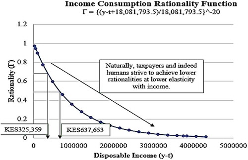Equation (18)(18) $y-t=18,081,793.5{\mathrm{\Gamma }}^{-0.05}-18,081793.5$(18) gives the income consumption rationality function in figure 3, where y-t is the disposable income (net income after tax) and Γ is the Gamma Rationality Measure. A summary of the rationalities used and derived follows in Table 9.

Figure 3. Income consumption rationality function.

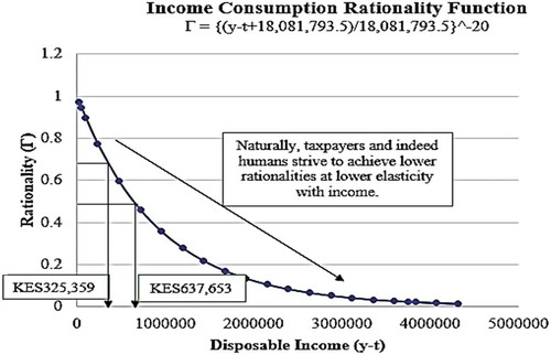
Table 9. Annual disposable income and rationality

Annual Disposable Income (KES)	Average Rationality	Income Rationality	Consumption Rationality
529,155.55	0.7634	0.5616	0.7819
923,797.38	0.6159	0.3691	0.6385
870,789.87	0.6618	0.3904	0.6867

Average rationality = Income rationality x proportion of investment + Consumption rationality x proportion of consumption. Any amounts saved are assumed to have been invested. Evidently, income rationality is less than consumption rationality.

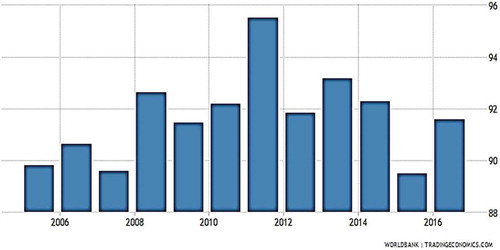
Using 2016 percentage consumption of GDP (91.6%) as personal consumption proportion, consumption column is filled and highlighted as shown in figure 4. A taxpayer rationalizing income at 50% and rationalizing consumption at 70%, is able to save 49% of income. But if the taxpayer exercises equal income to consumption rationality, no saving is made. Worse still, if the taxpayer rationalizes their consumption process lower than the income, they can only be a dependent; since it would mean they spend more than what is earned—living beyond their means. The income consumption rationality function forms the basis of subsequent modelling whereby a continuous progressivity model for the entire income range is developed incorporating the cogni-economic pressure coefficients for every income level. A CPC adjusted tax schedule comparing with the current tax computation is presented; resulting in 14% tax increase.

Figure 4. Kenya’s consumption proportion of GDP 2006–2016 in percentage.

Source: World Bank data Tradingeconomics.com (2019)

Finally, assuming that the tax rates were referenced on the median income earner using figure 5, the median taxpayer is assigned a rationality value of one. Any taxpayer rationalizing incomes at higher than the median tax payer, an appropriate value less than one is assigned. And, any taxpayer rationalizing income at lower than the median taxpayer is assigned a value greater than one. To this end, since the income consumption function—equation (18)(18) $y-t=18,081,793.5{\mathrm{\Gamma }}^{-0.05}-18,081793.5$(18) is a non-linear reciprocal function of order power −20, to make it linear, the opposite, that is, raising it to power −0.05 is required. This operation leads to the following equation:

(19) $CPC={\left\{\frac{\mathrm{M}\mathrm{e}\mathrm{d}\mathrm{i}\mathrm{a}\mathrm{n}\mathrm{i}\mathrm{n}\mathrm{c}\mathrm{o}\mathrm{m}\mathrm{e}\mathrm{r}\mathrm{a}\mathrm{t}\mathrm{i}\mathrm{o}\mathrm{n}\mathrm{a}\mathrm{l}\mathrm{i}\mathrm{t}\mathrm{y}}{Re\mathrm{q}\mathrm{u}\mathrm{i}\mathrm{r}\mathrm{e}\mathrm{d}\mathrm{i}\mathrm{n}\mathrm{c}\mathrm{o}\mathrm{m}\mathrm{e}\mathrm{r}\mathrm{a}\mathrm{t}\mathrm{i}\mathrm{o}\mathrm{n}\mathrm{a}\mathrm{l}\mathrm{i}\mathrm{t}\mathrm{y}}\right\}}^{0.05}=\frac{0.9326}{{\{\mathrm{R}\mathrm{e}\mathrm{q}\mathrm{u}\mathrm{i}\mathrm{r}\mathrm{e}\mathrm{d}\mathrm{i}\mathrm{n}\mathrm{c}\mathrm{o}\mathrm{m}\mathrm{e}\mathrm{r}\mathrm{a}\mathrm{t}\mathrm{i}\mathrm{o}\mathrm{n}\mathrm{a}\mathrm{l}\mathrm{i}\mathrm{t}\mathrm{y}\}}^{0.05}}$(19)

Using CPC—equation (19)(19) $CPC={\left\{\frac{\mathrm{M}\mathrm{e}\mathrm{d}\mathrm{i}\mathrm{a}\mathrm{n}\mathrm{i}\mathrm{n}\mathrm{c}\mathrm{o}\mathrm{m}\mathrm{e}\mathrm{r}\mathrm{a}\mathrm{t}\mathrm{i}\mathrm{o}\mathrm{n}\mathrm{a}\mathrm{l}\mathrm{i}\mathrm{t}\mathrm{y}}{Re\mathrm{q}\mathrm{u}\mathrm{i}\mathrm{r}\mathrm{e}\mathrm{d}\mathrm{i}\mathrm{n}\mathrm{c}\mathrm{o}\mathrm{m}\mathrm{e}\mathrm{r}\mathrm{a}\mathrm{t}\mathrm{i}\mathrm{o}\mathrm{n}\mathrm{a}\mathrm{l}\mathrm{i}\mathrm{t}\mathrm{y}}\right\}}^{0.05}=\frac{0.9326}{{\{\mathrm{R}\mathrm{e}\mathrm{q}\mathrm{u}\mathrm{i}\mathrm{r}\mathrm{e}\mathrm{d}\mathrm{i}\mathrm{n}\mathrm{c}\mathrm{o}\mathrm{m}\mathrm{e}\mathrm{r}\mathrm{a}\mathrm{t}\mathrm{i}\mathrm{o}\mathrm{n}\mathrm{a}\mathrm{l}\mathrm{i}\mathrm{t}\mathrm{y}\}}^{0.05}}$(19) , tax liabilities are adjusted so that the three equations (2)(2) $\begin{array}{rl}& \mathrm{W}\mathrm{t}=27.494\mathrm{l}\mathrm{n}\mathrm{\Gamma }+21.057\\ & {\mathrm{R}}^2=0.799\end{array}$(2) , (3(3) $46,527.1=a{e}^{425,666m}-s$(3) ) and (4(4) $81,287.85=a{e}^{564,709m}-s$(4) ) initially used to derive a continuous progressivity function transform into equations (20)(20) $17,715=a{e}^{286,623m}-s$(20) , (21(21) $44,301=a{e}^{425,666m}-s$(21) ) and (22(22) $77,836=a{e}^{564,709m}-s$(22) ).

(20) $17,715=a{e}^{286,623m}-s$(20)

(21) $44,301=a{e}^{425,666m}-s$(21)

(22) $77,836=a{e}^{564,709m}-s$(22)

Solving equations (20)(20) $17,715=a{e}^{286,623m}-s$(20) , (21(21) $44,301=a{e}^{425,666m}-s$(21) ) and (22(22) $77,836=a{e}^{564,709m}-s$(22) ) simultaneously results in:

Figure 5. Salary income distribution in 2019.

Source: Salaryexplorer.com (2019)

$s=83,999.7;a=63,023.3;m=1.600217\times {10}^{-6}$. So that the CPC tax adjusted equation reads:

(23) $t_{cpc}=63,023.3e^{1.600217\times {10}^{-6}x}-83,999.7$(23)

When a schedule comparing the current tax computation with the CPC adjusted (monetary de-measured) tax computation, such an extract looks like the following Table 10.

Table 10. Current Tax and CPC tax comparatives

Income(Y)	Rat	CPC	CPC Tax	Current Tax
161,833	0.8354	0.9410	(1,383)	0
171,810	0.8277	0.9415	0	1,497
181,832	0.8200	0.9419	1,413	3,000
201,832	0.8049	0.9428	4,305	6,000
221,832	0.7902	0.9436	7,297	9,000
241,832	0.7759	0.9445	10,393	12,000
261,832	0.7620	0.9454	13,594	15,000
281,832	0.7484	0.9462	16,906	18,000
286,623	0.7452	0.9464	17,715	18,719
301,832	0.7351	0.9471	20,330	21,760
321,832	0.7222	0.9479	23,873	25,760
341,832	0.7096	0.9487	27,536	29,760
361,832	0.6974	0.9496	31,324	33,760
381,832	0.6854	0.9504	35,242	37,760
401,832	0.6738	0.9512	39,293	41,760
421,832	0.6625	0.9520	43,482	45,760
425,666	0.6603	0.9522	44,301	46,527
441,832	0.6514	0.9528	47,813	50,569
461,832	0.6407	0.9536	52,291	55,569
481,832	0.6303	0.9544	56,921	60,569
501,832	0.6201	0.9552	61,708	65,569
521,832	0.6102	0.9559	66,656	70,569
541,832	0.6006	0.9567	71,772	75,569
561,832	0.5913	0.9574	77,061	80,569
564,708	0.5900	0.9575	77,836	81,288
564,709	0.5900	0.9575	77,836	81,288
664,708	0.5472	0.9611	106,963	111,288
764,708	0.5077	0.9648	136,308	141,288
864,708	0.4711	0.9684	165,869	171,288

Source: Researcher findings (2020)

Tax exempt income rose from KES 161,833 to KES 170,810. This gets us to the following overall CPC adjusted tax function for all incomes:

(24) $t_{cpc}=\left\{\begin{array}{c}0,\hspace{0.17em}\mathrm{\forall }\hspace{0.17em}y\le 171,810\\ 63,023.3e^{1.600217\times {10}^{-6}y}-83,999.7,\hspace{0.17em}\mathrm{\forall }171,810<y\le 564,709\\ 1.0831116\times {10}^{-8}{y}^2+0.27796y-82,585.83,\hspace{0.17em}\mathrm{\forall }y>564,709\end{array}\right.$(24)

A continuous tax progressivity model has been monetary de-measured in the “accounting sense” by incorporating a component that takes care of the cognitive energy dissipated by individual taxpayers in their ordinary business of income generation. This way more equitable tax is levied; addressing anomalies of both horizontal and vertical equity. In the meantime, both the Mwea rice farmer in bilharzia prone regions and the Public transport investor who exert different cognitive energies in income generation are catered for more equitably. At the same time, if they earn different incomes chargeable as income tax, equation (24)(24) $t_{cpc}=\left\{\begin{array}{c}0,\hspace{0.17em}\mathrm{\forall }\hspace{0.17em}y\le 171,810\\ 63,023.3e^{1.600217\times {10}^{-6}y}-83,999.7,\hspace{0.17em}\mathrm{\forall }171,810<y\le 564,709\\ 1.0831116\times {10}^{-8}{y}^2+0.27796y-82,585.83,\hspace{0.17em}\mathrm{\forall }y>564,709\end{array}\right.$(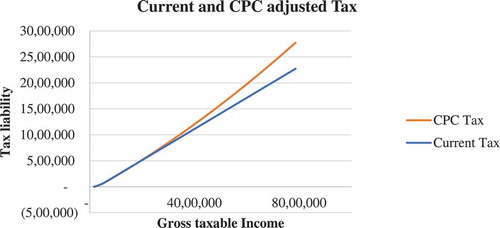24) addresses their cognitive pressures as well. Area under the CPC tax curve for the annual taxable income up to KES 5,176,436 amounts to KES 3,783.5 billion. Comparatively, the current tax area under the curve yields KES 3,565 billion, an increase of 6%.

Incidentally, about 10.7% (appendix B) higher tax yield (levied from higher income earners progressively) results with the CPC tax computation as opposed to the current tax levy system. Note that these are arbitrary choice incomes, while area under the curve is another sweeping assumption that at every income level, there is a tax payer which may not be true. Overall, the assumption is that the taxpayers’ distribution of income position is the same for both the current tax and the CPC adjusted tax. This can be verified by integrating the area under both curves as shown in Figure 6. Income beyond KES 5,176,436 avail through rationalities less than 2.36% which is the reflexive rationality of the group considered (Kirika, 2017). For these amounts the government may levy any proportional tax without the taxpayer feeling any pinch.

Figure 6. Current tax and CPC adjusted tax continuous progressivity functions.

3.2. Limitations of the study

A conspicuous limitation relates to implementation of the policy. The likelihood of politicization of the policy to craft cogni-economic pressure coefficients for each sector is high especially in developing countries like Kenya. With regard to derivation of the income consumption rationality function on which cogni-economic coefficients are anchored, a combination of inexact econometric estimation methods together with unique solution deterministic methods used are likely to render the function slightly inaccurate. Nevertheless, the function may still be regarded a fair approximation of reality; only that continuous research is required to establish the right function parameters as economic agents increase their economic rationalities over time to reflect increasingly challenging cost of living.

3.3. Generalizations

The hypothetical economy is a proper subset of the Kenyan society. About 67% of all Kenyans derive their livelihoods directly or indirectly from SACCO activities (SASRA, 2013). This means that the above models and the assumptions underlying may be generalized for the Kenyan society. With more growth of the cooperative sector, the models discussed gain greater credibility.

4. Conclusion

All the four objectives of this paper stand achieved. First, at 98% accuracy level, the exponential function was able to forecast true tax payable as confirmed by Levene’s test. It is possible to create more accurate models of estimation but this would entail unwarranted rigour. Researchers are invited to explore more precise models with less sophistication. The hypothetical economy was to assist in creating sectors like in a real economy; which it did. For purposes of addressing horizontal equity anomalies the CPC’s for the sectors worked to actually gather more tax for the government enhancing productivity of tax levied after evening cogni-economic pressure, which resonates with the main objective of delivering more horizontal equity.

Perhaps the greatest achievement of this analysis is formulation of the income consumption rationality function. This is hoped to generate a lot more uses in the advancement of the Entropy Rationality Theory and its corollary—Psychosocial Economic Equation. With it was birthed the three types of rationalities, average, income and consumption rationalities. These advances the Gamma Rationality Measure in a huge and unprecedented way. Finally, the income consumption rationality function was used to develop a CPC tax adjusted progressivity function that addresses vertical equity implementation anomalies. Inequity, whichever nature promotes tax evasion which increases administration costs reducing efficiency (King & Sheffrin, 2002). This model therefore is likely to be more economical. Save for administration challenges of the tax models so formulated, they go a long way to expound the perspective in which tax equity should be viewed.

Cover image

Source: Author.

Additional information

Funding

The author received no direct funding for this research.

Notes on contributors

Stanley K. Kirika

The author, a CPA, holds a PhD (Finance) and is the Accounting Team Leader. Quantitative Behavioural Economics/Finance area is his key specialty. This is fairly wide, including application of Bayesian Statistics and Frequentist Statistics/econometric methods in linking classical economics with behavioural economics. No human can survive without rationalizing their financial decisions (Classical Economics); as well, it is impossible to rationalize all economic decisions on account of insufficient information and limited cognitive processing ability (Behavioural Economics). On this premise, the Entropy Rationality Theory/Model (2017) determines the proportion of decisions rationalized by an economic agent – the Gamma Rationality Measure from a combination of geometric Brownian motion (diffusion finance), multi-period Bayesian probability model, cumulative prospect theory (behavioural finance), Accounting Theory, Information Theory and Statistical Entropy. The broad research aim is to use mathematical finance/economics and mathematical statistics to develop models that bridge theoretical Behavioural Economics/Finance with classical economics/finance in personal and corporate financial decision making. This article bridges behavioural human aspects for equitable tax levy.

 

Appendix A.

Table

Current Tax and CPC Adjusted Tax computations
Income(Y) in KES	Rat (Γ)	CPC	Current Tax	CPC Tax
161,833	0.835424	0.941023	0.15	−1382.78
171,810	0.827671	0.941461	1496.55	0.080284
261,832	0.761971	0.945363	14,999.85	13,594.12
281,832	0.74837	0.946214	17,999.85	16,905.53
286,623	0.745164	0.946418	18,718.5	17,715.49
301,832	0.735115	0.94706	21,760.3	20,330.46
421,832	0.662461	0.952001	45,760.3	43,481.84
425,666	0.660325	0.952155	46,527.1	44,300.96
441,832	0.651438	0.9528	50,568.6	47,813.03
461,832	0.640709	0.953592	55,568.6	52,291.21
561,832	0.591292	0.957426	80,568.6	77,060.53
564,708	0.589971	0.957533	81,287.6	77,835.5
564,709	0.589971	0.957533	81,287.85	77,835.77
664,708	0.547195	0.961144	111,287.5	106,963.3
764,708	0.507664	0.964754	141,287.5	136,307.7
864,708	0.471121	0.968364	171,287.5	165,868.7
4,707,330	0.032374	1.107097	1,324,074.1	1,465,879
4,749,976	0.031486	1.108637	1,336,867.9	1,482,101
4,792,622	0.030624	1.110177	1,349,661.7	1,498,363
4,835,268	0.029787	1.111716	1,362,455.5	1,514,664
4,877,914	0.028974	1.113256	1,375,249.3	1,531,005
4,920,560	0.028184	1.114796	1,388,043.1	1,547,384
4,963,206	0.027417	1.116335	1,400,836.9	1,563,804
5,005,852	0.026671	1.117875	1,413,630.7	1,580,263
5,048,498	0.025947	1.119415	1,426,424.5	1,596,761
5,091,144	0.025243	1.120954	1,439,218.3	1,613,298
5,133,790	0.02456	1.122494	1,452,012.1	1,629,875
5,176,436	0.023896	1.124034	1,464,805.9	1,646,491

Source: Researcher findings (2020)

 

 

Appendix B. Operational data summary

	No. of obs. (1)	Avg Age (2)	Educ Level index (3)	Delta (4)	Initial Rat (5)	Current Rat (6)	Indecision rate rd = 2005 (7)	Indecision rate rd 2015 (8)	Pr(Inc|Rat = 0) 2005 (9)	Pr(Inc|Rat = 0) 2015 (10)	Pr(Inc|Rat = 1) 2005 (11)	Pr(Inc|Rat = 1) 2015 (12)	Drift (13)	Std Dev (14)	Wo (Sh’000) Avg (15)
Mwalimu	91	41.0	3.19	0.634	0.7971	0.9808	0.7681	0.7698	0.4540	0.4796	0.8884	0.8483	0.1505	0.2330	350
Female	44	41.4	3.28	0.633	0.8450	0.9836	0.7875	0.8151	0.4817	0.7314	0.8711	0.8562	0.1298	0.2943	350
Male	47	40.6	3.11	0.634	0.7472	0.9781	0.7499	0.7255	0.4294	0.4688	0.9031	0.8296	0.1699	0.1883	350
Mgt	16	38.7		0.633	0.8173	0.8769	0.7329	0.6707	0.8070	0.4681	0.9424	0.8891	0.1540	0.1646	8,073,526
Stima:	47	36.8	2.26	0.634	0.8800	0.9699	0.8505	0.8036	0.4464	0.5778	0.8584	0.8061	0.2814	0.2579	320
Female	15	38.0	2.33	0.636	0.8321	0.9700	0.8993	0.8407	0.4859	0.4859	0.8489	0.7429	0.3703	0.1052	320
Male	32	36.2	2.23	0.633	0.9012	0.9708	0.8215	0.7832	0.4265	0.6205	0.8631	0.8347	0.2577	0.2987	320
Mgt	14	30.5		0.633	0.6866	0.9361	0.5301	0.5111	0.5021	0.6205	0.9319	0.9411	0.3208	0.2304	23,209
Unitas:	133	38.4	1.28	0.632	0.8576	0.9665	0.8274	0.9113	0.5686	0.6237	0.8275	0.8374	0.2889	0.46036	140
Female	66	38.8	1.27	0.632	0.8627	0.9670	0.8162	0.9380	0.7365	0.6831	0.8229	0.8202	0.3341	0.48781	140
Male	67	38.0	1.3	0.633	0.8556	0.9646	0.3956	0.8781	0.4128	0.5740	0.7926	0.8035	0.2536	0.43771	140
Mgt	16	30		0.633	0.5592	0.8934	0.8347	0.7346	0.7171	0.6637	0.8582	0.8835	0.2735	0.09034	827,386
Age:	3	22	2	0.629	0.6246	0.9774	0.0486	0.9999	0.4759	0.8465	0.8465	0.9615
	15	27	2.08	0.644	0.6832	0.9420	0.8690	0.7590	0.3900	0.5493	0.7430	0.7546
	35	32	1.79	0.632	0.9058	0.9811	0.8352	0.8656	0.4031	0.6215	0.8440	0.8724
	47	37	1.74	0.632	0.9012	0.9806	0.8870	0.9234	0.6570	0.7000	0.8385	0.8031
	35	42	1.91	0.632	0.8452	0.9854	0.7336	0.8230	0.3250	0.5152	0.8589	0.8112
	30	47	2.46	0.632	0.8367	0.9476	0.7740	0.7842	0.7360	0.6076	0.6466	0.6767
	17	52	2.24	0.634	0.9483	0.9738	0.8139	0.8519	0.3413	0.2289	0.8786	0.8965
	5	57	2	0.632	0.9768	0.9845	0.8750	0.8750	0.3501	0.3501	0.4428	0.4428
Gender:
Female	125	39.9	1.931	0.633	0.8142	0.9471	0.7817	0.8341	0.5242	0.4811	0.7802	0.7553	0.2735	0.4047	241.7
Male	146	38.9	2.02	0.633	0.8211	0.9438	0.7247	0.7591	0.4229	0.5311	0.7771	0.7544	0.2335	0.3518	241.7
SACCOS Overall	317	39.4	1.98	0.633	0.8182	0.9451	0.7505	0.7739	0.452	0.5104	0.7785	0.7548	0.2508	0.3941	241.7

Notes to table B:

1. Column (4) is a transformation of column (4) of table 4.1 to obtain parameter delta using the equation

2. $\delta =0.69-\{LOT(R)/24\}\ast 0.08$, for the equation: $p_s=\frac{{p_o}^{\delta }}{{\left\{{p_o}^{\delta }+{(1-p_o)}^{\delta }\right\}}^{1/\delta }}$, where p_o and p_s are objective and subjective probabilities respectively (Kahneman and Tversky, 1992).

3. Columns (5) to (12) indicate transformed subjective probabilities into objective probabilities;

4. All other columns remain the same as in table 4.1

5. The sum of 327 represents the total number respondents for the questionnaires. However, they did not respond to all questions; so that some analysis tables will show less than the total indicated in the operational summaries e.g., table 4.3 showing a total of 259. Moreover, analysis of SACCO managements has been done separately, its total respondents being 46. This leaves 281 for SACCO member respondents.

References

- Ameyaw, B., & Dzaka, D. (2016). Determinants of tax evasion: Empirical evidence from Ghana. Modern Economy, 7(14), 1653–26. https://doi.org/10.4236/me.2016.714145
- Angelopoulos, K., & Asimakopoulos, S. (2014). iTax smooth $ ing in a business cycle model with capital and skill complementarity. Journal of Economic Dynamics and Control, (1889). J. Malley, 165.
- Balestrino, A., Grazzini, L., & Luporini, A. (2017). A normative justification of compulsory education. Journal of Population Economics, 30(2), 537–567. https://doi.org/10.1007/s00148-016-0619-7
- Barrenho, E., Miraldo, M., Shaikh, M., & Atun, R. (2017). Vertical and horizontal equity of funding for malaria control: A global multisource funding analysis for 2006–2010. BMJ Global Health, 2(4), e000496. https://doi.org/10.1136/bmjgh-2017-000496
- Bönke, T., Eichfelder, S., & Utz, S. (2012). Uneven treatment of family life? Horizontal equity in the US tax and transfer system (No. 2012/18). Diskussionsbeiträge.
- Brendon, C. (2013). Efficiency, equity, and optimal income taxation.
- Dawson, C. J., Henley, A., & Latreille, P. L. (2009). Why do individuals choose self-employment?
- Drogalas, G., Anagnostopoulou, E., Pazarskis, M., & Petkopoulos, D. (2018). Tax ethics and tax evasion, evidence from Greece. Theoretical Economics Letters, 8(5), 1018–1027. https://doi.org/10.4236/tel.2018.85070
- Elkins, D. (2006). Horizontal equity as a principle of tax theory. Yale Law & Policy Review, 24, 43.
- King, S., & Sheffrin, S. M. (2002). Tax evasion and equity theory: An investigative approach. International Tax and Public Finance, 9(4), 505–521. https://doi.org/10.1023/A:1016528406214
- Kirika, S. K. (2017) Determinants of financial decision making rationality in deposit-taking cooperatives in Kenya [PhD Thesis]. Jomo Kenyatta University of Agriculture and Technology
- Lindsay, I. K. (2016). Tax fairness by convention: A defense of horizontal equity. Florida Tax Review, 19, 79.
- McDaniel, P. R., & Repetti, J. R. (1993). Horizontal and vertical equity: The Musgrave/Kaplow exchange. Florida Tax Review, 1, 607.
- Meng, X. (2006). Unemployment, consumption smoothing and precautionary saving in urban China. In Unemployment, inequality and poverty in urban China (pp. 106–128). Routledge.
- Newton, J. M. (1977). Economic rationality of the poor. Human Organization, 36(1), 50. https://doi.org/10.17730/humo.36.1.2522272541p0kn27
- Piketty, T., & Saez, E. (2007). The impact of economic growth and tax reform on tax revenue and structure: Evidence from China experience.
- Saez, E. (2012). High-tech enterprise tax planning.
- Salaudeen, Y. M., & Atoyebi, T. A. (2018). Tax burden implication of tax reform. Open Journal of Business and Management, 6(3), 761. https://doi.org/10.4236/ojbm.2018.63058
- SASRA. (2013). Deposit taking SACCO societies licensed by the sacco regulatory authority.
- Schmiel, U. (2016). Evolutionary analysis of tax law: A methodological approach. Modern Economy, 7(4), 377–390. https://doi.org/10.4236/me.2016.74041
- Simon, H. A. (1951). A formal theory of the employment relationship. Econometrica: Journal of the Econometric Society, 19(3), 293–305. https://doi.org/10.2307/1906815
- Simon, H. A. (1996). The sciences of the artificial. MIT press.
- Smith, A., & Stewart, D. (1963). An inquiry into the nature and causes of the wealth of nations (Vol. 1). Irwin.
- Tjondro, E., Santosa, K. G., & Prayitno, N. (2019). Perceptions of service-orientation and trust of tax officers between millenials, X, and baby boomers [Doctoral dissertation]. Pascasarjana Mercu Buana Jakarta.
- Zeng, K., Li, S., & Li, Q. (2013). Optimal progressive taxation in a model with endogenous skill supply.