Revisiting the Volatility- Growth relationship: Some cross country evidence, 1978–2017

Abstract

This paper attempts a re-examination of the relationship between the output volatility and economic growth using an annual data set for select 67 countries for the period 1978 to 2017 spanning over 40 years. Towards this objective cross section and panel, regressions are estimated for different country groups namely developing, industrial, high financially integrated (HFI) and low financially integrated (LFI) country groups. Overall, the results indicate that output volatility as a proxy of macroeconomic volatility has negative effect on economic growth. The results appear to be stronger when we include other control variables as part of an information set. The panel regression results support the negative relationship between economic growth and volatility for the developing countries. The financial development indicator indicates significant relation with growth for industrial economies.

Keywords:

• economic growth
• growth volatility
• financial development
• HP filter

Jel Classification:

• C1
• C3
• F15
• F36
• F41
• F43
• G24

PUBLIC INTEREST STATEMENT

In the last few decades, different economies have been relatively more integrated financially preceded by their integration with trade. In this backdrop macroeconomic volatility namely in terms of output volatility has been a major concern for the economies all over the world. Output volatility is found to have an effect on growth in different economies. This paper revisits this debate and finds some contrasting evidence in volatility growth nexus for the developing, high and low financially integrated economies.

1. Introduction

The debate on the volatility and growth relationship gained momentum in the literature in the last two and half decades. We find both theoretical and empirical studies examining this link attributing different sources to volatility. As regards the sources of volatility, Turnovsky Stephen and Chattopadhyay (2003) summarize three key sources of volatility. A negative link between volatility and growth is found by Ramey and Ramey (1995), evidenced in his cross-country exercise. Specifically, the study finds adverse relation between mean output growth rates and their volatility. Later, this work is extended by Fatas (2002), Hnatkovska (2005) among others, wherein the general finding points to volatility in reducing the magnitude of economic growth in general and particularly, in those countries that are financially and institutionally underdeveloped. In terms of business cycle, the relationship is found positive if volatility is associated with occurrence of recession. Recession in turn leads to higher research and development (R&D) or say destruction of least productive firms in Schumpeter’s words (Loayza et al. (2007)¹. This whole process generates higher economic growth alongside higher volatility; see Grier and Tullock (1989), Caporale and McKiernan (1996), and Kormendi and Meguire (1985). Inclusion of other volatility measures yield insignificant impact on output, though positive (Gavin and Hausman, 1995). The second strand of literature investigates the relationship between policy instruments’ volatility and growth. Aizenman and Marion (1993) examine the effect of policy uncertainty on economic growth in the endogenous growth framework with investment irreversibility. First, the investors’ behaviour towards uncertainty about the future affects the long-term growth. Due to uncertainty, firms get wrong signal and tend to invest in a wrong project. Increase in volatility can also lead to reduced investment if the investment is characterised by irreversibility. The authors confirm that policy fluctuations could lead to lower economic growth. Kormendi and Meguire (1985) and Aizenman and Marion (1993) deal with volatility of monetary and fiscal policies affecting output growth. Some of the external sources of volatility such as terms of trade and real exchange rate affecting growth is the engagement in the third strand of literature(Mendoza, 1994, Gavin and Hausman, 1995), but the results are inconclusive on the direction of the relationship.

A few other studies examine the role of financial integration while studying the said growth volatility relationship and related issues. For instance, Mendoza (1994) by applying a stochastic dynamic business cycle model finds that financial integration has little impact on output and consumption volatility. He also notices that volatility rises when the shocks are large and persistent. A few others use dynamic stochastic sticky-price model² to explain the importance of monetary and fiscal shocks on output and consumption volatility. In the presence of monetary and or fiscal policy shocks, the change in output volatility and the change in consumption volatility depend on the degree of financial integration (Sutherland, 1996 and Senay, 1998). Aghion and Saint-pual (1998) find that in recession, the cost involved in innovation decreases, which tends to improve productivity and therefore, yield higher economic growth. Further, Grier and Perry (2000) apply bivariate GRACH-M model to examine the link between uncertainty, inflation, and output growth for United States over the period of 1948 to 1996 and they find no evidence to support the relationship.

Apart from the empirical strands discussed above, the theoretical literature on risk-output-growth relationship is also remarkably diverse. These studies include price volatility and investment relationship (Abel Andrew, 1983) and Caballero’s (1991) negative volatility–investment relationship. The stochastic general equilibrium growth class of models refers to an aggregate risk-growth tradeoff. In these models growth is related to different sources of exogenous risk affecting the economy and interaction with policy variables to derive macro equilibrium; see Grinols and Turnovsky (1994, 1998), Maurice (1994), and Turnovsky Stephen and Chattopadhyay (2003).

In view of this ambiguous and mixed evidence on the volatility and growth relationship, the present study is motivated to revisit the issue. Specifically, this paper attempts to examine the effects of output volatility on economic growth for a set of 67 countries (including industrial and developing countries) for the period, 1978 to 2017. The rest of the paper is organized as follows; Section 2 presents the details of data used and the methodology employed. The empirical results are discussed in Section 3 and finally, Section 4 offers some concluding remarks.

2. Data and methodology

The empirical analysis attempted in this paper heavily draws upon the idea of Ramey and Ramey (1995) to re-examine the volatility and output growth relationship. Two different methods are applied for a set of 67 countries (40 developing and 27 industrial counties given in Table A1) over an annual data set spanning over 1978–2017. The selection of the country grouping is based on the MSCI (Morgan Stanley Capital International) global investable markets index or stock markets index. The index categorizes countries into industrial, high financial integrated (HFI) and low financial integrated (LFI) countries. The recent global index, approved in April 2017, is used here.³

The measure of volatility is taken to be overall output volatility as a proxy of macroeconomic volatility. Both simple standard deviation of per capita GDP growth and standard deviation of output gap are employed to measure output volatility. These measures are employed by most of the empirical studies on volatility wherein standard deviation of per capita GDP growth is calculated for each country over the sample time period (i.e. realized volatility, measuring the standard deviation of the concerned variable based on the past information; see Aghion et al., 1999). Then, the average growth rate of per capita GDP is regressed on macroeconomic volatility. Growth is taken as the dependent variable and its volatility is taken as the main explanatory variable. The alternative is based on real business cycle (RBC) literature, which considers the standard deviation of per capita GDP gap. First, the trend GDP is estimated for each country’s per capita GDP series, and then the gap between the actual and trend GDP is obtained. Finally, the standard deviation of the gap series is calculated. This can be estimated by applying HP filter developed by Hodrick and Prescott (1997). The standard deviation of the output gap may underestimate macroeconomic volatility. Hodrick and Prescott (1997) filter decomposes the series into a non-stationary trend component ($y^p$_t) and stationary cyclical component ($y^c$_t)

(1) ${\mathrm{y}}_{\mathrm{t}}={y^p}_t+{y^c}_{\mathrm{t}}\mathrm{T}=1,2,3,4\dots \dots \mathrm{t}$(1)

(2) ${\left\{y^{pt}\right\}}_{t=1}^{T^{mim}}\left|\sum _{t=1}^T{\left(Y_t-Y_t^p\right)}^2+\lambda \sum _{t=2}^{T-1}{\left({\mathrm{\Delta }}^2{Y}_t^p\right)}^2\right|$(2)

Here, $\lambda$ is the smoothing parameter. In Equation (2)(2) ${\left\{y^{pt}\right\}}_{t=1}^{T^{mim}}\left|\sum _{t=1}^T{\left(Y_t-Y_t^p\right)}^2+\lambda \sum _{t=2}^{T-1}{\left({\mathrm{\Delta }}^2{Y}_t^p\right)}^2\right|$(2) the first term implies minimizing the variance in the cycle component $(y^c$_t) and the second term shows smoothing the change in the trend component. The HP filter identifies the cyclical component $(y^c$_t) from (y_t). As λ approaches to infinity $\left(\lambda \to \mathrm{\infty }\right)$ the variance in the growth of the trend component approaches to zero and the trend component ($y^p$_t) becomes simple linear trend. On other extreme, if λ = 0 the filter series is equivalent to the original series. The choice of the value of λ is arbitrary. As proposed by Hodrick and Prescott (1997) λ = 100 is taken for the annual data series.

The first model estimated is cross-sectional using data averaged over the period 1978 to 2017, such that one observation is obtained for each country (especially country averages over full sample and decadal average in some places). To examine the relationship between growth and volatility, a simple regression of per capita GDP growth on each of the two measures of macroeconomic volatility as defined above is carried out. This is done for the full sample of countries as well as for MSCI country groupings.

The following model is estimated by ordinary-least-squares (OLS).

(3) $\mathrm{G}{\mathrm{r}}_{\mathrm{i}}={\beta }_{\mathrm{o}+}{\beta }_1\mathrm{v}\mathrm{o}{\mathrm{l}}_{\mathrm{i}+}{e}_i$(3)

Where, Gr_i represents average growth rate of per capita GDP over time for the $i^{th}$ country as a dependent variable, “vol_i” is a measure for volatility, and e is the residual.

To further strengthen the model an additional conditional information set is included. First, a simple conditional variable set usually applied in growth literature say X_i including initial level of per capita income (to explain transitional convergence effect), the average investment as share of GDP and initial human capital (average years of total schooling, age 25 plus total) is added. The model is specified as

(4) $\mathrm{G}{\mathrm{r}}_{\mathrm{i}}={\beta }_{\mathrm{o}}{+}_{\hspace{0.17em}}{\beta }_1\mathrm{v}\mathrm{o}{\mathrm{l}}_{\mathrm{i}}+{\beta }_2{\mathrm{X}}_{\mathrm{i}}+e_i$(4)

Secondly, the other policy conditional information set includes, government consumption expenditure ratio of GDP (Govtexp) to measure the size of the government, rate of inflation (Inf) to measure price stability. Third, the full conditional information set includes trade openness index (Tradeopen) and proxy for i.e. credit to private sector as % of GDP(PrivatCD).⁴

3. Results and discussion

The descriptive statistics for the sample of 67 countries is presented in Table 1. The average per capita GDP growth is 2.2% for full sample and it ranges between 8.5% and −0.32%. This implies huge difference in per capita GDP growth across countries. The mean of output growth volatility is 2.9 % and investment to GDP ratio is 23% for the full sample. Mean of trade openness is between 5.9% and 3%. measured by Private Credit % of GDP shows an average of 3.9% and it ranges from 5.1% to 2%. The correlation matrix indicates positive relationship between economic growth and investment to GDP ratio, human capital, trade openness and private credit. On the contrary, output volatility, inflation, and government consumption expenditure are negatively correlated with growth.

Table 1. Descriptive statistics: (1978 to 2017)

Panel A	Growth	Volatility	LNinitial GDP	Investment	Human capital	GovtExp	Trade open	PrivateCD	Inflation
Mean	2.196	2.937	9.075	23.085	7.538	16.343	4.171	3.892	10.06
Median	1.846	2.578	9.108	22.365	7.822	16.32	4.124	4.103	4.92
Stdv	1.385	1.159	1.458	3.538	2.748	4.904	0.57	0.643	16.51
Max	8.543	5.771	11.172	35.478	12.661	26.893	5.865	5.175	110.89
Min	−0.32	1.399	5.93	13.166	0.954	4.918	3.028	2.08	1.149
Observations	67	67	67	67	67	67	67	67	67
Correlation Matrix
Panel B	Growth	Volatility	Initial GDP	Investment	Human capital	GovtEXp	Tradeopen	PrivateCD	Inflation
Growth	1.00
Volatility	0.0221	1.00
LNinitial GDP	−0.091	−0.4187	1.00
Investment	0.6717	0.1317	0.1271	1.00
Human capital	0.0104	−0.3793	0.8744	0.1415	1.00
GovtExp	−0.366	−0.2583	0.559	−0.1014	0.5082	1.00
Tradeopen	0.159	0.3394	0.1701	0.2819	0.1734	0.1104	1.00
PrivateCD	0.229	−0.2366	0.7374	0.4625	0.656	0.412	0.4009	1.00
Inflation	−0.134	0.1137	−0.0718	−0.2278	−0.1094	−0.0474	−0.3454	−0.3303	1.00

Table 2 presents the cross-sectional mean at level and volatility (standard deviation) of per capita output growth, including five other macroeconomic variables over the past four decades (Bugamelli and Paterno, 2009). Here, we calculate cross-sectional mean growth of GDP per capita at level and volatility of its growth rate and of five other macroeconomic variables i.e. export, import, investment, government consumption and private consumption. The macroeconomic volatility measured by the standard deviation of growth rate of each variable for each country over the corresponding sample period is also presented. One finds that output growth is on average the highest in industrial countries followed by HFI and LFI economies. As regards, volatility, the picture is just the opposite. The industrial economies face less output volatility compared to HFI and LFI countries. Overall, the LFI country groups face high volatility and low economic growth.

Table 2. Growth and volatility (Mean and standard deviation for selected macroeconomic variables)

Countries groups	Full sample 1978–2017	Decade				Full sample 1978–2017	Decade
		1978–1987	1988–1997	1998–2007	2008–2017		1978–1987	1988–1997	1998–2007	2008–2017
Per capita Output growth						General Government consumption growth
Industrial Economies	2.04	2.4	2.37	2.35	0.95	2.39	3.17	2.16	2.64	1.58
Developing Economies*	1.90	1.41	1.81	2.33	2.06	3.61	3.34	2.41	4.36	4.25
HFI** Economies	2.33	1.61	2.87	2.72	2.11	3.70	3.83	3.46	3.75	3.60
LFI*** Economies	1.48	1.21	0.75	1.94	2.04	3.35	3.04	1.36	4.96	4.74
Output volatility						General Government consumption volatility
Industrial Economies	2.55	2.35	2.36	1.90	2.46	2.35	2.40	2.45	1.61	1.60
Developing Economies*	3.83	4.55	3.29	2.72	2.29	7.39	7.11	8.35	6.22	4.58
HFI** Economies	3.58	4.22	2.75	2.88	2.35	4.70	5.41	4.29	3.96	2.77
LFI*** Economies	4.09	4.89	3.84	2.56	2.24	10.08	8.81	12.42	8.48	6.38
Private consumption growth						(4) Investment Growth
Industrial Economies	5.29	2.76	2.88	3.08	1.62	2.91	2.46	4.02	3.76	1.36
Developing Economies*	3.79	3.41	3.78	4.22	3.74	4.01	1.22	5.24	4.54	4.35
HFI** Economies	3.94	3.64	4.64	4.06	3.36	4.05	3.80	6.59	3.73	2.82
LFI*** Economies	3.64	3.18	2.88	4.38	5.35	3.97	1.36	3.89	5.35	5.89
Private consumption volatility						Investment Volatility
Industrial Economies	2.48	2.40	2.45	1.61	1.60	7.74	7.97	7.94	5.26	7.38
Developing Economies*	5.48	6.18	5.43	4.21	3.88	14.37	14.38	12.55	15.26	9.56
HFI** Economies	3.74	4.22	3.22	3.22	2.22	11.63	9.67	11.07	7.16	2.35
LFI*** Economies	7.21	8.13	5.12	5.12	4.55	17.91	17.14	15.43	19.45	11.96

*Developing economies (HFI+LFI) **HFI (High financial integrated) and *** LFI (Low financial integrated)

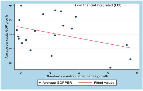
Further, this is confirmed by the scatter plot of GDP per capita growth with volatility. The figure for full sample of countries is presented in Figure 1(a,b). A negative growth–volatility relationship is seen across all the countries for both the measures of volatility, i.e. standard deviation of per capita GDP growth and standard deviation of output gap. But a positive relationship between growth and volatility among the industrial economies (Figure 2) is seen, whereas for developing countries the relationship is negative (Figure 3). It is also seen that the relationship between growth and volatility is strongly negative for LFI economies (Figure 5) and the same is positive for the HFI economies (Figure 4). Therefore, we may say that the poor countries are somewhat more volatile in nature compared to the developed ones.

Figure 1. (a) Full sample of countries. (b) Full sample of countries

(mean growth and SD of output growth)

Figure 1b. (continued)

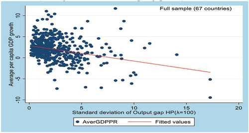
Figure 2. Industrial countries

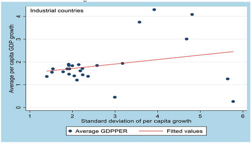
Figure 3. Developing countries

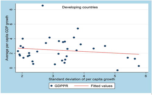
Figure 4. High financial integreted (HFI)

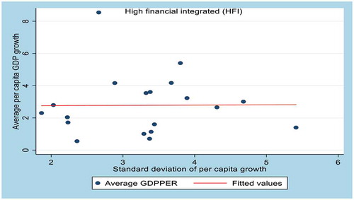
Figure 5. Low financial integreted (LFI)

Further, a decadal analysis of the macroeconomic fluctuations over the sample period is attempted. The results are presented in Table 2. It is found that the average output growth in the industrial economies has been declining over the four decades. Though, the output volatility declined in first three decades, it increased again in the fourth decade. This decline in macroeconomic fluctuations is also seen in the study by Stock and Watson (2002), in which they confirm that from 1970s to 2000s, the industrial countries witness steady decline in output volatility and steady rise in output growth rate. In the developing country sample both, HFI and LFI countries notice a decrease in average output growth in the decades of the 1980s and 1990s. The growth rebounds in 2000s and 2010s with an average increase of two points. Both the HFI and LFI economies experience high output volatility, which is more than its output growth in the 1980s and 1990s. It is found that there is substantial rise in volume of international trade and financial flows to the developing countries from the industrial economies during mid-1980s to 1990s (Kose et al., 2003a). Private capital also has moved from developed economies to developing nations between these periods. Further, the HFI and LFI ones show high average government consumption growth as well as high volatility in average government consumption compared to the industrial economies.

The results for average private consumption growth and volatility show a similar pattern for HFI and LFI countries. They have the highest average private consumption growth rate compared to industrial economics and at the same time these countries experience the highest volatility. Moreover, the LFI economies witness higher volatility, i.e. two times greater than its average growth followed by HFI and industrial countries. The industrial economies show the highest average private consumption growth and the lowest volatility in 1980s and 1990s. Towards the end of the 2010, the growth rate of private consumption for industrial countries decrease to 1.62. Overall, volatility decrease for all the three groups of the countries studied here.

The results for levels and volatility of investment growth reported in Table 2 also show that the average investment growth, increase for the industrial economies in the 1990s and 2000s, followed by a decline in 2010s. Coming to the developing countries average investment growth see a slowdown in the 1980s and an increase from the 1990s. Further, investment growth in HFI and LFI increase since 1990s. Interestingly, the volatility of investment growth also increases in 2000 for both LFI and industrial economies. But for HFI economies both investment growth and volatility decline.⁵

In case of import and export reported in Table 3, growth and volatility relationship differs across all the three groups of countries. Over the full sample period, the highest average export growth and lowest volatility are seen in HFI economies, followed by industrial economies and LFIs. The highest average import growth and highest volatility is seen in LFI economies, followed by HFI and industrial countries. During the 1990s, HFI countries experience the highest average export growth and lowest volatility in developing country group. Towards the end of 2010, LFI economies witness high level of average export growth with high volatility in the developing country group.

Table 3. Growth and volatility (Mean and standard deviation for selected macroeconomic variables)

Countries groups	Full sample 1978–2017	Decade				Full sample 1978–2017	Decade
		1978–1987	1988–1997	1998–2007	2008–2017		1978–1987	1988–1997	1998–2007	2008–2017
(5) Export Growth						Import Growth
Industrial Economies	5.18	5.11	7.11	5.26	2.90	5.01	4.42	6.83	6.07	2.74
Developing Economies*	5.49	5.81	6.50	6.25	3.53	4.91	2.43	6.88	6.10	4.23
HFI** Economies	588	5.63	7.38	7.17	2.87	5.59	3.46	9.38	6.42	3.11
LFI*** Economies	5.11	6.00	5.16	5.35	4.18	4.23	1.41	4.37	5.79	5.35
Export volatility						Import volatility
Industrial Economies	5.56	5.19	4.35	4.90	6.26	6.49	2.35	2.36	1.90	2.46
Developing Economies*	11.98	15.52	8.72	6.25	9.38	12.84	15.56	11.98	10.11	10.32
HFI** Economies	9.25	11.41	6.48	7.17	8.20	12.10	14.11	10.09	10.65	10.33
LFI*** Economies	14.72	19.63	10.96	5.35	10.57	13.57	17.02	13.87	9.56	10.30

*Developing economies (HFI+LFI) **HFI (High financial integrated) and *** LFI (Low financial integrated)

To further the growth-volatility analysis, cross-sectional regressions are run between output growth and its volatility in line with Ramey and Ramey (1995). The regression results are reported for the full sample of 67 countries, and sub samples of 27 industrial countries, 20 high financial integrated economies and 20 low financial integrated economies over the period of 1978–2017. The cross-sectional regression results with GDP per capita as dependent variable and output volatility as explanatory variable are presented in Tables 4 and 5.⁶ The estimated coefficient for the full sample yields a negative and significant association between economic growth and volatility implying one-standard deviation increase in macroeconomic volatility results in an average decline of 0.31% point of annual per-capita growth of the economy. It is also evident that countries with higher volatility in growth rates tend to have systematically lower growth rates⁷ (Figure 1(a,b)). In case of different country groups, the 27 industrial economies yield a positive coefficient of 0.23 but not significantly different from zero at 5% level. This is contrast to Ramey and Ramey (1995), where the relationship is found to be negative and significant for 24 OECD economies. One of the potential reasons for this difference could be that the positive association between output volatility and output growth among industrial economies might have become stronger over time. In case of developing country groups, the relationship between growth and volatility is negative and highly significant. Further, one standard deviation increase in output volatility leads to a decline of 0.5 percent in the growth rate. Coming to the HFI and LFI economies, the results indicate that HFI economies witness positive but insignificant relationship between economic growth and volatility. However, LFI economies show negative and statistically significant effect of output volatility on economic growth.

Table 4. Cross-section regression GDP per capita growth and volatility (1978–2017) (Volatility as standard deviation of output growth)

Independent variable	Full sample	Industrial Economies	Developing Economies	HFI Economies	LFI Economies
Constant	−3.03 (<.001) ***	−3.95 (0.01) **	−2.97 (0.002) ***	−3.59 (0.007) ***	−0.61 (0.64)
Volatility	−0.318 (0.005)***	0.232 (0.19)	−0.50 <.001***	−0.32 (0.16)	−0.45 (0.009)***
Average investment percentage of GDP	0.255 <.001***	0.15 (0.01)***	0.28 <.001***	0.34 <.001***	0.13 (0.04)**
Secondary Education (as human capital)	0.15 (0.2)	0.23 (0.03)**	0.19 (0.02)**	−0.20 (0.89)	0.31 (0.004)***
Initial per capita GDP	−0.0007 <.001***	−0.00022 (0.25)	−0.00001 <.001***	−0.000007 (0.09)*	−0.00011 (0.001)***
Number of observations	67	27	40	20	20
Adjusted R-squared	0.58	0.32	0.72	0.8	0.63

Notes: GDP per capita growth rate used as a dependent variable. All regressions run including intercept. Standard errors are presented in brackets are p-values and the character “*” “**” “***” indicates “10ʹ,”5ʹ,’1ʹ per cent level of significance.

Next, the cross-section models are augmented with additional control variables taken from growth literature. The possible control variables are investment to GDP ratio, initial log GDP per capita (to account for transitional convergence effect), initial human capital (to account the human capital investment). In addition to this, variables such as government consumption expenditure as % of GDP, trade openness index and indicator⁸ are also employed as control variables (Levine & Renelt, 1992; Barro & Lee., 2001; Aizenman and Marion, 1999). The results with the full set of control variables presented in Tables 6 and 7 yield a negative and statistically significant coefficient of −0.31 for the full sample. In the case of developing country sample, the coefficient is −0.39 and statistically significant. In both the cases, the inclusion of full set of controls results in lower negative coefficient of output volatility. This implies that the significant effect of additional control variables on growth-volatility relationship.

Table 5. Cross-section regression GDP per capita growth and volatility (1978–2017) (Volatility as standard deviation of output gap HP λ-100)

Independent variable	Full sample	Industrial Economies	Developing Economies	HFI Economies	LFI Economies
Constant	−3.13 <.001***	−3.92 (0.01)**	−3.18 (0.001)***	−3.78 (0.005)***	−0.82 (0.54)
Volatility	−0.31 (0.01)**	0.32 (0.14)	−0.57 (0.001)***	−0.33 (0.24)	−0.51 (0.02)**
Average investment percentage of GDP	0.25 <.001***	0.15 (0.008)***	0.28 <.001***	0.33 <.001***	0.14 (0.05)**
Secondary Education (as human capital)	0.14 (0.02)**	0.21 (0.03)**	0.16 (0.05)**	−0.04 (0.74)	0.28 (0.01)**
Initial per capita GDP	−0.00006 <.001***	−0.00019 (0.37)	−0.00009 (0.001)***	−0.000006 (0.12)	−0.0001 (0.003)***
Number of observations	67	27	40	20	20
Adjusted R-squared	0.57	0.33	0.71	0.79	0.60

Notes: GDP per capita growth rate used as a dependent variable. All regressions run including intercept. Standard errors are presented in brackets are p-values and the character “*” “**” “***” indicates “10ʹ,”5ʹ,’1ʹ per cent level of significant.

Table 6. Cross-section regression GDP per capita growth and its volatility (1978–2017): (volatility as SD of output growth) (Including policy variables and variable)

Independent variable	Full sample	Industrial Economies	Developing Economies	HFI Economies	LFI Economies
Constant	−2.33 (0.02)**	−6.73 (0.003)***	−1.64 (0.15)	−1.89 (0.44)	−1.02 (0.49)
Volatility	−0.31 (0.01)**	0.12 (0.47)	−0.39 (0.006)***	−0.28 (0.31)	−0.37 (0.02)**
Average investment percentage of GDP	0.22 <.001**	0.05 (0.36)	0.25 <.001**	0.31 (0.001)**	0.13 (0.05)**
Secondary Education (as human capital)	0.16 (0.01)**	0.23 (0.01)**	0.17 (0.04)**	−0.03 (0.87)	0.26 (0.01)**
Initial per capita GDP	−0.0006 <.001***	−0.00003 (0.07)*	−0.00008 (0.01)**	−0.000001 (0.50)	−0.00011 (0.07)*
Trade openness (in log)	0.06 (0.78)	0.60 (0.02)**	−0.39 (0.25)	−0.67 (0.26)	0.38 (0.45)
(Private credit % of GDP)	0.23 (0.41)	0.82 (0.03)**	0.54 (0.14)	0.68 (0.52)	0.16 (0.7)
Government expenditure (% of GDP)	−0.08 (0.005)***	−0.20 (0.51)	−0.10 (0.02)**	−0.80 (0.65)	−0.12 (0.01)**
Number of observations	67	27	40	20	20
Adjusted R-squared	0.66	0.55	0.76	0.76	0.78

Notes: GDP per capita growth rate used as a dependent variable. All regressions run including intercept. Dummy variables taken for country group developed HFI

and LFI. Standard errors are presented in brackets are p-values and the character “*” “**” “***” indicates “10ʹ,”5ʹ,’1ʹ per cent level of significance.

Among the control variables, average investment as % of GDP is positive and highly significant, initial per capita income is negative and significant and human capital is positive but insignificant. The convergence is found to be slow in view of the low coefficient of initial per capita income. Similarly, the coefficients of human capital indicate a weak positive association. The policy variable, government consumption expenditure shows negative and significant impact on growth for full sample and developing countries. But for industrial economies, it is negative and insignificant. Government consumption expenditure is negative and statistically significant for LFI economies. This may be because in developing countries most of the government expenditure may have been on unproductive projects. The trade openness index shows a positive and significant relationship between trade and economic growth. But the relationship is not clear in case of developing countries. The reason may be import of more capital goods, export of primary goods and insufficient trade share to balance the budget in case of these countries(Kose et al., 2003a). The indicator bears the expected sign implying that works smoothly in industrial economies compared to the developing economies (the coefficients are positive but not significant), as shown in Levine and Renelt (1992), Ramey and Ramey (1995), and Fatás and Mihov (2003) hypotheses. The regressions, when re-estimated using volatility of output gap do not show any difference compared to the regressions with standard deviation of output-measuring volatility.

Next, the panel regression results are presented considering the change of growth–volatility relationship over time within a country group. Following some of the past studies, five-year non-overlapping annual averages of the variables, i.e. maximum of eight observations for each country are used in the panel data estimation. The panel data set up accounts for both time-invariant country-specific effects and country-invariant time-specific effects. The obvious advantage of panel data lies in eliminating omitted-variable bias as well as getting more degrees of freedom and more efficiency in estimation. The following model is estimated for three different country groups.

(5) $\mathrm{G}{\mathrm{r}}_{\mathrm{i}\mathrm{t}}={\beta }_0+{\beta }_1\mathrm{v}\mathrm{o}{\mathrm{l}}_{\mathrm{i}\mathrm{t}}+{\beta }_2{\mathrm{X}}_{\mathrm{i}\mathrm{t}}+{\mathrm{\partial }}_{\mathrm{i}}+{\gamma }_{\mathrm{t}}+{\epsilon }_{\mathrm{i}\mathrm{t}}$(5)

where ‘i’ denotes country and “t” denotes time, $\mathrm{\partial }$_i stands for unobserved country-specific effect,$\gamma$_t is time-fixed effect and $\epsilon$_it is the error term. Hausman’s (1978) test is used to choose between fixed and random effect specification. The null hypothesis in Hausman’s test is that the chosen model is random effects against the alternative of fixed effects. The approach basically tests whether the errors u_i are correlated with the regressors. For completeness sake, pooled, fixed effect and random effect regressions are run and the best model is selected based on the Hausman’s test. The results from the pooled, fixed, and random effect regressions presented in Table 8, show a statistically significant negative contemporaneous relationship between economic growth and output volatility for the full sample of 67 countries. The above regressions are then augmented with full set of control variables. Three out of six control variables namely log of initial income, investment as a percentage of GDP and government expenditure as percentage of GDP are statistically significant with theoretically expected signs across the pooled, fixed, and random effects regressions. It may be noted that among the other control variables private credit as percentage of GDP and human capital bear-mixed signs and significance, yielding ambiguous relationship with economic growth across all the three specifications. Hence, the association between growth and volatility become stronger once we include a set of control variables. These results are like results obtained in some of the previous studies by Ramey and Ramey (1995), Levine and Renelt (1992), and Kose et al. (2006).

Table 7. Cross-section regression GDP per capita growth and its volatility (1978–2017): (volatility as SD output gap) (Including policy variables and financial depth variable)

Independent variable	Full sample	Industrial Economies	Developing Economies	HFI Economies	LFI Economies
Constant	−2.31 (0.02)**	−0.68 (0.002)***	−1.76 (0.13)	−2.20 (0.36)	−1.03 (0.53)
Volatility	−0.30 (0.03)**	0.19 (0.37)	−0.41 (0.02)**	−0.24 (0.45)	−0.38 (0.08)*
Average investment percentage of GDP	0.22 <.001***	0.05 (0.34)	0.25 <.001***	0.31 (0.001)***	0.14 (0.05)**
Secondary Education (as human capital)	0.16 (0.02)**	0.21 (0.01)**	0.15 (0.08)*	−0.003 (0.98)	0.26 (0.03)**
Initial per capita GDP	−0.0006 <.001***	−0.00027 (0.09)*	−0.00006 (0.03)**	−0.000005 (−0.53)	−0.00006 (0.01)**
Trade openness (in log)	0.02 (0.91)	0.56 (0.04)**	−0.41 (0.25)	−0.69 (0.28)	0.34 (0.55)
(Private credit % of GDP)	0.23 (0.43)	0.87 (0.02)**	0.51 (0.20)	0.56 (0.56)	0.05 (0.90)
Government expenditure (% of GDP)	−0.08 (0.006)***	−0.17 (0.59)	−0.10 (0.03)**	−0.06 (0.74)	−0.12 (0.01)**
Number of observations	67	27	40	20	20
Adjusted R-squared	0.60	0.55	0.74	0.77	0.70

Notes: GDP per capita growth rate used as a dependent variable. All regressions run including intercept. Dummy variables taken for country group developed HFI

and LFI. Standard errors are presented in brackets are p-values and the character “*” “**” “***” indicates “10ʹ,”5ʹ,’1ʹ per cent level of significance.

Table 8. Panel regression (fixed vs. random effect) GDP per capita growth and volatility (1978–2017)

Independent variable	Pooled OLS Full sample	Fixed effect Full sample	Random Full sample
Constant	4.80 (<.001***)	11.22 (0.002)***	4.82 (<.001***)
Volatility	−0.28 (<.001***)	−0.29 (<.001***)	−0.28 (<.001***)
Average investment percentage of GDP	0.16 (<.001***)	0.13 (<.001***)	0.15 (<.001***)
Secondary Education (as human capital)	0.04 (0.44)	−0.18 (0.07)*	−0.03 (0.63)
Initial per capita GDP	−0.55 (<.001***)	−0.79 (0.10)*	−0.40 (0.008)***
Trade openness (in log)	0.006 (<.001***)	0.009 (0.04)**	−0.005 (0.003)***
Financial depth (Private credit % of GDP)	0.22 (0.17)	−0.17 (0.51)	0.09 (0.63)
Government expenditure (% of GDP)	−0.07 (0.001)***	−0.13 (0.001)***	−0.08 (0.001)***
Number of observations	536	536	536
Adjusted R-squared	0.34	0.17	0.34
Hausman test			0.0000***

Notes: GDP per capita growth rate used as a dependent variable. All regressions run including intercept. Dummy variables taken

For country group developed HFI and LFI. Standard errors are presented in brackets are p-values and the character “*” “**” “***”

Indicates “10ʹ,”5ʹ,’1ʹ per cent level of significance.

Further, panel regressions are estimated for the full sample as well as for the four country groups i.e. developing, industrial, HFI, and LFI. The results are reported in Table 9, where Hausman’s test favours the fixed effect model for full sample, developing and industrial countries. The output volatility has positive and significant effect on economic growth for the full sample. Thus, higher the growth rate, higher is the output volatility. To be precise, one standard deviation increase in output volatility leads to 0.29% increase in average GDP growth the full sample. For the developing and industrial countries, the coefficients are −0.31 and 0.26. These results are like the findings of Kormendi and Meguire (1985), and Grier and Tullock (1989), where higher standard deviation of GDP growth is associated with greater economic growth, due to aggregate trade-off between risk and returns. Similarly, the coefficient of volatility bears negative sign and is statistically significant for developing economies. However, in case of industrial countries, one standard deviation increase in volatility leads to 0.26% increase in economic growth.

Table 9. Fixed-effect estimations of GDP per capita growth and volatility (1978–2017)

Independent variable	Full sample	Industrial	Developing
Constant	11.22 (0.002)***	7.84 (0.34)	12.01 (0.003)***
Volatility	0.29 (<.001***)	0.26 (0.001)***	−0.31 (<.001***)
Average investment percentage of GDP	0.13 (<.001***)	0.02 (0.51)	0.15 (<.001***)
Secondary Education (as human capital)	−0.18 (0.07)*	−0.29 (0.04)**	0.11 (0.42)
Initial per capita GDP	−0.79 (0.10)*	0.62 (0.47)	−1.16 (0.05)**
Trade openness (in log)	0.009 (0.04)**	0.002 (0.62)	−0.10 (0.19)
Financial depth (Private credit % of GDP)	−0.17 (0.51)	−0.50 (0.12)	−0.14 (0.72)
Government expenditure (% of GDP)	−0.13 (0.001)***	−0.38 <.001***	−0.08 (0.11)
Inflation	−0.01 (<.001***)	0.01 (0.11)	−0.02 (<.001***)
Number of observations	536	216	320
Adjusted R-squared	0.17	0.15	0.25
Hausman test	0.0000***	0.0000***	0.0001***

Notes: GDP per capita growth rate used as a dependent variable. All regressions run including intercept. Dummy variables taken

for country group developed HFIs and LFIs. Standard errors are presented in brackets are p-values and the character “*” “**” “***”

Indicates “10ʹ,”5ʹ,’1ʹ per cent level of significance.

After including control variables as mentioned above one finds that the estimated coefficient on initial per capita GDP is negative as expected for the developing countries. Thus, a significant convergence effect is confirmed for developing economies. One percent increase in initial per capita GDP leads to 1.16% decline in economic growth. Further, the coefficients of trade openness show negative but insignificant effect on growth. Among other control variables, government expenditure as percentage of GDP is negative for both developing and industrial country groups. But the effect is significant only for industrial counties. The reasons underlying such results may be that higher taxes induce more government spending. But inefficient allocation of resources and unexpected economic fluctuations can reduce the output growth level (Kormendi & Meguire, 1985). Inflation has significant and negative effect on economic growth for developing countries as expected. The evidence goes against the Mundell-Tobin hypothesis.⁹ But it supports that of Stockman’s (1981), i.e. at higher rates of inflation, money being relatively costly to hold, net return from investment becomes lower. As a result, steady state capital stock also declines due to lower investment. This implies reduction in investment, lower capital stock and lower economic growth (Kormendi & Meguire, 1985). Finally, the proxy of i.e. private credit as percentage of GDP shows negative but insignificant relationship between economic growth and. Hence, the above results confirm that developing countries are highly volatile in nature compared to industrial countries. It may be noted that the industrial countries are highly capable in stabilising their economy compared to the developing ones. The results in Table 10 with random effect regressions as favoured by the Hausman test for HFI and LFI yield that volatility coefficients are negative and significant with all the control variables. However, the HFI yield coefficients of higher magnitude compared to the LFI. The coefficients of control variables vary dramatically across the two subsamples. Investment as percentage of GDP explains economic growth better for both the country groups. While the government expenditure percentage of GDP and Inflation is negative and significant for HFI, the same is insignificant for LFI. The coefficients on Private credit percentage of GDP are positive and significant only for HFI countries. These results are consistent with Levine and Renelt (1992) and Kose et al. (2003a), and Easterly and Stiglitz (2000).

Table 10. Random-effect estimations of GDP per capita growth and volatility (1978–2017)

Independent variable	Low financial integrated (LFI)	High financial integrated (HFI)
Constant	6.18 (0.002)***	5.82 (0.03)***
Volatility	−0.19 (0.01)**	−0.53 (<.001***)
Average investment percentage of GDP	0.17 (<.001***)	0.13 (<.001***)
Secondary Education (as human capital)	0.18 (0.10)*	−0.19 (0.16)
Initial per capita GDP	−0.97 (0.004)***	−0.41 (0.18)
Trade openness (in log)	0.01 (0.13)	0.001 (0.87)
Financial depth (Private credit % of GDP)	0.02 (0.93)	0.75 (0.09)*
Government expenditure (% of GDP)	0.005 (0.93)	−0.14 (0.006)***
Inflation	−0.01 (0.22)	−0.009 (0.02)**
Number of observations	160	160
Adjusted R-squared	0.34	0.52
Hausman test	0.073	0.053

Notes: GDP per capita growth rate used as a dependent variable. All regressions run including intercept. Dummy variables taken

for country group developed HFIs and LFIs. Standard errors are presented in brackets are p-values and the character “*” “**”

“***” indicates “10ʹ,”5ʹ,’1ʹ per cent level of significance.

4. Conclusion

This paper attempts a re-examination of the relationship between output volatility as a proxy of macroeconomic volatility and economic growth for a select sample of 67 countries (40 developing and 27 industrial counties) over an annual data set spanning, 1978 to 2017. The main conclusion of this paper is that output volatility has negative effect on economic growth, and it is confirmed by both cross-section and panel regression results. Further, the negative output volatility and growth relationship is found to be stronger for the developing countries. These results support the theoretical insights given by Martin and Rogers (2000), Fatás and Mihov (2003), Hnatkovska,, & Norman, L. (2003), and Loayza et al. (2007). For industrial countries, we find a positive and significant relationship between growth-volatility, which contrasts with Ramey and Ramey (1995), but resonates findings of Kormendi and Meguire (1985), Grier and Tullock (1989), Caporale and McKiernan (1998), and Ramey and Ramey (1995) find negative and significant effect of output volatility on growth for 24 OECD countries and the underlying reason may be different time period of the study. The results regarding the control variables in this study are consistent with growth theory, except human capital and trade openness. As a robustness check, we estimate the models for HFI and LFI groups separately. We find a negative and significant relationship between output volatility and economic growth. This might be due to the intermediate stage of financial market development or maybe due to poor institutional setups resulting in poor management of unpredictable shocks. Overall, the results suggest a bit of ambiguity except the clear negative relationship found for developing countries. The results of different samples of HFIs and LFIs speak of the role financial integration plays in defining growth volatility relationship. However, further research in future may focus on the channels causing such negative relationship in the presence of financial integration. To substantiate the role of financial integration in bringing out the changing nature of volatility growth relationship, one may examine the impact of different types of financial flows.

Additional information

Funding

The authors received no direct funding for this research.

Notes on contributors

Y N Raju

Y N Raju is a Rajiv Gandhi National Fellow pursuing his final year PhD in the School of Economics, University of Hyderabad. He is working on empirical aspects of trade and financial integration, volatility, and Growth.

Debashis Acharya

Debashis Acharya is a Professor of Economics in University of Hyderabad’s School of Economics. He has published in the areas of Macro-monetary economics, Financial economics and Development economics in international and national referred journals. Some of these include European Journal of Operational Research, The Australian Economic Review, Global Business Review, Journal of Financial Economic and Policy, Journal of Quantitative Economics, Economic Change and Restructuring. Macroeconomics and Finance in Emerging Market Economies, South Asia Economic Journal, Economic and Political Weekly etc. He is currently serving as Associate Editor in Indian Economic Journal and Asia- Pacific Journal of Regional Science, Springer.

Notes

1. Schumpeter’s (1939) idea of “creative destruction”

2. Redux model of Maurice and Rogoff (1995)

3. The HFI (high financial integrated) countries are also called “emerging markets” according to the methodology used by MSCI GIMI (global investable markets index). Next LFI (less financial integrated) countries are called as “Frontier market”. The methodology used to construct the MSCI Frontier Markets Indexes is similar, but not identical, to the construction of the indexes for Developed and Emerging Markets. One of the prime differences is that the Frontier Markets are divided into size (Large, Small) and liquidity (Average, Low, and Very Low) categories (MSCI Global Investable Market Indexes Methodology, 2017).

4. All conditional variables include period dummies to control for time-varying factors and country-specific dummies to arrest the effect of structural variables that does not change over time.

5. Kose et al. (2003a) find that industrial countries have high investment growth in 1980s and 1990s compare to HFIs and LFIs with less volatility.

6. The GDP per capita and its volatility are averages over 1978–2017.

7. We find the similar results when we used standard deviation of output gap as volatility.

8. We dropped population growth and inflation in this due to large outliers

9. Mundell (1963) and Tobin (1965) argued that higher inflation leads to shifts away from real money balance to real capital assets, therefore higher investment and higher economic growth.

Appendix A

Table A1. List of sample countries (67)

Industrial countries	High Financial Integrated (HFI)	Low Financial Integrated (LFI)
Australia	Chile	Malta
Belgium	Greece	Jordan
Canada	Korea, Rep.	Mauritius
Denmark	Brazil	Sri Lanka
Finland	China	Bangladesh
France	Colombia	Kenya
Germany	Malaysia	Morocco
Hong Kong SAR, China	Mexico	Senegal
Ireland	Peru	Tunisia
Israel	South Africa	Sierra Leone
Italy	Thailand	Niger
Japan	Turkey	Togo
Netherlands	Egypt, Arab Rep.	Belize
New Zealand	India	Benin
Norway	Indonesia	Bolivia
Portugal	Pakistan	Cameroon
Singapore	Philippines	Congo, Rep.
Spain	El Salvador	Gabon
Sweden	Gambia	Malawi
Switzerland	Iran, Islamic Rep.	Central African Republic
United Kingdom
United States
Panama
Jamaica
Uruguay
Luxembourg
Fiji

References

- Abel Andrew, B. (1983). Optimal investment under uncertainty. American Economic Review, 73, 228–23.
- Aghion, P., Banerjee, A., & Piketty, T. (1999). Dualism and macroeconomic volatility. Quarterly Journal of Economics, 114(4), 1359–1397. https://doi.org/10.1162/003355399556296
- Aghion, P., & Saint-Paul, G. (1998). Virtues of bad time’s interaction between productivity growth and economic fluctuations. Macroeconomic Dynamics, 2(3), 322–344. doi:10.1017/S1365100598008025
- Aizenman, J., & Marion, N. (1993). Policy uncertainty, persistence, and growth. Review of International Economics, 1(2), 145–163. https://doi.org/10.1111/j.1467-9396.1993.tb00012.x
- Aizenman, J., & Marion, N. (1999). Volatility and investment: Interpreting evidence from developing countries. Economica, 66(262), 157–179. https://doi.org/10.1111/1468-0335.00163
- Barro, R. J., & Lee., J. W. (2001). International data on educational attainment: Updates and Implications. Oxford Economic Papers, 53(3), 541–563. https://doi.org/10.1093/oep/53.3.541
- Bugamelli, M., & Paterno, F. (2009). Output growth volatility and remittances. Economica, 78(311), 480–500. https://doi.org/10.1111/j.1468-0335.2009.00838.x
- Caballero, R. J. (1991). On the sign of the investment-uncertainty relationship. The American Economic Review, 81(1), 279–288
- Caporale, T., & McKiernan, B. (1996). The relationship between output variability and growth: Evidence from post war UK data. Scottish Journal of Political Economy, 43(2), 229–236. https://doi.org/10.1111/j.1467-9485.1996.tb00675.x
- Caporale, T., & McKiernan, B. (1998). The fischer–black hypothesis: Some time-series evidence. Southern Economic Journal, 64(3), 765–771. https://doi.org/10.2307/1060792
- Easterly, W., Islam, R., & Stiglitz, J. E. (2000). Shaken and stirred: Explaining growth volatility. In B. Pleskovic and J. E. Stiglitz (eds), Annual world bank conference on development economics 2000. Washington DC: World Bank
- Fatas, A. (2002). The effects of business cycles on growth. In N. Loayza & R. Soto (Eds.), Economic growth: Sources, trends and cycles (pp. 191-219). Central Bank of Chile.
- Fatás, A., & Mihov, I. (2003). The case for restricting fiscal policy discretion. The Quarterly Journal of Economics, 118(4), 1419–1447. https://doi.org/10.1162/003355303322552838
- Gavin, M., & Hausmann, R. (1995). Overcoming Volatility in Latin America. Washington, DC: Inter-American Development Bank.
- Grier, K., & Tullock, G. (1989). An empirical analysis of cross-national economic growth, 1951-80. Journal of Monetary Economics, 24(2), 259–276. https://doi.org/10.1016/0304-3932(89)90006-8
- Grier, K. B., & Perry, M. J. (2000). The effects of real and nominal uncertainty on inflation and output growth: some garch-m evidence. Journal of Applied Econometrics, 15(1), 45–58. doi:10.1002/(ISSN)1099-1255
- Grinols, E. L., & Turnovsky, S. J. (1994). Exchange rate determination and asset prices in a stochastic small open economy. Journal of International Economics, 36(1–2), 75–97. https://doi.org/10.1016/0022-1996(94)90058-2
- Grinols, E. L., & Turnovsky, S. J. (1998). Risk, optimal government finance and monetary policies in a growing economy. Economica, 65(259), 401–427. https://doi.org/10.1111/1468-0335.00136
- Hausman, J. A. (1978). Specification Tests in Econometrics. Econometrica, 46(6), 1251–1271. https://doi.org/10.2307/1913827
- Hnatkovska, V. (2005). Appendix. In J. Azeinman & B. Pinto (Eds.), Managing economic volatility and crises (pp. 65-100). Cambridge University Press.
- Hnatkovska, V., & Norman, L. 2003, Volatility and Growth. Policy Research Working Paper Series 3184, 1-40. The World Bank.
- Hodrick, R., & Prescott, E. (1997). Postwar US business cycles: An empirical investigation. Journal of Money, Credit and Banking, 29(1), 1–16. https://doi.org/10.2307/2953682
- Kormendi, R., & Meguire, P. (1985). Macroeconomic determinants of growth: Cross-country evidence. Journal of Monetary Economics, 16(2), 141–163. https://doi.org/10.1016/0304-3932(85)90027-3
- Kose, M. A., Prasad, E. S., & Terrones, M. E. (2003a). Financial integration and macroeconomic volatility. IMF Staff Papers, 50, 119–142. https://www.jstor.org/stable/pdf/4149918.pdf
- Kose, M. A., Prasad, E. S., & Terrones, M. E. (2006). How do trade and financial integration affect the relationship between growth and volatility?. Journal of international Economics, 69(1), 176–202. doi:10.1016/j.jinteco.2005.05.009
- Levine, R., & Renelt, D. (1992). A sensitivity analysis of cross-country growth regressions. American Economic Review, 82(4), 942–963. https://www.jstor.org/stable/pdf/2117352.pdf
- Loayza, N. V., Ranciere, R., Servén, L., & Ventura, J. (2007). Macroeconomic volatility and welfare in developing countries: An introduction. The World Bank Economic Review, 21(3), :343–357. https://doi.org/10.1093/wber/lhm017
- Martin, P., & Rogers, C. A. (2000). Long-term growth and short-term economic instability. European Economic Review, 44(2), 359–381. https://doi.org/10.1016/S0014-2921(98)00073-7
- Maurice, O. (1994). Risk-taking, global diversification and growth. American Economic Review, 84, 1310–1329.
- Maurice, O., & Rogoff, K. (1995). Exchange rate dynamics redux (NBER Working Paper No. 4693. National Bureau of Economic Research. https://www.nber.org/papers/w4093.pdf
- Mendoza, E. G. (1994). The robustness of macroeconomic indicators of capital mobility. In L. Leiderman & A. Razin (Eds.), Capital mobility: The impact on consumption, investment, and growth (pp. 83–111). Cambridge University Press.
- MSCI Global Investable Market Indexes Methodology. (2017). 86–100. New York, NY: Morgan Stanley Capital International.
- Ramey, G., & Ramey, V. A. 1991. Technology commitment and the cost economic fluctuations (NBER Working Paper 3755). National Bureau of Economic Research.
- Ramey, G., & Ramey, V. A. (1995). Cross-country evidence on the link between volatility and growth. American Economic Review, 85(5), 1138–1151.
- Schumpeter, J. A. (1939). Business cycles. McGraw-Hill.
- Senay, O. (1998). The effects of goods and financial market integration on macroeconomic volatility. The Manchester School, 66(S), 39–61.
- Stock, J. H., & Watson, M. W. (2002). Has the business cycle changed and why? NBER macroeconomics annual, 17, 159–218 doi:10.1086/ma.17.3585284
- Sutherland, A. (1996). Financial market integration and macroeconomic volatility. The Scandinavian Journal of Economics, 521–539 4 98. doi:10.2307/3440882
- Tobin, J. (1965). Money and economic growth. Econometrica: Journal of the Econometric Society, 33(4) 671–684. doi:10.2307/1910352
- Turnovsky Stephen, J., & Chattopadhyay, P. (2003). Volatility and growth in developing economies: Some numerical results and empirical evidence. Journal of International Economics, 52(2), 267–295. https://doi.org/10.1016/S0022-1996(02)00016-8
- Wolf, H. (2005). Volatility: Definitions and consequences. In J. Azeinman & B. Pinto (Eds.), Managing economic volatility and crises (pp. 45-64). Cambridge University Press.