
 ?Mathematical formulae have been encoded as MathML and are displayed in this HTML version using MathJax in order to improve their display. Uncheck the box to turn MathJax off. This feature requires Javascript. Click on a formula to zoom.
Abstract
Findings from previous studies indicate that the long-run stationarity of the real exchange rate in different time horizons remains unclear. In order to shed light on this problem, we have adopted a new method which is widely used to analyze signals, the so-called wavelet transformation. This paper uses monthly data of the consumer price indices (CPI) and nominal exchange rates for six ASEAN countries for the 1998–2019 period. The unobserved component method is used to remove the seasonality and cyclicity of the CPI. Then, the real exchange rates are calculated. We use the unit root tests and wavelet transformation to verify if the purchasing power parity (PPP) holds in the long run in different time horizons. Key findings from the paper are as follows. First, the mean-reverting pattern of real exchange rate recurs itself for the period longer than 5 years. Second, the variation around trend using wavelet methodology can be used as a reliable indicator for future movements of the real exchange rate. Third, the high volatility of the exchange rate in the short run may be induced by arbitrage activities. Implications have emerged based on these findings for policymakers and investors in relation to the behaviour of the real exchange rate.
PUBLIC INTEREST STATEMENT
The real exchange rate is driven by many factors. We are interested in its long-run dynamics which are affected by activities in relation to high-frequency changes in price. This study is conducted to investigate the validity of the purchasing power parity (PPP) in the long-run using the multi-resolution analysis (MRA). We argue that the validity of the PPP depends mostly on the definition of a long run and its measurement.
In this paper, we use a wavelet decomposition, which is widely used in digital and signal processing, and unobserved component analysis for exploring the real exchange rate patterns of the ASEAN countries using monthly data for the period from 1998 to 2019. Findings from our paper indicate that the mean-reverting pattern of the real exchange rate recurs itself for the period longer than 5 years. In addition, the MRA method provides the central banks and the governments with a convincing pattern of real exchange rate movements in the future for policy purposes.
1. Introduction
The validation of the purchasing power parity (PPP) is widely discussed in many academic papers. The law of one price (LOP) indicates that the value of any common good should be the same when any pair of currency is taken into consideration. Many classical economists refer to this idea as the real covariate (Patinkin, Citation1965). The PPP and its validation are distinctive phenomena of a classical dichotomy, which has attracted great attention from academics. An agreement has been achieved on the long-run validity of the PPP, while its short-run dynamics remain unclear (Salehizadeh & Taylor, Citation1999). This idea resounds with the efficient market hypothesis (EMH), which discusses a long-run market equilibrium. The short-run dynamic is a process of an un-correlated successive move (Malkiel, Citation2003). Unfortunately, the consensus has not been reached. The reason for this disagreement is mostly caused by the limited availability of historical data and limited methodologies in analyzing time series data.
Many previous studies have acknowledged that the long-run equilibrium of real exchange rate is a combination of many stationary processes. This is considered as the prerequisite for the long-run holds of the PPP. This primary condition is much alike to constitute the long-run stationarity of the efficient market hypothesis (EMH), which states that the price exploitation of any financial assets includes many random processes. In turn, the price discovery process is a set of the Brownian motion and white noise which captures the change in returns and is successively uncorrelated in different time horizons. This means that the price cannot be easily deduced just by gathering past information and today’s price, which is then considered the best reflection of tomorrow price. Additionally, the effect of one-lagged observation on exchange rate prediction is significant and long-lasting.
The perspective of the investment horizon differs among economic entities. Some investors who are only excited in the short-run movement in price prefer intraday trade for exploiting capital gains. International hedging managers prefer using currency market or the capital market as a tool for minimizing unsystematic risk. Policymakers who are very interested in the long-run dynamics of the real exchange rate consider using financial instruments as a tool for economic stabilization. By conducting large and infrequent trade volume, market makers act as a catalyst for providing a medium and long-term steady growth through keeping inflation bounce in a pre-determined range. In comparison, individual investors, commercial banks, mutual fund managers utilize smaller trade volume. However, they trade more frequently than the market makers. Exploiting market defections and short-run incremental change in returns are the main objectives which these investors aim to do. In sum, the perspectives of different investment time horizons vary significantly among financial market participants, and their perspectives are reflected by their interests and actions. Due to the participation of diverse economic entities and their investment time scale, what we observed from historical recorded price is a combination of low, medium- and high-frequency changes in price level corresponding to the real exchange rate structure. Because of the real exchange rate is driven by many factors, we are only interested in its long-run dynamics which are shrouded by activities with respect to high-frequency changes in price. As such, an appropriate answer for the validation of the PPP depends mostly on how we define long run and how we measure it, for example, by a number of days, months or years. The novelty of our study is summarized as follows. First, existing methods are powerless in the provision of the specific time horizon at which the validity of the PPP hypothesis is confirmed. Previous studies also insufficiently provide empirical evidence which supports the mean-reversion of the real exchange rate (Adler & Lehmann, Citation1983; Roll, Citation1979). There is no attempt in utilizing wavelet decomposition and unobserved component analysis for exploring the real exchange rate pattern of the Asian countries (see for example, Baqaee (Citation2010) for New Zealand inflation rate; Vo and Vo (Citation2019b) for six pair of the exchange rate against the dollar). For that reason, we use wavelet analysis which is widely used in digital and signal processing. Second, we also make use of the multi-resolution analysis for the purpose of the projection of the real exchange rates. Our results confirm the usefulness of the approach for policymakers in formulating and implementing future monetary policies.
The paper is structured as follows. Following this introduction, Section 2 discusses relevant literature review. Next, the wavelet decomposition in analyzing time series is discussed in section 3. Section 4 presents the analyses on the validity of the PPP and our predictions for real exchange rates, followed by the conclusions in section 5.
2. Literature review
The purchasing power parity (PPP) hypothesis represents the process which comprises many price amendments. These price adjustments are deemed to be the consequence of exploiting international arbitrage. The arbitrage activities indirectly happen to rectify the price misalignments and cause real exchange rate mean-reverting (Vo and Vo, Citation2019b). Previous papers were conducted to examine real exchange rate dynamics. Using the augmented Dicky Fuller test and co-integration test, Salehizadeh and Taylor (Citation1999) demonstrate that the real exchange rate is misdirected from the true value after several years. They put great efforts into stylizing two-scale analyses—the short run and the long run. Their findings demonstrate that the real exchange rates are not affected by its nominal values. In contrast, other studies do not advocate the validity of the real exchange rate in the long run. Devoting to the idea, Engel and Roger (Citation1996) argue that the PPP is not consistent among different types of goods. They highlight the adverse impact of borderlines for rendering the price misalignment between different markets. Knetter (Citation1994) consider the difference in the price of goods is characterized by its transportation, insurance premium and level of trade liberalization.
The violation of the PPP, in the long run, can be attributed to market defections. In turn, individual investors might “overreact” to an upswing and downswing of exchange rates which might deflect its value away from the true value. De Bondt and Thaler (Citation1985) investigate the overreaction from historical events. The authors find that investors are sensitive to unforeseen and adverse information. Conventional tests such as stationarity and co-integration tests are widely applied in previous studies to examine the stationarity of the real exchange rate. Despite the presence of different stationary tests, the null hypothesis of those tests, time-series is non-stationary given by a sample period, is quite similar. Meanwhile, the null hypothesis should not be rejected unless the PPP’s validation is violated. If the null hypothesis cannot be rejected, then the PPP is successively uncorrelated or characterized by the Brownian motions.
The lack of precision of those tests is discussed. The augmented Dickey–Fuller (ADF) or Phillip-Perron (PP) tests fail to capture the exact order of integration, especially the first order and close to the first order. Another method for unit root testing is the KPSS test which was developed and first presented by Kwiatkowski et al. (Citation1992). The KPSS test is more powerful than the ADF and PP tests since it includes the stationarity around trend in its null hypothesis. Moreover, the stationarity of any time series is not necessary to be presented around a constant mean, but it can embody in an accelerating mean.
A stationary series in a classical econometric definition is an untransformed series whose mean, covariance and others are considered unchanged with respect to time variation. Practically, an absence of unit root is not characterized for a non-stationarity. A time series comprises an incremental mean over time, and “white” disturbance can also constitute a stationary process. Many econometricians consider this idea as a long-range dependency, meaning that the time series demonstrates a long memory. Granger and Joyeux (Citation1980) define a time series characterized by a long-range dependent process which will slowly have been decaying an autocorrelation function (ACF) instead of rapidly falling to 0. We can only confirm stationarity of any time series after deflating trend and correcting for its seasonality and cyclicity. Many techniques have been developed so far to address the confusion in the definitions of the so-called stationary series. Fractional Difference Process (FDP) defines a time series which have the order of integration at lag
if its ACF satisfies the following condition:
where
stands for the ACF function of obtained time series at lag
and constant term
. Hosking (Citation1981) when developing the Auto Regression Fractional Integration Model (ARFIMA) mentions that
in ARFIMA (0,
,0) is not necessarily an integer number and a time series is mean reverting even when
. Another method for measuring the long-run dependency of a given time series is Hurst exponent/coefficient, which is widely accepted and applicable in quantifying the long-term trend (mean-reversion) of any time process. Researchers consider Hurst exponent as a criterion for identifying the extent to which the stochastic process is dependent on its past value.
Hurst exponent was originally utilized in hydrology for determining optimal dam size for Nile’s river (Hurst, Citation1951). In order to gratitude the enormous contribution, the letter by which denotes the extent of long-dependency of a stochastic process is defined by its asymptotic behaviours over a rescaled range through
obtained observations (Qian et al., Citation2004). When
approach indefinite, the Hurst exponent could be written as
. We can calculate Hurst exponent by taking natural logarithm from both sides of the equation, then
ranges in the intervals
and requires only
as a pre-determined parameter. If
equals 0.5, the stochastic process is considered to follow a Brownian motion.
and
are, respectively, range and standard deviation of the observed data. Table gives reader the first glance of Hurst exponent.
The above-mentioned methods show that previous researchers have been treating time-series data in “time domain” which is given by the pre-determined sampling frequency. Technically, obtained data has been already sampled over fixed intervals (i.e., daily, weekly, monthly, annual). This method is quite convenient in analyzing behaviours of time series data (whether it increases or decreases over time). However, the method seems to be restricted when we need to understand the characteristics/components which horizontally constitute the upswings and downswings. A time series is a combination of many differential oscillations which are not well-specified and localized in time. In economics, the real exchange rate is the outcome of many economic activities in different time horizons. In contrary, technicians simply refer economic times series as an input signal which is the sum of many oscillations corresponding to different frequencies. The origin of the idea traces back to the well-known mathematician Joseph Fourier when he develops the heat equation. Fourier finds that any arbitrary function can be expressed by the sum of many trigonometric functions or sinusoids. Although Fourier transformation is capable of breaking down algebraic function, it is still inappropriate to the economic application for two fundamentals. First, economic time series is rarely considered periodic. Second, the constituents returned by the application of Fourier transformation are not well-localized in the real-time, which means, we do not have any exact information on when the economic incidences happen in the time domain. Third, we do not know for how long it would take for the real exchange rate to complete its cycle. These problems provide us with a physical paradox between two complementary variables which are location and momentum.
In addressing these concerns, the wavelet transformation is a more powerful technique in order to tackle the trade-off between behaviours (time-domain) and characteristics (frequency domain) of time series by shifting and scaling orthonormal wave. This trade-off follows the uncertainty theory (Heisenberg, Citation1971), which is articulated that the position (corresponding to the location of economic events) and velocity of any object cannot be simultaneously and accurately quantified. Despite its extensive applications in digital compression, signal processing, wavelet transformation has just been recently adopted in economic studies for a decade by a limited number of pioneers such as Cotter et al., (Citation2011), Baqaee (Citation2010) and Vo and Vo (Citation2019a).
3. Methodology and data
3.1. Primer on wavelet
In this section, we provide an overview of the wavelet theory, which has been developed and catered to a wide range of audiences. Schleicher (Citation2002) presents a concise and simplified introduction to emphasize the dominance of wavelet in its application on economics. A book by Percival and Walden (Citation2000) presents the fundamental theorem of wavelet transform regarding statistical applications. Haar (Citation1910) is the first to construct the first wavelet basis, which illustrates that any continuous functions belonging to interval could be approximately broke down into a sequence of square waves. On the ground of this idea, a novel concept called mother wavelet in associating to shifting and scaling actions is capable of reflecting complicated function. Although Haar’s definition of mother wavelet was not proposed at that time, it still acts as a cornerstone for many successive types of research on wavelet since then. An oscillation function is considered as a mother wavelet if it satisfies two basic conditions. s
The former condition means that the length of the mother wavelet, which is defined by an inner product with itself is equal to one. The latter condition implies that the oscillations in associating to mother wavelet cancel out each other over time. When two conditions are combined, wavelets are small and finite oscillations in a pre-determined interval. These vectors form an inner product space Their lengths which are defined by
have the value of 1, and they are orthogonal to each other
. Henceforth, the span of mother wavelet defined by
is Hilbert space and capable of reconstructing any function by changing the value of j,kεZ. The wavelet transform shares the idea of breaking down any function into many sinusoids, but it seems to be more effective and predominant to Fourier series in capturing function’s pattern by altering the combination of
. By their utilization,
is commonly called dilated coefficient because of its abilities of contraction and magnification. Likewise,
is commonly known as translated coefficient since it is capable of horizontally localizing the economic incidences in the time domain.
This connotation forms a spine of wavelet theorem allowing any “real-world” function which can be rewritten by a sum of many translated and dilated wavelets. The interpretation is analogous to the idea that is breaking down time series into many sinusoids which are look-a-like the Fourier series. The fundamental difference is that the wavelet transformation ingeniously addresses the uncertainty principle by the combination of translated and dilated orthonormal waves. Despite the ability of approximate reflection, a sequence of mother wavelets could only account for the divergences or variations of economics in the time series. To overcome this shortcoming, we need a function which could use in conjunction with mother wavelet to capture the trend of the stochastic process. In other words, the wavelet transform requires a complementary function called father wavelet (denote as ) to fully express the economic time series. In general, the combination of father and mother wavelets let us approximately simulate any input signal as follows:
where stands for the level of our Multi-Resolution Analysis
and
takes the value from 1 to
for each level. Wavelet transformation allows us to separate the “noise”
out of the “smooth” component
. In other words, the components obtained from the wavelet transform
are the wavelet hierarchical components which have their sum approximate the input signal. Likewise, the original signal can be reconstructed as follows:
while and
3.1.1. A discrete wavelet transform
In the application to economics, time-series data is commonly seen not to follow any pattern and is restricted. In practice, an economic series is not a function or maybe just a part of its which are recorded over a period of time. A Discrete Wavelet Transform (DWT) carries over most advantages of wavelet transform in general. First, it could be sequentially performed by times. Second, DWT results are enriched with both time and frequency information by cascading a filter bank. The only shortcoming of DWT is its time sensitivity. Mallat and Zhong (Citation1992) argue that the dyadic sampling process is applicable for smooth components in avoidance of DWT sensitivity of time-variance. The DWT divides the stochastic sampling process into two parts, which are so-called smoothing (averaging) and detailed component by simultaneously passing through many low and high pass filters. They are directly related to each other and commonly refer to a quadrature mirror filter. It is worth noting that the DWT halves our data in the time domain and also doubles the sampling frequency. In an example, considering two times successive application of DWT on the sample with 64 observations will return us two detailed components, namely D1, D2 and one smooth component S2 with only 16 observations. As such, the mother wavelet by DWT will be dilated and scaled by the power of 2. One most common family wavelet for DWT is Daubechies. The Daubechies wavelet coefficients
requires for wavelet decomposition process strictly satisfy three conditions (Tiwari et.al, Citation2013).
The implication underneath three conditions is that a wavelet has zero-sum, unit length and orthogonal to itself even shifting. As long as three conditions are fulfilled for any , the wavelet coefficients could be expressed as follows:
while the scaling factor: and
are simultaneously discrete functions.
and
are shifting and scaling factors of the mother wavelet. The first parameter
represents the dilated coefficient of mother wavelet, which corresponds to refining actions. The larger
becomes, the finer mother wavelet function is. The second parameter
represents the translation which corresponds to time localizing actions or the location in time with respect to the original signal. According to Daubechies (Citation1992), the set of functions which could be created by changing parameters
and
forms an orthonormal basis for inner product space
since its norm is defined by
and orthogonal to each other
. At
scale, the coordinate vector which accounts for all variations is respective to the frequency band
. As a result, the Heisenberg’s curse can be addressed by examining these coefficients at different frequency level and capturing time-series local variations due to DWT.
In summary, a discrete wavelet transform serves as a brand-new method in treating time series at different time horizons. By changing our classical perceptions on time series, DWT refers to an original input signal as an approximate sum of many sinusoidal functions. On that basis, this framework is often expressed as the Multi-Resolution Analysis (MRA).
3.2. Data and analysis
We use six nominal pairs of the currency against the dollar and the national consumer price indices for the calculations of the real exchange rate. The dataset is available on Thompson Reuter Datastream on a monthly basis. Because the availability of Vietnam’s CPI is from 1998, our dataset, therefore, covers the interval from 1 December 1998–30 August 2019 which comprises 296 months. The real exchange rate is calculated as follows:
where stands for the nominal exchange rate in local currency;
,
are, respectively, the CPI of the United States and an investigated country.
is the natural logarithm operator. In general, it is reasonable to assume that CPI series has its trend, seasonality, cyclicity and noise which differ among countries. Moreover, the cyclicity and seasonality vary significantly and belong to countries specific which are necessary to rule out. Since the obtained data are specified by its corresponding country characteristics, we have to adjust for the seasonality and cyclicity using the unobserved components method which is outlined in Harvey (Citation1985) and Clark (Citation1987). The CPI series is the combination of many constituents which could be expressed as below:
where respectively denotes a trend and noise of the stochastic process. Since we do not know if the CPI of any specific country exhibits its seasonality and cyclicity, we apply the UCM uniformly for every CPI series on the basis of parsimony. After that, we remove the cyclical and seasonal factor based on the Bayesian Information Criterion with respect to each model. Figure below exhibits stepwise application of UCM on Singapore CPI.
Figure 1. The application of UCM in adjusting Singapore CPI
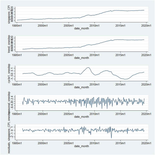
Table presents the summary statistic of “de-seasonalized” CPIs and their corresponding real exchange rate. Based on D’Agostino, Belanger test for normality behaviour, it seems that real exchange rates for most of the investigated countries exhibit non-normal distributions and demonstrate a positive skewness as well as kurtosis. Moreover, there are strong dependent structures (up to lag 40) which are shown by the auto correlogram and Ljung—Box test (Ljung & Box, Citation1978). The depreciation of the domestic currency against the dollars in investigated countries is observed. Based on the descriptive statistics shown in the first row of Table , on average, the SGP dollar gains 45 per cent its value against the US dollar. In contrary, other currencies seem to lose their value against the dollars during the period.
Table 1. Hurst’s exponents
Table 2. Descriptive statistics
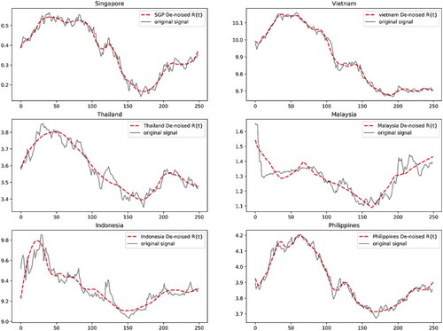
The real exchange rate patterns are plotted in Figure . The dashed lines in Firgure represent the smooth components which are deduced by using wavelet transform to “de-noising” the high-frequency oscillations.
Figure 2. Real exchange rate
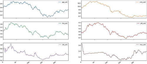
Figure 3. De-noised real exchange rate
It is appropriate to use a wide range of stationary tests for validating the effectiveness of the PPP in the long run. Table presents the test results for the real exchange rate . We use three tests (augmented Dickey–Fuller (ADF) (Citation1979), Phillips and Perron (Citation1988) and KPSS test (1992)) which are widely used in economics for attributing whether or not an economic time series is stationary. The Bayesian Information Criterion is utilized in order to decide an optimal lag for every real exchange rate pair. Three test results confirm strong denial on the assertion that all real exchange rate series are stationary process at 99 per cent. Following the results, all investigated real exchange rates series do not exhibit a clear pattern following the law of one price (PPP). Abuaf and Jorion (Citation1990), O’Connell (Citation1998) consider that the power of the stationary test is slightly below unity.
Table 3. Univariate stationary test results
We utilize the panel unit root test methods which were developed by Levin, Lin and Chu (LLC) (Citation2002), Breitung and Das (BT) (Citation2005), Harris and Tzavalis (HT) (Citation1999), Choi (Citation2001) (Fisher), Hadri (Hadri) (Citation2000), Im et al. (Citation2003) (IPS). These tests allow us to entangle the perplexity that the real exchange rate does exhibit stationary tendency in the long run, as presented in Table . The null hypothesis of the panel unit root test is the entire data set contains a unit root.
Table 4. Panel stationary test results
3.3. Insights of multi-resolution analysis
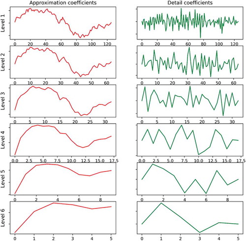
Figure visually explains how the multi-resolution analysis (MRA) aids in finding the long-run real exchange rate pattern in the most intuitive way. The SGP/USD real exchange rate is selected as the example for illustrating the multi-level analysis corresponding to different time horizon. It is worth considering that the MRA splits any given time series into two particular parts, to be named (i) detailed coefficients and (ii) averaging coefficients. The detailed coefficients account for the high-speed oscillations which result from arbitrage activities, whereas the averaging trends or long-term movements are reflected in the other half. In contrast, the detailed coefficients gradually approach averaging coefficients as a number of level increases. Another aspect of the MRA is the double of frequency resolution. After each level, the length of time series is cut into a half, which implies the double in our sampling frequency. We only present our application of MRA on the Singapore Dollar in Figure .
Figure 4. Multi-level decomposition of SGP/USD real exchange rate
4. Tests for the validity of the PPP and the prediction
4.1. PPP validation
The question now is that which specific time horizons that PPP takes its effect. In addressing the relationship between two parts of MRA’s output, Table incorporates our explanations which might be considered helpful for readers’ interpretation of the MRA mechanism. Table , in conjunction with Table , show the applications of the unit root test, which were previously conducted. The wavelet transformation, which is introduced in Section 3, provides a numerical embodiment of our time series under the terms of the “Detailed” coefficients and the “Averaging” coefficients. The “Detailed” coefficients explain the oscillations corresponding to the high frequencies in the frequency spectrum). The “Averaging” coefficients account for the coefficients corresponding to the low-speed oscillations or trend in the frequency spectrum). Additionally, we repeatedly apply the unit root test on each level of the MRA process, which comprises of detailed components and averaging components upon reaching maximum level obtained. The averaging coefficients which are hidden under many high-frequency fluctuations of six pairs of currency are stationary. These findings are possibly indifferent from dichotomy theory.
Table 5. Insights of the MRA mechanism
Table 6. Univariate stationary test results on six real exchange rate—Averaging coefficients
We report the univariate unit test results on detailed coefficients for each level of MRA in Table and unit root test results on averaging coefficients for each level in Table . The empirical test results strongly back up our set-forth assumption that the PPP tends to hold in the long run at 1 per cent level for three well-known types of univariate unit root test (KPSS, ADF and PP).
Table 7. Univariate stationary test results on six real exchange rate detailed coefficients
Real exchange rates for all currencies are reported to be stationary at 5 per cent after applying MRA 5 times successively (except for Vietnam with KPSS test, Thailand with both ADF and PP test, Malaysia with KPSS test). Moreover, the strong empirical evidence on the PPP validation is recorded at 1 per cent after six times of MRA successive application. In order to acquire the certainty on PPP validation, we decide to re-apply panel tests which mentioned in the previous section (LLC, HT, BT, IPS, Hadri, Fisher) on the average coefficients. The test’s results are reported in Table below.
Table 8. The multivariate test results on six averaging coefficients and detailed coefficients
The PPP validity seems independent of the variation in stationary tests. Following the consensus of results of the univariate stationary test, the confirmation on the validation of PPP remains in the LLC, IPS, HT, Hadri, Fisher test at 5 per cent confidence level. Overall, the mean-reverting pattern of the real exchange rate is consistent with the test results found in both Tables and . We conclude that at the time horizon approximately equal months, the real exchange rate takes 5.3 years for completing it cycle which is in agreement to the most precedented studied related to PPP (Rogoff, Citation1996; Vo and Vo, Citation2019b).
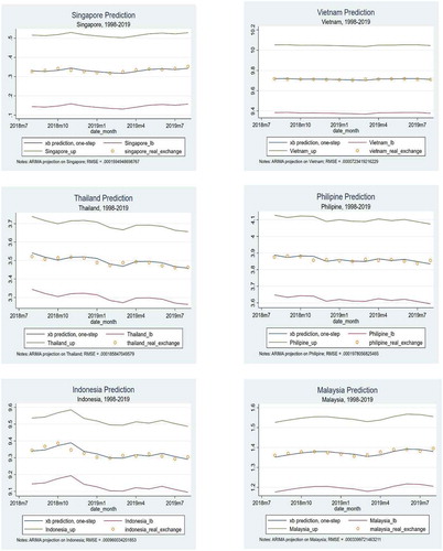
4.2. Prediction of the exchange rates
In this section, we use the averaging coefficients acquired from the MRA for prediction. Wavelet method not only filters out the high-pitch frequencies in accordance with arbitraging activities but also returns the pattern or the long-run movements of the real exchange rate. First, we reuse our original real exchange rate data which spans over 242 months (12/1998–08/2019) for comparative purpose. Next, the last 12 months (12 observations) are used as the baseline for our projection. ARIMA model is used to make a comparison to the baseline observations. The lags order used for ARIMA is determined by the Bayesian Information Criteria. The details of ARIMA given by the equation as follows:
where
corresponds to the parameters of the autoregressive part and moving average part of the ARIMA model. One step ahead
projection as
is computed. Root mean squared errors (RMSE) is considered as our measurements of effectiveness for projection which is calculated using the following equation:
Figure below presents the one-step projection. The method yields a significant accurate projection on real exchange rate movements by means of RMSE.
Figure 5. ARIMA on six real exchange rate series
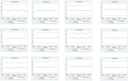
For the next step, we take S as the representation of the trend in real exchange rate series. The averaging coefficients S1 is de-noised and characterized by many turning points. The reason behinds this step is for the policy implication, which might attract many significant attentions. Visually, we call the S1 averaging series as the and measure the magnitude of variation in respect to time-lapse using the following equation:
Presumably, the coefficients is expected to be zero and
is expected to be −1. Hence, the robustness of our projection is also the robustness of slope and intercept of the above equation. Figure below demonstrates the test results for two coefficients
and
. The test results are all significant at the 5 per cent significance level, but the power of the estimated value remains relatively low. The results are shown in Figure .
Figure 6. The estimated alpha and beta coefficients
5. Conclusions and policy implications
This study is conducted to investigate the validity of the purchasing power parity (PPP) in the long-run using the multi-resolution analysis (MRA). The MRA has its root related to wavelet methodology, which has been widely utilized in signals processing, but the analysis is relatively new in applications in economic studies. Monthly data for the period from 1998 to 2019 for six key ASEAN countries are used in this study. Empirical findings from this paper indicate that the predicted real exchange rates exhibit good real-time properties because of the significant correlation between one-step ahead values and the wavelet measurements. Three significant insights corresponding to the interpretation of these dynamics can be summarized as follows. First, the mean-reverting pattern of the real exchange rate recurs itself for the period longer than five years. In this paper, the univariate and multivariate analyses are utilized to confirm this important finding. Second, the application of MRA provides many turning points of the real exchange rate, which could be utilized as a preference for an effective monetary system and an counter-cyclical fiscal policy. Moreover, the MRA method provides the central banks and the governments with a convincing pattern of real exchange rate movements in the future for policy purposes. Third, the validity of the real exchange rate forms a concrete basis for the efficiency of the currency markets in six ASEAN countries, meaning that the currency fair value is justified by the constant high-pitch activities.
Wavelet transformation is useful in physics and engineering. However, its applications and implications appear to be still unfamiliar to many economists. In addition to the capability of decomposition, the wavelet transformation also has the predictive ability which transforms the data into many turning points over the time domain. Counter-cyclical policies should be considered and initiated for stabilizing macroeconomic conditions when the values of the real exchange rates are off-track from their long-term patterns. Moreover, investors can consider the MRA method for predicting the price movement of their financial assets at different time horizons. On the ground of the findings obtained from this study, we recommend the use of the wavelet approach because of its credibility and applications in providing important insights into the financial markets for policymakers and practitioners.
Additional information
Funding
Notes on contributors
Duc Hong Vo
Duc Hong Vo is professor and practitioner of applied economics and finance. He has been working for the Australian public sector at the executive role since 2008. Duc is currently Head and Executive Director at the CBER – Research Center in Business, Economics and Resources at Ho Chi Minh City Open University, Vietnam. More than 80 papers from his research have been published in Journal of Economic Surveys; Renewable Energy; Applied Economics, North American Journal of Economics and Finance; Economics Letters; Journal of Intellectual Capital, Economic Papers; Journal of Asian Economics. His current research interests cover energy and environment; and applied financial economics.
Nhan Thien Nguyen
Nhan Thien Nguyen is completing the master degree at Vietnam-the Netherlands Programme in Vietnam. Nhan is a research associate at the CBER. His research interests include financial development and energy economics. He has published in Emerging Markets Finance and Trade; Cogent Business and Management and Borsa Istanbul Review.
References
- Abuaf, N., & Jorion, P. (1990). Purchasing power parity in the long run. The Journal of Finance, 45(1), 157–19. https://doi.org/10.1111/j.1540-6261.1990.tb05085.x
- Adler, M., & Lehmann, B. (1983). Deviations from purchasing power parity in the long run. The Journal of Finance, 38(5), 1471–1487. https://doi.org/10.1111/j.1540-6261.1983.tb03835.x
- Baqaee, D. (2010). Using wavelets to measure core inflation: The case of New Zealand. The North American Journal of Economics and Finance, 21(3), 241–255. https://doi.org/10.1016/j.najef.2010.03.003
- Breitung, J., & Das, S. (2005). Panel unit root tests under cross-sectional dependence. Statistica Neerlandica, 59(4), 414–433. https://doi.org/10.1111/j.1467-9574.2005.00299.x
- Choi, I. (2001). Unit root tests for panel data. Journal of International Money and Finance, 20(2), 249–272. https://doi.org/10.1016/S0261-5606(00)00048-6
- Clark, P. K. (1987). The cyclical component of U. S. economic activity. The Quarterly Journal of Economics, 102(4), 797–814. https://doi.org/10.2307/1884282
- Cotter, J., Dowd, K., & Loh, L. (2011). U.S. CORE INFLATION: A WAVELET ANALYSIS. Macroeconomic Dynamics, 15(4), 513–536. https://doi.org/10.1017/S1365100510000179
- Daubechies, I. (1992). Ten Lectures on Wavelets (1st ed.). Society for Industrial and Applied Mathematics.
- De Bondt, W. F. M., & Thaler, R. (1985). Does the stock market overreact? The Journal of Finance, 40(3), 793–805. https://doi.org/10.1111/j.1540-6261.1985.tb05004.x
- Dickey, D. A., & Fuller, W. A. (1979). Distribution of the estimators for autoregressive time series with a unit root. Journal of the American Statistical Association, 74(366), 427–431. doi:10.2307/2286348
- Dickey, D. A., & Fuller, W. A. (1979). Distribution of the estimators for autoregressive time series with a unit root. Journal of the American Statistical Association, 74(366), 427–31.
- Engel, C., & Rogers, J. H. (1996). How wide is the border?. American Economic Review, 86(5): 1112–1125.
- Granger, C. W. J., & Joyeux, R. (1980). An introduction to long-memory time series models and fractional differencing. Journal of Time Series Analysis, 1(1), 15–29. https://doi.org/10.1111/j.1467-9892.1980.tb00297.x
- Haar, A. (1910). Zur theorie der orthogonalen funktionensysteme: Erste mitteilung. Mathematische Annalen, 69(3), 331–371. https://doi.org/10.1007/BF01456326
- Hadri, K. (2000). Testing for stationarity in heterogeneous panel data. The Econometrics Journal, 3(2), 148–161. https://doi.org/10.1111/1368-423X.00043
- Harris, R. D., & Tzavalis, E. (1999). Inference for unit roots in dynamic panels where the time dimension is fixed. Journal of Econometrics, 91(2), 201–226. https://doi.org/10.1016/S0304-4076(98)00076-1
- Harvey, A. C. (1985). Trends and cycles in macroeconomic time series. Journal of Business and Economic Statistics, 3(3), 216–227. doi:10.2307/1391592
- Heisenberg, W. (1971). Physics and beyond: Encounters and conversations.
- Hosking, J. R. M. (1981). Fractional differencing. Biometrika, 68(1), 165–176. https://doi.org/10.1093/biomet/68.1.165
- Hurst, H. (1951). Long term storage capacity of reservoirs. Transaction of the American Society of Civil Engineers, 116(1), 770–799. https://cedb.asce.org/CEDBsearch/record.jsp?dockey=0292165.
- Im, K. S., Pesaran, M. H., & Shin, Y. (2003). Testing for unit roots in heterogeneous panels. Journal of Econometrics, 115(1), 53–74. https://doi.org/10.1016/S0304-4076(03)00092-7
- Knetter, M. M. (1994). Why are retail prices in Japan so high? Evidence from German export prices. International Journal of Industrial Organization, 15(5), 549–572. https://doi.org/10.1016/S0167-7187(96)01021-1
- Kwiatkowski, D., Phillips, P., Schmidt, P., & Shin, Y. (1992). Testing the null hypothesis of stationarity against the alternative of a unit root: How sure are we that economic time series have a unit root? Journal of Econometrics, 54(1–3), 159–178. https://doi.org/10.1016/0304-4076(92)90104-Y
- Levin, A., Lin, C. F., & Chu, C. S. J. (2002). Unit root tests in panel data: Asymptotic and finite-sample properties. Journal of Econometrics, 108(1), 1–24. https://doi.org/10.1016/S0304-4076(01)00098-7
- Ljung, G. M., & Box, G. E. (1978). On a measure of lack of fit in time series models. Biometrika, 65(2), 297–303. https://doi.org/10.1093/biomet/65.2.297
- Malkiel, B. G. (2003). The efficient market hypothesis and its critics. Journal of Economic Perspectives, 17(1), 59–82. https://doi.org/10.1257/089533003321164958
- Mallat, S., & Zhong, S. (1992). Characterization of signals from multiscale edges. IEEE Transactions on Pattern Analysis and Machine Intelligence, 14(7), 710–732. https://doi.org/10.1109/34.142909
- Nielsen, B. (2001). Order determination in general vector auto regressions. Working paper, Department of Economics, University of Oxford and Nuffi eld College.
- O’Connell, P. G. (1998). The overvaluation of purchasing power parity. Journal of International Economics, 44(1), 1–19. https://doi.org/10.1016/S0022-1996(97)00017-2
- Patinkin, D. (1965). Money, interest, and prices; an integration of monetary and value theory (No. 04; HG221, P3 1965.).
- Paulsen, J. (1984). Order determination of multivariate autoregressive time series with unit roots. Journal of Time Series Analysis, 5(2), 115–127. https://doi.org/10.1111/j.1467-9892.1984.tb00381.x
- Percival, D. B., & Walden, A. T. (2000). Wavelet methods for time series analysis. Cambridge University Press.
- Phillips, P. C. B., & Perron, P. (1988). Testing for a unit root in time series regression. Biometrika, 75(2), 335–346. https://doi.org/10.1093/biomet/75.2.335
- Qian, B., & Rasheed, K. (2004). Hurst exponent and financial market predictability [Paper presentation]. IASTED conference on Financial Engineering and Applications (FEA 2004)
- Rogoff, K. (1996). The purchasing power parity puzzle. Journal of Economic Literature, 34(2), 647–668. https://www.jstor.org/stable/2729217?seq=1
- Roll, R. (1979). Violations of purchasing power parity and their implications for efficient international commodity markets. In M. Sarnat & G. Szego (Eds.), International Finance and Trade (pp. 133 -176). Cambridge: Ballinger.
- Salehizadeh, M., & Taylor, R. (1999). A test of purchasing power parity for emerging economies. Journal of International Financial Markets, Institutions and Money, 9(2), 183–193. https://doi.org/10.1016/S1042-4431(99)00006-2
- Schleicher, C. (2002). An introduction to wavelets for economists. Bank of Canada.
- Tiwari, K. A., Dar, B. A., & Bhanja, N. (2013). Oil price and exchange rates: A wavelet based analysis for India. Economic Modelling, 31(C), 414–422.
- Tsay, R. S. (1984). Order Selection in Nonstationary Autoregressive Models. Annals of Statistics, 12(4), 1425–1433. https://doi.org/10.1214/aos/1176346801
- Vo, H. L., & Vo, H. D. (2019a). Application of wavelet-based maximum likelihood estimator in measuring market risk for fossil fuel. Sustainability, 11(10), 2843. https://doi.org/10.3390/su11102843
- Vo, H. L., & Vo, H. D. (2019b). Long-run dynamics of exchange rates: A multi-frequency investigation. The North American Journal of Economics and Finance. https://doi.org/10.1016/j.najef.2019.101125