Extreme return-volume relationship in cryptocurrencies: Tail dependence analysis

Abstract

We explore extreme return-volumes dependence among different cryptocurrencies such as Bitcoin, Ethereum, Ripple, and Litecoin by using the Copula approach. We use Student-t, Frank, Clayton, Survival Clayton, Gumbel, and SJC copulas. We filter out margins by using the EGARCH model for return series and GARCH model for volume series. Evidence of significant symmetric dependence between return-volume is not found due to insignificance of student-t and Frank copula parameters. In a return-volume relationship, coefficients of lower tail dependence are significant for Bitcoin, Ripple, and Litecoin which means that low returns are followed by low volumes. Lower tail dependence for the return-volume relationship is stronger than the upper tail dependence for Bitcoin, Ripple, and Litecoin. Moreover, for negative return-volume, left tail dependence coefficients are significant for Ripple and Litecoin, which means that high returns are followed by low volumes for Ripple and Litecoin. Our investigation shows that investors (buyer or seller) are very careful in extreme market conditions for both Ripple and Litecoin. Extreme upper tail and lower tail dependence coefficients are insignificant for Ethereum.

Keywords:

• cryptocurrencies
• EGARCH-copula model
• return-volume
• upper tail dependence
• negative returns

PUBLIC INTEREST STATEMENT

• This paper investigates extremely high or low returns on trading volumes for leading cryptocurrencies.

• Extreme return-volumes dependence among different cryptocurrencies by employing Copula methodology.

• Investigation shows that investors (buyer or seller) are very careful in extreme market conditions for both Ripple and Litecoin.

• Finding is unique to the cryptocurrency market, which might be due to the highly volatile nature of cryptocurrencies.

• Findings of this paper are very informative for crypto-traders as they provide insightful information about the dependence between cryptocurrency positive and negative return-volume, especially in the extreme market conditions of cryptocurrencies.

• Crypto-traders can now have a better understanding of the return-volume dependence of high volatility cryptocurrencies.

1. Introduction

One of the most significant innovations in finance has been the creation and development of cryptocurrencies. These digital means of exchange have been the focus of extensive news coverage, especially the bitcoin, with a primary focus on the tremendous potential return and the high level of risk. This paper aims to study the extreme negative and positive return-volume relationship in the four most representative cryptocurrencies: Bitcoin, Ethereum, Litecoin, and Ripple. Because understanding the return–volume nexus can provide many useful signals for market participants to determine investment strategies or to rebalance their portfolios, a great number of theoretical and empirical studies have attempted to explain and explore this nexus from several different directions.

The return-volume relationship has been analyzed from many different points of view in the literature (e.g., Clark, 1973; Crouch, 1970; Granger & Morgenstern, 1963; Rogalski, 1978; Tauchen & Pitts, 1983; Westerfield, 1977). As investors revise their reservation prices based on the arrival of new information to the market, trading volume had been used to measure disagreement among market participants by using mixture models in Epps and Epps (1976). The level of trading volume increases as the degree of disagreement among traders’ spreads. Their model exhibits a positive causal relation running from trading volume to absolute stock returns. Jain and Joh (1988) found a strong contemporaneous relation between trading volume and returns by using hourly common stock trading volume and return on NYSE. Further, they have also found the lead-lag relationship between trading volume and returns lagged up to 4 hours. Moreover, trading volume-returns relation is higher for positive returns than for negative returns.

Chen et al. (2001) studied the dynamic relation between trading volume, returns, and volatility of stock indices of nine national markets. They found a positive dependence between trading volume and absolute returns. They have also shown that trading volume provides some information about the returns process. Gunduz and Hatemi-J (2005) explored the causal relationship between stock prices and volume of Hungary, the Czech Republic, Russia, Poland, and Turkey stock markets. Floros and Vougas (2007) had examined the relationship between trading volume and returns in the Greek Stock Index Futures Market and found a significant positive contemporaneous relationship between trading volume and returns in the case of FTSE/ASE-20. Further, the results for FTSE/ASE Mid 40 do not provide any evidence of the relationship between trading volume and returns. Furthermore, the literature on return-volume dependence can be found in the papers of Attari et al. (2012) and Naeem et al. (2014).

There is a vivid debate in the literature about the correlation between volatility and return volume. It is nowadays accepted that they tend to show relatively strong upper tail dependence (see, e.g.,, Rossi et al., 2013). Ning and Wirjanto (2009) found upper tail dependence in return and volume series of East Asian stock markets. However, Chen et al. (2001) explain that negative return in period t raises volatility in period t +1. Further, an explanation can be seen from Bae et al. (2007), that when volatility increases, risk increases and returns decrease. If we combine the work of Rossi et al. (2013) and the fact mentioned in the paper by Chen et al. (2001) and Wagner (2012), then one should expect positive dependence between low returns and volumes.

The extensive literature on the economics and finance aspects of cryptocurrencies have recently intensified. For instance, Akbulaev and Salihova (2020) examined the relationship between cryptocurrencies prices and volume using the VAR modeling approach and found the transaction volume change is negatively affected by the past thirteen-day values and the price change is affected by 1% of the significance level.

Zhang et al. (2018) explored the Return-Volume Relationship for Bitcoin Market. They found anti-persistent behavior for the return-volume in the Bitcoin markets. Balcilar et al. (2017) employ a non-parametric causality-inquantiles test to analyze the causal relationship between trading volume and Bitcoin returns and volatility. Their results reveal that volume can predict returns—except in Bitcoin bear and bull market regimes. They suggested that this result highlights the importance of modeling nonlinearity and accounting for the tail behavior when analyzing causal relationships between Bitcoin returns and trading volume.

However, there are few studies explain extreme return-volume dependence in the major cryptocurrencies that have been gaining ground and attracted the attention of individual and institutional investors (Corbet et al., 2019; Hashemi Joo et al., 2020). Interestingly, many cryptocurrencies offer outstanding price growth in relatively short periods, exceeding a hundred percent levels (Kristoufek, 2013), but with extreme volatility (Chu et al., 2017; Katsiampa et al., 2018; Koutmos, 2018; Takaishi, 2020; Urquhart, 2017). Cryptocurrencies are categorized by large price fluctuations, and these price movements are often associated with surges in transaction volumes, suggesting a dependence between transaction volume and price (Balcilar et al., 2017).

Moreover, Koo et al. (2020) investigate the tail behavior of four major Cryptocurrencies by using the Autoregressive Frechet model for conditional maxima. Using five-minute-high frequency data, they report time-evolving tails as well as provide a straightforward measure of tails asymmetry for positive and negative intra-day returns. Tiwari et al. (2020) examine the dependence and contagion risk between Bitcoin (BTC), Litecoin (LTC), and Ripple (XRP) using non-parametric mixture copulas. Their results provide evidence of significant risk contagion among price returns of major cryptocurrencies, both in bull and bear markets. Garcia-Jorcano and Muela (2020) study the properties of Bitcoin as a diversifier asset and hedge asset against the movement of international market stock indices by employing copula methodology. They found that under normal market conditions, Bitcoin might act as a hedge asset against the stock price movements, however, under extreme market conditions, the role of Bitcoin might change from hedge to diversifier. In a time-varying copula analysis, they found that the role of Bitcoin as a hedge asset might fail on a high number of days. Naeem et al. (2020) analyze the average and extreme dependence between returns and trading volumes of three main cryptocurrencies (Bitcoin, Ethereum, and Litecoin) by time-varying copula methodology. They found asymmetric tail behavior and show that extreme returns are associated with extreme trading volumes, and tail dependence is stronger when returns and volumes are high than when returns and volume are low. Maghyereh and Abdoh (2020) they study the tail dependence between returns for Bitcoin and other financial assets using the novel “quantile cross-spectral dependence” approach. Their findings support the notion that Bitcoin can provide financial diversification due to the presence of right tail dependence between Bitcoin and other Markets. Poyser (2019) explores the association between Bitcoin’s market price and a set of internal and external factors by employing the Bayesian structural time series approach (BSTS). Their results show that Bitcoin’s price is negatively associated with the price of gold as well as the exchange rate between Yuan and US Dollar, while positively correlated to the stock market index, USD to Euro exchange rate, and diverse signs among the different countries’ search trends. Xu et al. (2020) analyze the tail-risk interdependence among 23 cryptocurrencies and identifies the systemically important cryptocurrencies using the TENET. They found significant risk spillover effect exists and the degree of the total connectedness of all the sampled cryptocurrencies increases steadily over time. Further, Bitcoin is the largest systemic risk receiver while Ethereum is the largest systemic risk emitter. The literature mainly discusses cryptocurrencies dependence with each other or with other markets. Literature for return-volume dependence is limited for cryptocurrencies. Further, we have not found any evidence of negative return-volume dependence in cryptocurrencies.

This paper aims to investigate extreme negative and positive return–volume dependence in four major cryptocurrencies, Bitcoin, Ethereum, Ripple, and Litecoin, using copula methodology. Firstly, we select the usual GARCH model based on the log-likelihood to filter out margins. Secondly, we check both negative and positive return-volume dependence by employing Clayton, Gumbel, and symmetrized Joe Clayton (SJC) copulas. This represents an extension to previous studies such as Bouri et al. (2019), Naeem et al. (2014), and Bouri et al. (2019) limit their analyses to the use of static copulas to make inferences about the presence of Granger-causality within a quantile-based approach. While Naeem et al. (2014) use dynamic copula methodology to exploit extreme dependence between return and volume but they did not consider extreme dependence in the negative return-volume relationship.

If cryptocurrencies returns are well described by the multivariate normal distribution, then the linear correlation is an appropriate dependence measure. However, in our case, a simple exploratory and graphical analysis of both returns and volumes distributions suggest fat tails, heteroscedasticity, clustering, and other non-Gaussian features. Thus, the linear correlation might be deceptive in our analysis. Alternative measures of dependence based on copula methods combined with the EGARCH model are considered here. The copula approach is widely used in quantitative finance literature. Here we combine copula modeling with a univariate EGARCH model for returns of cryptocurrencies to properly calibrate a joint model for returns and volumes.

Our results show strong evidence of extreme dependence, but find lower tail dependence to be much stronger than upper tail dependence. Such evidence of asymmetric behavior at extreme levels of dependence in all four cryptocurrencies does not conform to the related evidence from equity markets, which highlights some differences in return-volume between cryptocurrency and stock markets. The remainder of this paper is organized as follows: section two introduces the EGARCH model. Section three describes the copula methodology. Section four reports empirical results and section five concludes with implications, limitations, and future work recommendations.

2. EGARCH model

2.1. ARCH model

ARCH models based on the variance of the error term at time t depends on the realized values of the squared error terms in previous time-periods. The model is specified as:

(2.1) $y_t=u_t$(2.1)

$u_t\text{~}N\left(0,h_t\right)$

(2.2) $h_t={\alpha }_0+\sum _{t=1}^q{\alpha }_j{u}_{t-i}^2$(2.2)

This model is referred to as ARCH(q), where q refers to the order of the lagged squared returns included in the model. If we use the ARCH (1) model it becomes

(2.3) $h_t={\alpha }_0+{\alpha }_1{u}_{t-1}^2$(2.3)

Since $h_t$is a conditional variance, its value must always be strictly positive; a negative variance at any point in time would be meaningless. To have positive conditional variance estimates, all of the coefficients in the conditional variance are usually required to be non-negative. Thus, coefficients must be satisfying α₀ >0and α₁ >0.

2.2. GARCH model

Bollerslev (1986) developed the GARCH (p, q) model. The model allows the conditional variance of the variable to be dependent upon previous lags; first lag of the squared residual from the mean equation and present news about the volatility from the previous period which is as follows:

(2.4) $h_t={\alpha }_0+\sum _{i=1}^q{\alpha }_i{u}_{t-i}^2+\sum _{i=1}^p{\beta }_i{h}_{t-i}$(2.4)

In the literature most used and simple model is the GARCH (1,1) process, for which the conditional variance can be written as follows:

(2.5) $h_t={\alpha }_0+{\alpha }_1{u}_{t-1}^2+{\beta }_1{h}_{t-1}$(2.5)

Under the hypothesis of covariance stationarity, the unconditional variance $h_t$can be found by taking the unconditional expectation of equation 5.

We find that

(2.6) $h={\alpha }_0+{\alpha }_{1}h+{\beta }_{1}h$(2.6)

Solving the equation (2.5)(2.5) $h_t={\alpha }_0+{\alpha }_1{u}_{t-1}^2+{\beta }_1{h}_{t-1}$(2.5) , we have

(2.7) $h=\frac{{\alpha }_0}{1-{\alpha }_1-{\beta }_1}$(2.7)

For this unconditional variance to exist, it must be the case that${\alpha }_1+{\beta }_1<1$ and for it to be positive, we require that${\alpha }_0>0$.

2.3. Exponential GARCH

Exponential GARCH (EGARCH) was proposed by Nelson (2006) which has a form of leverage effects in its equation. In the EGARCH model the specification for the conditional covariance is given by the following form:

(2.9) $log\left(h_t\right)={\alpha }_0+\sum _{j=1}^q{\beta }_{j}log\left(h_{t-j}^{\hspace{0.17em}}\right)+\sum _{i=1}^p{\alpha }_i\left|\frac{u_{t=i}}{\sqrt{h_{t=i}}}\right|+\sum _{k=1}^r{\gamma }_k\frac{u_{t-k}}{\sqrt{h_{t-k}}}$(2.9)

Two advantages stated in Brooks (2008) for the pure GARCH specification; by using $log\left(h_t\right)$even if the parameters are negative, will be positive and asymmetries are allowed for under the EGARCH formulation.

The equation ${\gamma }_k$represents leverage effects which account for the asymmetry of the model. While the basic GARCH model requires the restrictions the EGARCH model allows unrestricted estimation of the variance.

If ${\gamma }_k<0$it indicates leverage effect exists and if ${\gamma }_k\ne 0$impact is asymmetric. The meaning of leverage effect bad news increase volatility.

Applying the process of GARCH models to return series, it is often found that GARCH residuals still tend to be heavy-tailed. To accommodate this, rather than to use normal distribution the Student’s t and GED distribution used to employ ARCH/GARCH type models.

2.4. Statistical inference

Parameter estimation of GARCH and EGARCH model is commonly carried out by using the maximum likelihood method with the normality assumption for ε_t. However, as mentioned by Kang et al. (2010) and Tang and Shieh (2006), the residuals estimated from the GARCH type model frequently exhibits lepto-kurtosis and asymmetry. To overcome these problems the Student-t distribution has been considered for the innovations process. Given the random variable ε_t~t_v(0,1,v) the log-likelihood function is defined as follows:

(2.10) $\begin{array}{rl}& log\left(L;\mathrm{\Theta }\right)=T\left\{\mathrm{l}\mathrm{o}\mathrm{g}\mathrm{\Gamma }\left(\frac{\nu +1}{2}\right)-log\mathrm{\Gamma }\left(\nu /2\right)-\frac{1}{2}log\left[\pi \left(\nu -2\right)\right]\right\}\\ & -\sum _{t=1}^T\left[log{{\sigma }^2}_t+\left(1+\nu \right)log\left(1+\frac{{{\epsilon }^2}_t}{{{\sigma }^2}_t\left(\nu -2\right)}\right)\right]\end{array}$(2.10)

Matlab garchfit function has been used to estimate the parameters of the GARCH and EGARCH models. then the standardized residuals are calculated as follows.

(2.11) ${\epsilon }_t=r_t/\sqrt{{\sigma }_t}$(2.11)

3. The copula methodology

Copula-based models provide a great deal of flexibility in modeling multivariate distributions. This allows the researcher to specify the models for the marginal distributions separately from the dependence structure (copula) that links them to form a joint distribution. From an inferential perspective, the copula representation facilitates the estimation of the model in stages, reducing the computational burden.

Several surveys of copula theory and applications have appeared in the literature to date: Nelson (2006) and Joe (1997) are the most important textbooks on copula theory, providing detailed introductions to copulas and dependence modeling, with an emphasis on statistical foundations. Kurowicka and Joe (2011) represent an up-to-date survey on copula and vine-copula applications Cherubini et al. (2004) present an introduction to copulas using methods from mathematical finance, MecNeil et al. (2005) present an overview of copula methods for risk management. Patton (2009) presents a summary of applications of copulas to financial time series. Jondeau and Rockinger (2006) proposed a GARCH-Copula approach to measure the dependence structure of stock markets. It is well known that the analysis of dependence analysis, especially of extreme events, plays a crucial role in financial applications such as portfolio selection, Value-at-Risk, and international asset allocation.

A copula model is a way of constructing the joint distribution of a random vector$X=\left(X_1,\cdots ,X_m\right)$. It is possible to show that there always exists an m-variate function C: [0, 1] ^m → [0, 1], such that

(3.1) $\left(x_1,\cdots ,x_m\right)=C\left(F_1\left(x_1\right),\cdots ,F_m\left(x_m\right)\right)$(3.1)

The copula function C is a cumulative distribution function (CDF) with uniform margins on [0, 1]: it binds together the univariate cumulative distribution functions F₁, F₂, and F_m to produce the m-variate CDF F. The three main properties are

1. $C(x_1,x_2,\cdots x_m)$is increasing in component $x_i$

$ii.)C\left(1,\cdots ,1,x_i,1,\cdots ,1\right)=x_{i}foralli=1,\cdots ,m,x_i\in \left[0,1\right]$

1. For all $\left(a_1,\cdots ,a_m\right),\left(b_1,\cdots ,bm\right)\in {\left[0,1\right]}^{m}with{a}_i\le b_i$ one has

$\sum _{i_1=1}^2\cdots \sum _{i_m}^2{\left(-1\right)}^{i_1+\cdots +{\mathcal{B}}_m}C\left(x_{1i_1},\cdots ,x_{m{i}_m}\right)\ge 0$

where $x_{j1}=a_{j}and{x}_{j2}=b_j\mathrm{\forall }j\in \left\{1,\cdots ,m\right\}$

For any continuous multivariate distribution, the copula representation is unique. If the marginal $F_1,\cdots ,F_m$ is not all continuous it can be shown that the joint CDF still has a copula representation although this representation is not unique. In the continuous case, one can take derivatives of both side of Equation (3.1)(3.1) $\left(x_1,\cdots ,x_m\right)=C\left(F_1\left(x_1\right),\cdots ,F_m\left(x_m\right)\right)$(3.1) , we get the density representation of F:

(3.2) $\begin{array}{rl}& f\left(x_1,x_2,\cdots ,x_m\right)=\frac{{\mathrm{\partial }}^{m}F\left(x_1,\cdots ,x_m\right)}{\mathrm{\partial }{x}_1,\cdots ,\mathrm{\partial }{x}_m}=\frac{{\mathrm{\partial }}^{m}C\left(F_1\left(x_1\right),\cdots ,F_m\left(x_m\right)\right)}{\mathrm{\partial }{F}_1\left(x_1\right)\cdots \mathrm{\partial }{F}_m\left(x_m\right)}\times f_1\left(x_1\right)\times \cdots \times f_m\left(x_m\right)\\ & =c\left(F_1\left(x_1\right),\cdots ,F_m\left(x_m\right)\right)\times \prod _{i=1}^m{f}_i\left(x_i\right)\end{array}$(3.2)

where $c\left(u_1,\cdots ,u_m\right)$ is the density of copula C, and $f_i\left(x_i\right)$ is the density of i-th margin. The joint use of GARCH and Copula models separates the temporal dependence, absorbed by the univariate GARCH structure, and the co-dependence among different variables, which is captured by the copula model.

3.1. Tail dependence and some bivariate copulas

In this paper, we use the copula approach to measure the tail dependence between the return and volume among four cryptocurrencies, so we keep focus on the two-dimensional case only. We can use the tail dependence coefficient to measure the concordance between the extreme events of different random variables. It is expressed in terms of a conditional probability that the asset X will incur a large loss (or gain), given that the asset Y also experiences a large loss (or gain). We consider two random variables X and Y, with joint continuous CDF F, copula C, and margins F_X; F_Y; the lower tail dependence and the upper tail dependence are defined as follows:

(3.3) ${\lambda }_L=\underset{u\to 0^{+}}{lim}Pr\left(F_X\left(x\right)<u\right)|F_Y\left(y\right)<u)=\underset{u\to 0^{+}}{lim}\frac{C\left(u,u\right)}{u}$(3.3)

(3.4) ${\lambda }_U=\underset{u\to 1^{-}}{lim}Pr\left(F_X\left(x\right)>u\right)|F_Y\left(y\right)>u)=\underset{u\to 1^{-}}{lim}\frac{1-2u+C\left(u,u\right)}{1-u}$(3.4)

Intuitively, if ${\lambda }_L$ and ${\lambda }_U$exist and fall in (0, 1], X and Y show lower or upper tail dependence. On the other hand, if ${\lambda }_L$and ${\lambda }_U$ are equal to 0, one can say that the two variables are independent in the tails, so extreme events seem to occur independently. We can describe different tail dependence behavior by choosing the appropriate copula model

3.1.1. Gaussian copula and student t-copula

These are symmetric and elliptical copulas. In the bivariate case the Gaussian copula is defined by the following expression:

(3.5) $\begin{array}{rl}& C_{\rho }^G\left(u,v\right)={\mathrm{\Phi }}_{\rho }\left({\mathrm{\Phi }}^{-1}\left(u\right),{\mathrm{\Phi }}^{-1}\left(v\right)\right)\\ & \underset{-\mathrm{\infty }}{\overset{{\mathrm{\Phi }}^{-1}\left(u\right)}{\int }}\underset{-\mathrm{\infty }}{\overset{{\mathrm{\Phi }}^{-1}\left(v\right)}{\int }}\frac{1}{2\pi \sqrt{1-{\rho }^2}}exp\left\{-\frac{s^2-2\rho st+t^2}{2\left(1-{\rho }^2\right)}\right\}dsdt\end{array}$(3.5)

where ${\mathrm{\Phi }}_{\rho }$the bivariate normal cumulative distribution function with linear correlation coefficient is $\rho \in \left[0,1\right],\mathrm{\Phi }$ is the standard normal cumulative distribution function and ${\mathrm{\Phi }}^{-1}$ is its inverse function. We can see that the bivariate Gaussian copula density is symmetrical, so it has a weak capability to capture asymmetrical dependence. It implies that if we go far into the tail, the extreme events tend to be independent, even though we choose a very high correlation. The t-copula is corresponding to a Student t distribution. It is defined by:

(3.6) $\begin{array}{rl}& C_{\nu ,\rho }^t=t_{\nu ,\rho }\left(t_{\nu }^{-1}\left(u\right),t_{\nu }^{-1}\left(v\right)\right)\\ & =\frac{\mathrm{\Gamma }\left(\frac{\nu }{2}+1\right)}{\mathrm{\Gamma }\left(\frac{\nu }{2}\right)\pi \sqrt{1-{\rho }^2}}\underset{-\mathrm{\infty }}{\overset{t_{\nu }^{-1}\left(u\right)}{\int }}\underset{-\mathrm{\infty }}{\overset{t_{\nu }^{-1}\left(v\right)}{\int }}1+\frac{-\left(s^2+2\rho st+t^2\right)}{2\left(1-{\rho }^2\right)}dsdt\end{array}$(3.6)

where $t_{\nu ,\rho }$ is the CDF of a two-dimensional t distribution with $\nu$ degree of freedom and correlation $\rho$. The t-copula also has symmetric shape, upper and lower tail dependence is identical, and it is determined by $\nu$ and$\rho$ When $\nu$ gets large, then t-copula decays to a Gaussian copula. The expression of ${\lambda }_L$ and ${\lambda }_U$ follows:

(3.7) ${\lambda }_L={\lambda }_U=2T_{\nu +1}\left(\frac{\sqrt{\left(\nu +1\right)\left(1-\rho \right)}}{\sqrt{\rho +1}}\right)$(3.7)

where $T_{\nu +1}$ is the CDF of the scalar Student t distribution with $\nu +1$ degrees of freedom (Demarta & McNeil, 2005).

3.1.2. Archimedean copulas

Archimedean copulas are defined through their generator functions. Generally, if a function $\phi :\left[0,1\right]\to \left[0,\mathrm{\infty }\right]$with the continuous derivative is decreasing and convex, it can be considered as a generator function of the Archimedean copula. By definition an-dimensional Archimedean copula has the following expression: $C\left(u_1,u_2,\cdots ,u_n\right)={\phi }^{-1}\left(\phi \left(u_1\right)+\phi \left(u_2\right)+\cdots +\phi \left(u_n\right)\right),$ different generator function creates different Archimedean copula. More details about the generator function can be found in Joe (1997) and Nelson (2006). In our case, the copula function is defined by:

(3.8) $C\left(u,v\right)={\phi }^{-1}\left(\phi \left(u\right)+\phi \left(v\right)\right)if\phi \left(u\right)+\phi \left(v\right)\le \phi \left(0\right)$(3.8)

where $\phi \left(u\right)$ is a $C^2$ function with $\phi \left(1\right)=0,{\phi }^{\prime }⟨0,{\phi }^{\prime \prime }⟩0$.

Examples of Archimedean copulas include the following

3.1.3. Clayton copula

The Clayton copula has the following form:

(3.9) $C\left(u,v;\rho \right)=max{\left[\left(u^{-\rho }-v^{-\rho }-1,0\right)\right]}^{-1/\rho }\rho \in \left(-1,+\mathrm{\infty }\right)\setminus \left\{0\right\}$(3.9)

Where is the dependence parameter${\lambda }_L=2^{-1/\rho },{\lambda }_U=0.$When$\rho \to 0$, the margins tend to be independent, oppositely when$\rho \to \mathrm{\infty }$, the margins tend to be strongly dependent. Clayton copula is asymmetric and it shows stronger low tail dependence. It can be proved that the components of a Gaussian copula are asymptotically independent.

3.1.4. Frank copula

The Frank copula is defined by:

(3.10) $\begin{array}{rl}& C\left(u,v;\rho \right)=-\frac{1}{\rho }log\left\{\frac{(e^{-\rho u}-1)\left(e^{-\rho v}-1\right)}{e^{-\rho }-1}-1\right\}\\ & \rho \in \left(-\mathrm{\infty },0\right){\cup }^{\left(0,+\mathrm{\infty }\right)}\end{array}$(3.10)

Just like Gaussian copula, Frank copula is symmetric in both tails and it is not sensitive to the relationship between the extreme negative values or between the extreme positive values. There is strong dependence in the center of the distribution. This means that Frank copula fails to capture tail dependence behavior and it suggests that it is suited to use when the tail dependence is relatively weak.

3.1.5. Gumbel copula

The Gumbel copula is an asymmetric extreme value copula, which takes the following expression:

(3.11) $C\left(u,v;\rho \right)=exp{\left[{(-lnu)}^{\rho }+\left(-ln{v}^{-\rho }\right)\right]}^{-1/\rho }\rho \in \left[1,\mathrm{\infty }\right]$(3.11)

where $\rho$ is a dependence parameter that describes different dependence behavior, ${\lambda }_L=0,{\lambda }_U=2-2^{1/\rho }.$When $\rho \to \mathrm{\infty }$ the margins show totally dependence, while $\rho$ = 1 corresponds to independence case. Unlike the Clayton copula, Gumbel copula deals with upper tail dependence. If two margins perform simultaneous extreme upper tail values, the Gumbel copula should be an appropriate considerable choice.

3.1.6. The symmetrized Joe–Clayton copula

Joe (1997) constructs the copula by taking a particular Laplace transformation of Clayton’s copula. The Joe–Clayton copula is:

(3.12) $C_{JC}\left(u,v|{\tau }^U,{\tau }^L\right)=1-{\left(1-{\left\{{\left[1-{\left(1-u\right)}^k\right]}^{-\gamma }+{\left[1-{\left(1-v\right)}^k\right]}^{-\gamma }-1\right\}}^{-1/\gamma }\right)}^{1/k}$(3.12)

where$k=\frac{1}{{log}_2(2-{\tau }^U)}$, $\gamma =\frac{-1}{{log}_2({\tau }^L)}$ and ${\tau }^i\in \left(0,1\right)$

are the measures of the upper- and lower-tail dependencies, respectively. Patton’s (2006) modified Joe–Clayton (JC) copula for which the density is as follows.

(3.13) $C_{SJC}\left(u,v|{\tau }^U,{\tau }^L\right)=\frac{1}{2}\left(C_{JC}\left(u,v|{\tau }^U,{\tau }^L\right)+C_{JC}\left(1-u,1-v|{\tau }^U,{\tau }^L\right)+u+v-1\right)$(3.13)

The SJC copula is symmetric when ${\tau }^U={\tau }^L$ and asymmetric otherwise.

3.2. Copula parameters estimation

Most of the methods for copula parameter estimation are related to Maximum Likelihood procedures. The standard ML method which estimates both marginal parameters and copula parameters simultaneously is also named the one-step method. Mashal and Naldi (2002) noted that this method is computationally costly, and when the data sets are not sufficiently large, the ML estimators seem to be ineffective. The inference function for the margins method (IMF) is based on the work of Joe and Xu (1996). The estimation procedure is split into two steps; the first one estimates the parameters of the marginal distributions. In the second step one tries to estimates the copula parameters, conditionally on the values of estimates obtained at the first step. This approach offers computational convenience, although it may be sensitive to the choice of marginal distributions form. A poor estimator of the copula parameter might be a consequence of an inappropriate marginal distribution. There is also an alternative, two steps method, named Canonical Maximum Likelihood (CML). Unlike IMF method, in the ’CML’ approach the transformation is done by using empirical CDF function to obtain uniform margins, which are used in copula parameter estimation.

Given two-time series ${\left\{X\right\}}_{t=1}^T$and${\left\{Y\right\}}_{t=1}^T$, let Ω be the parameter space, $a_x\in \mathrm{\Omega },a_y\in \mathrm{\Omega }$denote marginal parameters for X and Y, while $\theta \in \mathrm{\Omega }$denotes copula parameters. From Equation 3.2(3.2) $\begin{array}{rl}& f\left(x_1,x_2,\cdots ,x_m\right)=\frac{{\mathrm{\partial }}^{m}F\left(x_1,\cdots ,x_m\right)}{\mathrm{\partial }{x}_1,\cdots ,\mathrm{\partial }{x}_m}=\frac{{\mathrm{\partial }}^{m}C\left(F_1\left(x_1\right),\cdots ,F_m\left(x_m\right)\right)}{\mathrm{\partial }{F}_1\left(x_1\right)\cdots \mathrm{\partial }{F}_m\left(x_m\right)}\times f_1\left(x_1\right)\times \cdots \times f_m\left(x_m\right)\\ & =c\left(F_1\left(x_1\right),\cdots ,F_m\left(x_m\right)\right)\times \prod _{i=1}^m{f}_i\left(x_i\right)\end{array}$(3.2) , the log maximum likelihood function can be obtained as:

(3.14) $\begin{array}{rl}& ({\alpha }_x,{\alpha }_y,\theta ;X,Y)=\sum _{t=1}^{T}lnc\left(F_X\left(x_t;{\alpha }_x\right),F_Y\left(y_t;{\alpha }_y\right);\theta \right)\\ & +\sum _{t=1}^T\left(ln{f}_X\left(x_t;{\alpha }_x\right)+ln{f}_y\left(y_t,{\alpha }_y\right)\right)\end{array}$(3.14)

Here we sketch the necessary inferential steps.

Step 1

Estimating parameters of the marginal distributions, ${\alpha }_x$, and${\alpha }_y$.

(3.15) ${\hat{\alpha }}_x=arg\underset{{\alpha }_x}{max}\sum _{t=1}^{T}ln{f}_X\left(x_t,{\alpha }_x\right)$(3.15)

(3.16) ${\hat{\alpha }}_y=arg\underset{{\alpha }_y}{max}\sum _{t=1}^{T}ln{f}_Y\left(y_t,{\alpha }_y\right)$(3.16)

Step 2

Estimating the copula parameters by using the estimator ${\hat{\alpha }}_x$and ${\hat{\alpha }}_y$obtained in step 1.

(3.17) $\hat{\theta }=\underset{\theta }{\mathrm{a}\mathrm{r}\mathrm{g}\mathrm{m}\mathrm{a}\mathrm{x}}\sum _{t=1}^{T}lnc\left(F_X\left(x_t;{\hat{\alpha }}_x\right),F_Y\left(y_t;{\hat{\alpha }}_y\right);\theta \right)$(3.17)

The copula parameters were estimated by employing the maximum likelihood method described in Equation 3.17(3.17) $\hat{\theta }=\underset{\theta }{\mathrm{a}\mathrm{r}\mathrm{g}\mathrm{m}\mathrm{a}\mathrm{x}}\sum _{t=1}^{T}lnc\left(F_X\left(x_t;{\hat{\alpha }}_x\right),F_Y\left(y_t;{\hat{\alpha }}_y\right);\theta \right)$(3.17) . For the IMF estimation, a MATLAB copula toolbox written by Patton (2008) has been used.

4. Empirical studies and analysis

4.1. Primary data analysis

In empirical studies, we choose daily prices and corresponding trading volume series of four cryptocurrencies, Bitcoin, Ethereum, Ripple, and Litecoin. Figure 1 illustrates the relative price movements of each cryptocurrency. These cryptocurrencies with enough liquidity, are traded on multiple exchanges with substantial trading volume and have a global market.

Figure 1. Daily Closing Prices of Each cryptocurrency

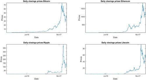
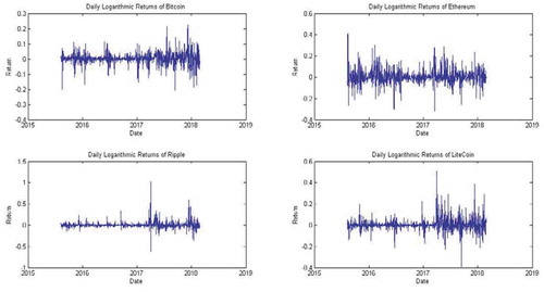
As of February 2020, Bitcoin has a market cap of 175 USD billion representing about 64% of the total cryptocurrency market, followed by Ethereum with a market cap of 29 USD billion representing about 11% of the total market, Ripple with a market cap of 12 USD billion representing approximately 4% of the total market and Litecoin with a market cap of 3.9 USD billion. These four currencies represent approximately 80% of the market capitalization of the total cryptocurrency market, which has a market value of 278.9 USD billion. Historical daily pricing data on Bitcoin, Ethereum, Litecoin, and Ripple are obtained from the website investing.com, which provides long histories of various cryptocurrency exchange rates against the U.S. Dollar (USD). These data range from 8 August 2015 to 25 February 2018. During this period important events have occurred which have been explained in detail in the following paper of Hashemi Joo et al. (2020). We take the daily log returns defined as $R_t=100\times log\left(p_t/p_{t-1}\right)$which can be seen in Figure 2.

Figure 2. Logarithm Return of each cryptocurrency series

The preliminary descriptive statistics of the data are presented in Table 1. Hodrick and Prescott (1997) filter has been used to remove the trend from the log-volume series. As shown in Table 1, the kurtosis of each index is greater than 3 and the skewness is not zero, which both suggest that the presence of fat tails and leptokurtosis. The order for the ARMA part has been chosen, after careful inspection of ACF and PACF of both return and de-trended volume series.

Figure 3. Autocorrelation of Squared Returns

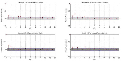
Table 1. Descriptive statistics of the sample data

Descriptive Statistics	Bitcoin	Ethereum	Ripple	Litecoin
observation	933	933	933	933
mean	0.003875	0.0075347	0.005056163	0.00434
std	0.041071	0.07313	0.08096	0.06013
max	0.225119	0.412337	1.02736	0.51035
min	−0.207529	−0.315469	−0.616273	−0.3952
skewness	−0.275847	0.522313	3.1192936	1.45066
kurtosis	8.294972	7.317244	41.5123	16.5257
Jarque-Bera _ 5.9226	1.1006e+003	766.1754	5.9109e+004	7.4e+003
Q(20)_ cv_31.4104	25.4970	36.7330	56.1689	40.2091
ARCH-LM _ 3.8415	50.3921	32.4973	77.4362	20.9612
Adjusted Volume
mean	−0.0000	−0.0000	−0.0000	−0.0000
std	0.469081	0.760698	0.9111	0.73611
skewness	0.521130	0.0732621	0.2169564	0.36286
kurtosis	3.1198463	2.88268776	3.2311953	3.10091
Jarque-Bera	42.7885	1.3696	9.3973	20.8705
Q(20)	2.6395e+003	3.1373e+003	2.5809e+003	3.2e+003
ARCH-LM	282.7823	323.5122	339.7724	332.9092

Notes: Table 1 shows Jarque-Bera is test statistics for the test of normality. Q (20) is the Ljung-Box statistic for serial correlation in the return and adjusted volumes computed with 20 lags. ARCH-LM is the Engel’s LM test for heteroscedasticity, conducted using 20 lags.

*A rejection of the null hypothesis at 5% level

Parameter estimation for return and volume are reported in Table 2. One motivation for using the ARMA-GARCH type model is the inspection of ACF of return and volume and ACF of squared return in Figure 3. After performing the ARCH test over the series of residuals we proceed with the selection of the order of the GARCH model. Here we have applied EGARCH and GARCH type models for return and de-trended volume series, respectively. Further, residuals and squared residuals series do not possess significant autocorrelation for both return and volume series as can be seen in Figure 4 and 5.

Figure 4. ACF of squared standardized residuals of Returns

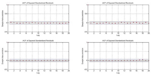
Table 2. Parameter estimation of GARCH and EGARCH model

GARCH for Volume					EGARCH for Returns
Para meters	Bitcoin	Ethe reum	Ripple	Litecoin	Bitcoin	Ethe reum	Ripple	Litecoin
Mean Equation
Μ	−0.0104 (0.0102)	−0.0000 (0.0159)	−0.0233 (0.0179)	−0.0387*** (0.0135)	0.0027*** (0.0005)	0.0000 (0.0015)	−0.0033*** (0.0008)	−0.0000 (0.0005)
ϕ1	0.7566*** (0.0240)	0.7778*** (0.0226)	0.7841*** (0.0207)	0.7961*** (0.0186)	−0.0698** (0.0273)	−0.0114 (0.0336)	−0.0459* (0.0278)	−0.1167*** (0.0223)
Variance Equation
Ω	0.0140*** (0.0069)	0.0000 (0.0000)	0.1471 (0.0932)	0.0048 (0.0035)	−0.0560 (0.0464)	−0.4447 (0.1192)	−0.2607*** (0.0968)	−0.0334* (0.0193)
α1	0.1061*** (0.0351)	0.0198*** (0.0073)	0.0813* (0.0506)	0.0424*** (0.0165)	0.4156*** (0.1164)	0.5374*** (0.0879)	0.9312** (0.5111)	0.2627*** (0.0899)
Β	0.7621*** (0.0833)	0.9793*** (0.0073)	0.4704 (0.3086)	0.9355*** (0.0273)	0.9902*** (0.0068)	0.9159*** (0.0215)	0.9372*** (0.0136)	0.9959*** (0.0033)
γ1	— —	— —	— —	—- —	0.1357** (0.0533)	−0.0197 (0.0442)	−0.1028 (0.1149)	0.1289*** (0.0461)
Ν	12.6094** (5.4331)	53.02 (87.3)	7.7075*** (1.8644)	5.1680*** (0.8592)	2.4064*** (0.2702)	3.2*** (0.4791)	2.0961*** (0.1094)	2.1896*** (0.1240)

Notes:Table 2 reports the estimated parameters for EGARCH and GARCH models for returns and volumes respectively, together with standard errors (in parentheses).

* indicates significance at 10% level.

** indicates significance at 5% level.

*** indicates significance at 1% level.

The test shows that residuals are approximately i.i.d series, therefore copula approach can be applied to the residuals after getting student-t CDF from the residuals. We use the EGARCH and GARCH model to fit the marginal distribution of each return and each volume series. Estimated parameters for each type of model are given in Table 2.

4.2. Marginal distribution models

AR (1)-EGARCH (1,1) models were estimated for all return series by selecting lag order for mean equation by the inspection of ACF and PACF, maintaining the conditional variance equation as EGARCH (1,1) model.

Figure 5. ACF of squared standardized residuals of Volumes

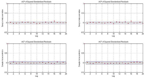
Further, AR (1)-GARCH (1, 1)-t models have been applied to volume series. MATLAB function ’garchfit’ has been used to estimate the parameters of the GARCH and EGARCH models. Parameters estimates can be seen in Table 2. In Table 2, most of the coefficients in the conditional variance equation are significant. Engle’s ARCH test has been applied to the square of the standardized residuals. The test fails to reject the null hypothesis of no ARCH effect.¹

4.3. Copula parameter estimation

We are interested in the dependence structure between the cryptocurrencies’ returns and trading volumes. Our main goal is to explore the extreme dependence between return-volumes and negative return-volume. We employed 6 copulas in our analysis, the first two, namely, Student-t, and Frank copula, are symmetric and they have been used to analyze the dependence structure between each pair of return and volume. The others have been used to analyze the asymmetric dependence between return and volume, as reported in the literature (Karpoff, 1987; Gervais et al., 2001). The asymmetric copulas are able to capture the potential difference between the lower and upper tail. The parameter estimates for each copula have been reported in Table 3 which is based on the Log-Likelihood function.

Table 3. Copula estimates of return-volume dependence

	Bitcoin Ethereum Ripple Litecoin
Student-t copula
ρ	0.0537 (0.0706)	0.0575 (1.453)	−0.0047 (0.1148)	−0.0620 (0.0913)
ν	5.3843*** (1.6130)	100*** (0.0007)	3.9212*** (0.8293)	2.5179*** (0.3609)
AIC	−7.0693	−0.5882	−12.1199	−25.9357
Frank Copula
ρ	0.4000 (.3728)	0.3242 (0.2527)	1.0961 (0.7426)	1.0000e-004 (10.09)
AIC	−0.5661	−0.8215	−0.3595	0.0001
Clayton Copula
ρ	0.2721*** (0.0802)	0.0525 (0.0740)	0.4463 (0.0956)	0.6565 (0.0961)
AIC	−5.3834	−0.2534	−7.7870	−17.4117
Survival Clayton
ρ	0.0980*** (0.0601)	0.0377 (0.0460)	0.1323** (0.0820)	0.0857 (0.0742)
AIC	−1.4990	−0.3547	−1.3008	−0.7124
Gumbel Copula
ρ	1.1000*** (0.0505)	1.1000*** (0.0456)	1.1076*** (0.0536)	1.1000*** (0.0564)
AIC	−0.9150	4.9870	−2.0905	−1.8793
SJC Copula
Upper tail	0.0002 (0.0023)	0.0000 (0.0000)	0.0445 (0.0572)	0.0046 (0.0259)
Lower tail	0.1565*** (0.0605)	0.004 (0.051)	0.2606*** (0.0574)	0.3787*** (0.0461)
AIC	−6.8436	−0.4756	−10.5677	−20.4498

Notes: Table 3 reports the estimates of parameters of six copulas for each pair of return and volume, together with standard errors (in parentheses) and the values of Akaike Information Criteria(AIC).

*** indicates significance at 1% level.

** indicates significance at 5% level

Table 3 exhibits there is no significant symmetric relationship between return and trading volume as evident from the parameter estimates of Student-t and Frank copula for all four currencies. Now we focus on the potential asymmetry in the return-volume dependence by adopting Clayton, Survival Clayton, Gumbel, and SJC copulas. We can see from Table 3 that the parameters of the Clayton and SJC copulas are significant for Bitcoin, Ripple, and Litecoin, which suggest the presence of lower tail dependence. It implies that extremely low returns are associated with low volumes in the case of Bitcoin, Ripple, and Litecoin. Which means during the market stress of cryptocurrencies most of the investor still wanted to keep the cryptocurrencies especially Ripple and Litecoin as compared to Bitcoin.

A possible reason might be that Ripple and Litecoin are cheaper and Bitcoin is expensive. Therefore, during the market stress if the loss is not that much then it is better to wait rather than selling. For someone, Bitcoin proves to be a lottery and someday if it could be true for Ripple and Litecoin to reach the level of Bitcoin might be the reason for low trading volume during market stress.

Further, the new investor always careful in investing during market stress. At the same time, the parameters of the Survival Clayton are significant for all pairs except Ethereum and Litecoin. Further, if we check the parameters of the Gumbel copula, then all the parameters are found to be significant for all pairs of return and volume. The upper tail dependence coefficients for Gumbel and Survival Clayton copula are reported in Table 4, which have been extracted from the EGARCH-Copula model.

Table 4. Extreme dependence Coefficients for returns-volume

	Gumbel		SC		Clayton		SJC
	${\lambda }_{\mathrm{U}}^G$	LL	${\lambda }_{\mathrm{U}}^G$	LL	${\lambda }_L^c$	LL	${\lambda }_L^{SJc}$	LL
Bitcoin	0.1221	−0.9150	0.0009	−1.4990	0.0783	−5.3834	0.1565	−6.8436
Ethereum	0.1221	4.9870	0.0000	−0.3547	0.0000	−0.2534	0.0040	−0.4756
Ripple	0.1302	−2.0905	0.0053	−1.3008	0.2116	−7.7870	0.2606	−10.5677
Litecoin	0.1221	−1.8793	0.0003	−0.7124	0.3479	−17.4117	0.3787	−20.4498

Notes: Table 4 reports the upper tail dependence coefficients, calculated from the Gumbel copula ${\lambda }_U^G=2-2^{1/{\rho }_G}$and Survival Clayton Copula ${\lambda }_U^{SC}=2^{-1/{\rho }_{SC}}$ by taking parameters from Table 3.

We can see from Table 4 that relatively weak upper tail dependence exists in return and volume of the Bitcoin, Ripple, and Litecoin but there is no upper tail dependence existed in Ethereum.

This means that when during the time of market boom there is evidence of trading, but it is not strong evidence according to log-likelihood function. On the other hand, for Ethereum extremely high return and extremely high volume are independent.

Considering no significant relationship between return and volume, which is captured by Student-t and Frank copulas (see Table 3) for all pairs of cryptocurrencies, we also investigated each pair of negative returns and volume to explore whether the extremely high volumes are associated with extremely low returns. The procedure is exactly the same as the one we employed for the return-volume series, the results are reported in Tables 5 and 6. Since the first two copulas have symmetric structure and we just change the sign of returns, the absolute value of the estimated parameters of the elliptic copulas does not change.

Table 5. Copula estimates for negative return-volume dependence

	Bitcoin Ethereum Ripple Litecoin
Student-t copula
ρ	−0.0537 (0.0706)	−0.0575 (1.453)	0.0047 (0.1148)	0.0620 (0.0913)
ν	5.3843*** (1.6130)	100*** (0.0007)	3.9212*** (0.8293)	2.5179*** (0.3609)
AIC	−7.0693	−0.5882	−12.1199	−25.9357
Frank Copula
ρ	0.0001 (0.3661)	0.0001 (0.2501)	0.6920 (1.7225)	1.5283 (0.5600)
AIC	0.0003	0.0005	0.0408	−1.4783
Clayton Copula
ρ	0.0001 (0.0889)	0.0001 (0.0658)	0.3838*** (0.0984)	0.5738*** (0.0974)
AIC	0.0005	0.0020	−4.8962	−11.9307
Survival Clayton Copula
ρ	0.0001 (0.0709)	0.0001 (0.0606)	0.0975 (0.0926)	0.1163 (0.0878)
AIC	0.0017	0.0021	−0.5199	−0.8609
Gumbel Copula
ρ	1.1000*** (0.0518)	1.1000*** (0.0470)	1.1058*** (0.0556)	1.1413*** (0.0547)
AIC	5.1033	11.3945	−1.8298	−3.5921
Symmetrised Joe-Clayton copula
Tu	0.0000 (0.0000)	0.0000 (0.9121)	0.0471 (0.0607)	0.0406 (0.0613)
T_L	0.0557 (166.25)	0.0000 (0.5021)	0.2272*** (0.0583)	0.3362*** (0.0510)
AIC	0.0564	1.4290	−7.4721	−15.7087

Notes: Table 5 reports the estimates of parameters of six copulas for each pair of negative return and volume, together with standard errors (in parentheses) and the values of Akaike Information Criteria (AIC).

***indicates significance at 1% level.

Table 6. Extreme tail dependence coefficients for negative returns-volume

	Gumbel		SC		Clayton		SJC
	${\lambda }_{\mathrm{U}}^G$	LL	${\lambda }_U^{SC}$	LL	${\lambda }_L^c$	LL	${\lambda }_L^{sjc}$	LL
Bitcoin	0.1221	5.1033	0.0000	0.0017	0.0000	0.0005	0.0557	0.0564
Ethereum	0.1221	11.3945	0.0000	0.0021	0.0000	0.0020	0.0000	1.4290
Ripple	0.1284	−0.18298	0.0008	−0.5199	0.1643	−4.8962	0.2272	−7.4721
Litecoin	0.1645	−3.5921	0.0026	−0.8609	0.2988	−11.9307	0.3362	−15.7087

Notes: Table 6 reports the upper tail dependence coefficients, calculated from the Gumbel copula ${\lambda }_U^G=2-2^{1/{\rho }_G}$and Survival Clayton Copula ${\lambda }_U^{SC}=2^{-1/{\rho }_{SC}}$ by taking parameters from Table 5.

Our estimates for Clayton copula and SJC copula in case of negative return-volume are significant except for Bitcoin and Ethereum. This means that extremely low trading volume and extremely high returns show independent behavior for both Bitcoin and Ethereum. However, for Ripple and Litecoin, significant dependence existed between extremely high returns and extremely low volumes, which can be seen from Clayton and SJC copulas estimates from Tables 5 and 6. Which means that even if the market in a boom but running investor still wait for extraordinary profit and the new investor might be scared of consequence. Further Survival Clayton and Gumbel copulas estimated parameters are significant for Ripple and Litecoin. Upper tail dependence coefficients extracted from these two copulas are reported in Table 6, which is, 13% and 16% for Ripple and Litecoin, respectively. This provides evidence that in these two currencies extremely high volumes are likely to be associated with extremely low returns.

In other words, market stress or in crisis is accompanied by high trading volumes. Nevertheless, this is not strong dependence as compared with lower tail dependence parameters of Clayton copula and SJC copula for return-volume series. This says that during crisis volume decreases and the lower tail dependence parameters for Bitcoin, Ripple, and Litecoin are found in Table 6.

This work shows that in the extreme return-volume relationship, extremely higher return and extremely low return are followed by low volume, which evident from the Clayton and SJC copulas tail dependence parameter from Tables 4 and 6 based on log-likelihood function. The leverage effect is referred to as an asymmetric negative correlation between return and volatility. In our study, we found no leverage effect not only from the EGARCH model but also from the return volume dependence. As we have already explained that the volumes are positively associated with volatility, and further extreme low returns are also positively associated with volatility. However, in the case of cryptocurrencies results are contradictory from most of the paper in the literature. Some paper says that if volatility increase then the volume increase and some paper says if the return increase then the volume also increase but both of these are not true in case of cryptocurrencies. We found that in case Ripple and Litecoin higher return and low return are followed by low volume that is new information in case of cryptocurrencies until now. As we Identified that Bitcoin and Ripple are the riskiest cryptocurrencies due to significant lower tail dependence between negative return and volume, which is consistent with the finding of Koo et al. (2020). Further, Naeem et al. (2020) found weaker lower tail dependence for most cryptocurrencies, which is contradictory to our findings.

5. Conclusion and implications

We investigate extreme return-volumes dependence among different cryptocurrencies by employing Copula methodology. We filter out margins by using the EGARCH model for return series and GARCH model for volume series and utilizes them in different copulas in order to measure dependence. Evidence of significant symmetric dependence between return-volume is not found due to insignificance of student-t and Frank copula parameters. In a return-volume relationship, coefficients of lower tail dependence are significant for Bitcoin, Ripple, and Litecoin which means that low returns are followed by low volumes. Lower tail dependence for the return-volume relationship is stronger than the upper tail dependence for Bitcoin, Ripple, and Litecoin. Moreover, for negative return-volume, left tail dependence coefficients are significant for Ripple and Litecoin, which means that high returns are followed by low volumes for Ripple and Litecoin.

In fact, extreme high returns are associated with extreme high trading volumes, but much weakly than for the lower tail. This might be related to heterogeneous crypto-investors, and imply that the arrival of very negative information leads to a fall in returns and trading volumes, whereas the effect of the arrival of very positive information is limited. This finding is unique to the cryptocurrency market, which might be due to the highly volatile nature of cryptocurrencies, with most existing investors holding long positions and not closing them to avoid potential losses, while new investors do not engage in long positions, which leads to lower trading volumes. Our findings are very informative for crypto-traders as they provide insightful information about the dependence between cryptocurrency positive and negative return-volume, especially in the extreme market conditions of cryptocurrencies. Accordingly, crypto-traders can now have a better understanding of the return-volume dependence of high volatility cryptocurrencies, which might make them more able to create trading strategies that exploit the knowledge of trading volumes when trying to predict returns in various market states. The findings are also important for risk management purposes, given that returns and volumes have to be jointly determined while allowing for an asymmetry in the tail dependence.

While we present significant results in this article, data limitation has been a concern in our study. For example, we limited our analysis only to the four largest cryptocurrencies. Also, the cryptocurrency market experienced extreme volatility, potentially classified as a market bubble, from the end of 2017 to the beginning of 2018, and it has been perceived to be a more volatile market than many other markets. Regime switching models could be applied to further study the nature of cryptocurrency returns. Future research could also consider portfolio and hedging analysis within the cryptocurrency markets.

Additional information

Funding

The authors received no direct funding for this research.

Notes on contributors

Muhammad Naeem

Dr. Muhammad Naeem is an Assistant Professor of Financial Mathematics at the UCP Business School at the University of Central Punjab. He holds a PhD in Mathematics for Economics and Financial Applications at “Sapienza” University of Rome, Italy.

He has a keen research interest in asset pricing, energy economics, risk management, econometric modeling, volatility modeling, and emerging financial markets.

This research is also important for risk management purposes, given that returns and volumes have to be jointly determined while allowing for an asymmetry in the tail dependence.

Notes

1. Results of the test will be provided upon request

References

- Akbulaev, P. D. N., & Salihova, S. (2020). The relationship between cryptocurrencies prices and volume. Evidence from bitcoin.
- Attari, M. I. J., Rafiq, S., & Awan, M. H. (2012). The dynamic relationship between stock volatility and trading volume. Asian Economic of PhD Thesis and Financial Review, 2(8), 1085–21.
- Bae, J., Kim, C-J.., & Nelson, C. R. (2007). Why are stock returns and volatility negatively correlated?. Journal of Empirical Finance, 14(1), 41–58. doi:10.1016/j.jempfin.2006.04.005
- Baillie, R. T. (1996). Fractionally integrated model. Journal of Econometrics, 74(1), 3–30. https://doi.org/10.1016/S0304-4076(95)01749-6
- Baillie, R. T., Bollerslev, T., & Mikkelsen, H. O. (1996). fractionally integrated generalized autoregressive conditional heteroscedasticity. Journal of Econometrics, 74(1), 3–30.
- Balcilar, M., Bouri, E., Gupta, R., & Roubaud, D. (2017). Can volume predict Bitcoin returns and volatility? A quantiles-based approach. Economic Modelling, 64, pp.74–81. https://doi.org/10.1016/j.econmod.2017.03.019
- Balduzzi, P., Kallal, H., & Longin, F. (1996). Minimal returns and the breakdown of price-volume relation. Economics Letters, 50(2), 265–269. https://doi.org/10.1016/0165-1765(95)00748-2
- Bollerslev, T. (1986). Generalized Autoregressive conditional heteroscedasticity. Journal of Econometrics, 31(3), 307–327. https://doi.org/10.1016/0304-4076(86)90063-1
- Bouri, E., Lau, C. K. M., Lucey, B., & Roubaud, D. (2019). Trading volume and the predictability of return and volatility in the cryptocurrency market. Finance Research Letters, 29, pp.340–346. https://doi.org/10.1016/j.frl.2018.08.015
- Breidt, F. J., Crato, N., & de Lima, P. J. F. (1998). The detection and estimation of long memory in stochastic volatility. Journal of Econometrics, 83(1–2), 325–348. https://doi.org/10.1016/S0304-4076(97)00072-9
- Brooks, C. (2008). Introductory econometrics for finance. Cambridge University Press, UK. doi:10.1017/CBO9780511841644
- Chen, G., Firth, M., & Rui, 0. M. (2001). The dynamic relation between stock returns, trading volume and volatility. The Financial Review, 38(3), 153–174. https://doi.org/10.1111/j.1540-6288.2001.tb00024.x
- Cherubini, U., Luciano, E., & Vecchiato, W. (2004). Copula method in Finance. John Wiley & Son Ltd.
- Chu, J., Chan, S., Nadarajah, S., & Osterrieder, J. (2017). GARCH modelling of cryptocurrencies. Journal of Risk and Financial Management, 10(4), p.17. https://doi.org/10.3390/jrfm10040017
- Clark, P. (1973). A subordinated stochastic process model with finite variance for speculative prices. Econometrica, 41(No. 1), 135–155. https://doi.org/10.2307/1913889
- Corbet, S., Lucey, B., Urquhart, A., & Yarovaya, L. (2019). Cryptocurrencies as a financial asset: A systematic analysis. International Review of Financial Analysis, 62, pp.182–199. https://doi.org/10.1016/j.irfa.2018.09.003
- Crouch, R. (1970, July-August). The volume of transaction and price changes on the New York Stock Exchange. Financial Analysts Journal, 26(4), 104–109. https://doi.org/10.2469/faj.v26.n4.104
- Demarta, S., & McNeil, A. J. (2005). The t copula and related copulas. International Statistical Review, 73(1), 111–129. https://doi.org/10.1111/j.1751-5823.2005.tb00254.x
- Deng, L., Ma, C., & Yang, W. (2011). Portfolio Optimization via Pair Copula-GARCH-EVT-CVaR Model. Systems Engineering Procedia, 2, 171–181. https://doi.org/10.1016/j.sepro.2011.10.020
- Engle, R. F. (1982). Autoregressive conditional heteroscedasticity with estimates of the variance of United Kingdom inflation. Econometrica, 50(4), 987–1007. https://doi.org/10.2307/1912773
- Epps, T. W., & Epps, M. L. (1976). The stochastic dependence of security price changes and transaction volumes: Implications for the mixture of distributions hypothesis. Econometrica, 44(2), 305–321. https://doi.org/10.2307/1912726
- Floros, C., & Vougas, D. (2007). Trading volume and returns relationship in Greek stock index futures market: GARCH vs. GMM. International Research Journal of Finance and Economics, 12, 98–115.
- Garcia-Jorcano, L., & Muela, S. B. (2020). Studying the properties of the Bitcoin as a diversifying and hedging asset through a copula analysis: Constant and time-varying. Research in International Business and Finance.
- Gervais, S., Kaniel, R., & Mingelgrin, D. (2001). High-volume return premium. The Journal of Finance, 56(3), 877–919. https://doi.org/10.1111/0022-1082.00349
- Goudarzi, H. (2010). Modelling long memory in the Indian Stock Market using fractionally integrated E-garch model. International Journal of Trade, Economics and Finance, 1(3), 231–237. https://doi.org/10.7763/IJTEF.2010.V1.42
- Granger, C., & Morgenstern, O. (1963). Spectral analysis of New York Stock Market prices. Kyklos, 16(1), 1–25. https://doi.org/10.1111/j.1467-6435.1963.tb00270.x
- Gunduz, L., & Hatemi-J, A. (2005). Stock price and volume relation in emerging markets. Emerging Markets Finance and Trade, 41(1), 29–44. https://doi.org/10.1080/1540496X.2005.11052599
- Hashemi Joo, M., Nishikawa, Y., & Dandapani, K. (2020). Announcement effects in the cryptocurrency market. Applied Economics, 1–15. https://doi.org/10.1080/00036846.2020.1745747
- Hodrick, R. J., & Prescott, E. C. (1997). Postwar US business cycles: An empirical investigation. Journal of Money, Credit, and Banking, 29(1), 1–16. https://doi.org/10.2307/2953682
- Jain, P. C., & Joh, G. H. (1988). The dependence between hourly prices and trading volume. The Journal of Financial and Quantitative Analysis, 23(3), 269–283. https://doi.org/10.2307/2331067
- Joe, H. (1997). Multivariate models and dependence concepts. Chapman&Hall.
- Joe, H., & Xu, J. J. (1996). The estimation method of inference functions for margins for multivariate models, Technical Report,166, Department of Statistics, University of British Columbia.
- Jondeau, E., & Rockinger, M. (2006). The copula-GARCH model of conditional dependencies: An international stock market application. Journal of International Money and Finance, 25(5), 827–853. https://doi.org/10.1016/j.jimonfin.2006.04.007
- Kamath, R. R. (2008). The price-volume relationship in the Chilean stock market. International Business and Economic Research Journal, 7, 7–13.
- Kang, S. H., Cheong, C. C., & Yoon, S. M. (2010). Long memory volatility in Chinese stock markets. Physica A, 389(7), 1425–1433. https://doi.org/10.1016/j.physa.2009.12.004
- Kang, S. H., & Yoon, S. (2012). Dual long memory properties with skewed and fat-tail distribution. International Journal of Business and Information, 7, 2.
- Karpoff, J. M. (1987, March). The relation between price change and trading volume: A survey. Journal of Financial Research and Quantitative Analysis, 22(1), 109–126. https://doi.org/10.2307/2330874
- Karpoff, J. M. (1988). Costly short sales and the correlation of return with volume. The Journal of Financial Research, 11(3), 173–188. https://doi.org/10.1111/j.1475-6803.1988.tb00080.x
- Kasman, A., & Torun, E. (2007). Long memory in the Turkish Stock Market return and volatility. Central Bank Review, 13–27.
- Katsiampa, P., Gkillas, K., & Longin, F. (2018). Cryptocurrency market activity during extremely volatile periods. Available at SSRN 3220781.
- Koo, C. K., Semeyutin, A., Marco Lau, C. K., & Fu, J. (2020). An Application of Autoregressive Extreme Value Theory to Cryptocurrencies. The Singapore Economic Review, 1–8. https://doi.org/10.1142/S0217590820470013
- Koutmos, D. (2018). Return and volatility spillovers among cryptocurrencies. Economics Letters, 173, 122–127. https://doi.org/10.1016/j.econlet.2018.10.004
- Kristoufek, L. (2013). BitCoin meets Google Trends and Wikipedia: Quantifying the relationship between phenomena of the Internet era. Scientific Reports, 3(1), 1–7. https://doi.org/10.1038/srep03415
- Kumar, A. (2004). Long memory in stock trading volume: Evidence from Indian Stock Market. Indira Gandhi Institute of Development Research-Economics.
- Kurowicka, D., and Joe, H. (2011). Dependence modeling: Vine Copula handbook. Singapore: World Scientific Publishing Co. doi:10.1142/7699
- Maghyereh, A., & Abdoh, H. (2020). Tail dependence between Bitcoin and financial assets: Evidence from a quantile cross-spectral approach. International Review of Financial Analysis, 71, 101545. https://doi.org/10.1016/j.irfa.2020.101545
- Mashal, R., & Naldi, M. (2002). Pricing multiname credit derivatives:Heavy tailed approach. Quantitative Credit Research Quarterly, 3107–3127.
- MecNeil, A. J., Frey, R., & Embrechts, P. (2005). Concepts, techniques and tools, Quantitative Risk Management. Princeton University Press.
- Naeem, M., Bouri, E., Boako, G., & Roubaud, D. (2020). Tail dependence in the return-volume of leading cryptocurrencies. Finance Research Letters, 36, 101326. https://doi.org/10.1016/j.frl.2019.101326
- Naeem, M., Ji, H., & Liseo, B. (2014). Negative Return-Volume Relationship in Asian Stock Markets: Figarch-Copula Approach. Eurasian Journal of Economics and Finance, 2(2), 1–20. https://doi.org/10.15604/ejef.2014.02.02.001
- Navarro, J. R., Tamangan, R., Guba-Natan, N., Ramos, E., & Guzman, A. D. (2006). The identification of long memory process in the Asian-4 stock markets by fractional and multi-fractional Brownian motion. The Philippine Statistician, 55(1–2), 65–83.
- Nelson, R. B. (2006). An introduction to copulas. Springer-Verlag.
- Ning, C., & Wirjanto, T. S. (2009). Extreme return-volume dependence in East-Asian stock markets: A copula approach. Finance Research Letters, 6(4), 202–209. https://doi.org/10.1016/j.frl.2009.09.002
- Patton, A. J. (2006). modelling asymmetric exchange rate dependence. International Economic Review, 47(2), 527–556. https://doi.org/10.1111/j.1468-2354.2006.00387.x
- Patton, A. J. (2008). Copula toolbox for MATLAB. http://public.econ.duke.edu/ap172/code.html
- Patton, A. J. (2009). Are “market neutral” hedge funds really market neutral?. The Review of Financial Studies, 22(7), 2495–2530 doi:10.1093/rfs/hhn113
- Poyser, O. (2019). Exploring the dynamics of Bitcoin’s price: A Bayesian structural time series approach. Eurasian Economic Review, 9(1), pp.29–60. https://doi.org/10.1007/s40822-018-0108-2
- Puri, T. N. (2008). Asymmetric volume-return relation and concentrated trading in LIFFE Futures. European Financial Management, 14(3), 528–563. https://doi.org/10.1111/j.1468-036X.2007.00396.x
- Rogalski, R. (1978). The dependence of prices and volume. Review of Economics and Statistics, 58(2), 268–274. https://doi.org/10.2307/1924980
- Rossi, E., & Santucci de Magistris, P. S. (2013). Long memory and tail dependence in trading volume and volatility. Journal of Empirical Finance, 22, 94–112 doi:10.1016/j.jempfin.2013.03.004
- Sheppard, K. (2013). Oxford MFE Toolbox. http://www.kevinsheppard.com/wiki/MFE_Toolbox
- Sklar, A. (1959). Fonctions de répartition á n dimensions et leurs marges. Publication De l’Institut De Statistique De l’Universite De Paris, 8, 229–231.
- Sklar, A. (1973). Random variables, joint distribution functions, and copulas. Kybernetika, 9, 449–460.
- Takaishi, T. (2020). Rough volatility of Bitcoin. Finance Research Letters, 32, 101379. https://doi.org/10.1016/j.frl.2019.101379
- Tan, S., & Khan, M. T. I. (2010). Long memory features in return and volatility of the Malaysian Stock Market. Economics Bulletin, 30(No.4), 3267–3281.
- Tang, T. L., & Shieh, S. J. (2006). Long memory in stock index future markets: A value at risk approach. Physica A: Statistical Mechanics and It Applications, 366, 437–448. https://doi.org/10.1016/j.physa.2005.10.017
- Tauchen, G., & Pitts, M. (1983). The price variability-volume relationship on speculative markets. Econometrica, 5, 485–505.
- Tiwari, A. K., Adewuyi, A. O., Albulescu, C. T., & Wohar, M. E. (2020). Empirical evidence of extreme dependence and contagion risk between main cryptocurrencies. The North American Journal of Economics and Finance, 51, p.101083. https://doi.org/10.1016/j.najef.2019.101083
- Urquhart, A. (2017). The volatility of Bitcoin. Available at SSRN 2921082
- Westerfield, R. (1977). The distribution of common stock price changes: An application of transactions time and subordinate stochastic models. Journal of Financial and Quantitative Analysis, 12(5), 743–765. https://doi.org/10.2307/2330254
- Xu, Q., Zhang, Y., & Zhang, Z. (2020). Tail-risk spillovers in cryptocurrency markets. Finance Research Letters, p.101453. https://doi.org/10.1016/j.frl.2020.101453
- Zhang, W., Wang, P., Li, X., & Shen, D. (2018). Multifractal detrended cross-correlation analysis of the return-volume relationship of Bitcoin market. Complexity, 2018.