Redistributive fiscal policies and regional economic disparities

Abstract

Finding a definitive answer to the question of whether fiscal redistribution is harmful or beneficial for regional economic performance is not straightforward. This paper disentangles the key components of fiscal redistribution in a regional Canada-US setting. Redistributive spending is calibrated as the difference between pretax personal income, and personal income after federal taxes and transfers. Based largely on fixed effects and dynamic panel methods, our findings support the battery of studies on the mixed evidence concerning the relationship between fiscal redistribution and per capita income. To the extent that results are sensitive to estimation methods and functional specifications, the study underscores the importance of unbundling the components of a redistributive fiscal package in a bid to establish optimal thresholds for effective policy interventions.

Keywords:

• federalism
• fiscal policies
• redistribution
• regional economy

JEL Classification:

• H3
• H23
• H77
• R11

PUBLIC INTEREST STATEMENT

Redistributive policies have implications for equity, efficiency, and regional development. Most government fiscal transfer programs are based on the relative fiscal capacities of the participating jurisdictions. For instance, compared to US states, Canadian provinces have more flexibility and discretion in the delivery of health, education, and social services. While there is no harmonization in the various state and federal taxing programs, Canada’s fiscal regime is relatively more integrated. Based on the difference between pretax personal income, and personal income after federal taxes and transfers, we investigate the effectiveness of redistributive flows between federal and regional levels of governments. Our results show that finding a definitive answer to the question of whether fiscal redistribution is harmful or beneficial for regional economic performance is not straightforward. We highlight the implications of our findings for policy. While regional fiscal disparity may be bad for growth, policy designs that focus on taxes and transfers may cause more harm than good, because of the complex interactions between different policy instruments.

1. Introduction

Intergovernmental fiscal transfers remain a potent tool for smoothing regional income, in addition to achieving distributional equity. As such, fiscal transfers have consequences, even when they are not a policy objective, ex-ante. This paper examines the relative importance of intergovernmental fiscal redistribution in Canada and the US, two federations with different divisions of powers between national and sub-national governments. The central economic argument for most countries organized along federalist grounds is that economic integration helps maximize efficiency gains from common markets as a result of free trade and factor mobility. At the same time, decentralized decision-making ensures welfare maximization by ensuring that local policies are customized to the needs of often heterogeneous populations with different regional tastes (Kessler & Lessmann, 2008).

Canada and the US share many commonalities in their intergovernmental fiscal regimes, but there are also significant differences. For instance, both federations have two or more orders of government acting directly, rather than through another level of government, on the citizens; and in particular, there is a constitutionally defined distribution of expenditure responsibilities and revenue sources (Boadway & Watts, 2004).

This paper contributes to the literature by disentangling the key components of regional fiscal redistribution in a comparative Canada-US setting. Unlike the US, however, where there is no harmonization in the various state and federal taxing programs, Canada’s fiscal regime is relatively more integrated. For instance, compared to US states, the provinces have more flexibility and discretion in the delivery of health, education, and social services. Also, while Canada’s Equalization program is explicitly intended to redistribute resources among provinces, it has no direct counterpart in the US; the US federal government transfers resources to the states through the Grants-in-Aid system, a much more complex system.

Clearly, the decentralization-growth question remains open, as most cross-country econometric studies provide weak evidence, chiefly because results change depending on the countries examined. Canada and the US are two of the most decentralized fiscal unions in the world. Both federal-provincial and federal-state relations provide for sovereign powers in many areas, including taxing power and the ability to tap all significant sources of revenue, including natural resources.

This paper has two key objectives. By looking at sub-national regions in both countries that share many common characteristics typical of a fiscal union, we control for many jurisdiction-specific features that might obscure the dynamics of the decentralization-growth nexus. Differences in the economic structures and performances among different regions are likely to have an impact on the way fiscal redistribution affects income levels. Using a dynamic panel of Canada-US data, we evaluate the importance of redistributive flows by estimating the relationship between personal income after federal taxes and transfers, and pretax personal income. This gives a direct measure of the degree to which fiscal transfers drive regional incomes. This fulfils the first objective of the study.

Our second objective is to introduce a few refinements in the estimation methods, in a bid to increase the reliability of our econometric estimates. In particular, we make use of the difference and system generalized method of moments (GMM) estimators in a Canada-US sub-national panel data. Most of the latest literature examining the fiscal decentralization-economic growth question tends to rely on cross-country ordinary least squares (OLS) empirical methodology; a few others incorporate the fixed effects model (FEM). An explanatory variable such as net fiscal transfers is going to be endogenous in the model. While this is not the first paper to study the implications of Canada-US interregional fiscal transfers for income convergence, making use of the GMM methods enables us to deal with the implications of endogeneity and unobserved heterogeneity. This is our second major contribution to the literature.

As well, updated results on the impacts of educational attainment and capital stock on sub-national Canada-US income distribution are provided. In the interest of keeping the models and robustness tests as simple as possible, we perform the tests for the baseline model first and compare our results with those obtained from other models. We then offer possible interpretations of the results in light of the estimation strategies employed.

The remainder of the paper is structured as follows. In Section 2, we review related literature. Section 3 discusses theoretical issues related to the growth empirics model, and introduces our data sources and variables. Estimation methods and econometric results are presented in Section 4, while Section 5 concludes with policy lessons.

2. Literature review

2.1. Fiscal redistribution

Arguments for and against decentralization abound in the literature. Public finance theory posits that fiscal decentralization helps to increase the degree of efficiency in the allocation of resources: lower levels of governments are closer to the people and are believed to have an informational advantage on the needs and preferences of residents, compared to central governments (Ezcurra & Rodríguez-Pose, 2009). When factor mobility advantages accrue as a result of fiscal decentralization, such efficiency gains will generate further benefits through the domino effect.

As a pre-condition for economic convergence, for instance, fiscal transfers to poorer regions will be needed to help finance the investment needed to raise the productivity levels of residents of these regions. On the other hand, some sub-national governments may not have the capacity and sophistication required to make optimal decisions on resource allocation, compared to the central government (Gill & Rodríguez-Pose, 2004). Also, fiscal transfers may supplement the income of regions with low productivity due to adverse climatic conditions or other geographic disadvantages.

On Equalization transfers, for instance, Canadian territories receive more on a per capita basis than the provinces, due to the harsher climatic conditions and remoteness of the territories. This explains, partly, why the territories are sparsely populated, resulting in high costs of public services. Climate and remoteness are a source of disincentive for labour mobility, and this explains why convergence in productivity, as predicted by theory, often does not happen. Regardless, such transfers can be justified on equity grounds (Boadway & Flatters, 1982). Likewise, employment insurance plays a significant role in transferring income to regions with high unemployment; rules are designed to make qualification easier in high unemployment regions.

While the nature of the relationship between fiscal decentralization and economic growth continues to attract considerable attention in the literature, the direction of this relationship remains an open question. Some empirical tests show a negative or no relationship at all, e.g., Davoodi and Zou (1998), Zhang and Zou (1998), Woller and Phillips (1998), and Xie et al. (1999). Others, such as Lin and Liu (2000), Akai and Sakata (2002), and Stansel (2005), establish a positive association. One important consensus in the literature remains: the degree of fiscal decentralization is important in the growth process of any nation.

Bayoumi and Masson (1993) shed light on why a federal system may tend to support a redistributive fiscal regime. First, they claim to the extent that taxes are higher in regions with high incomes, redistribution will help achieve regional after-tax income equalization. The fact that corporate taxes are, to a large extent, related to income, is their second premise. Political considerations and the fact that poor regions are often in more social need (meaning residents receive personal transfer payments to help in poverty alleviation) are the other justifications provided by Bayoumi and Masson.

Thieβen (2005) posits that there exists an inverted U-shaped relationship between fiscal decentralization and economic growth in the OECD countries. This means a quadratic specification¹ is required to estimate the optimal level of fiscal transfers required to maximize economic growth. A positively sloped curve arises when fiscal decentralization increases from low levels, while any additional transfers beyond the optimum result in a negatively sloped curve.

2.2. Fiscal transfers and growth empirics

One of the main predictions of the neoclassical growth model is that less affluent regions will grow faster than more affluent ones, provided the different regions are at different points relative to their steady state growth paths (Solow, 1956; Swan, 1956). This has become known as beta-convergence; for instance, Barro (1991), Barro and Sala-i-Martin (1991; 1992), Mankiw et al. (1992), and Sala-i-Martin (1996) provide empirical evidence of income convergence of approximately 2% per annum for regions of the US, Japan and Europe.

Bayoumi and Masson (1993) use fiscal transfers at the sub-national level within the US and Canada to analyze long-term fiscal flows (the redistributive element) and short-term responses to regional business cycles (the stabilization element). While long-run flows amount to 22 cents of every dollar spent while the stabilization effect is 31 cents in the dollar for the US, Canada produces a larger redistributive effect (39 cents) and smaller stabilization effect (17 cents). They conclude that federal flows appear to depend on the institutional structure of the country concerned, in addition to providing evidence that a federal fiscal system tends to support the relative income of poor regions, compared to rich ones.

Akai and Sakata (2002) provide evidence that fiscal decentralization contributes to economic growth, using state-level data drawn from an economic survey of the US that leaves out a period of high economic growth. Though consistent with theoretical results, their finding contradicts the empirical results of many papers before theirs. Akai and Sakata (2002) allude their finding to the nature of the data set used in the regression analysis. Among other things, this data set is characterized by small differences in history, culture, and the stage of economic development. They admit that such distortion-free data set did indeed reveal the true positive effect of fiscal decentralization. Akai and Sakata conclude that in measuring the impact of fiscal decentralization on economic growth, it is important to get the definition of fiscal decentralization right.

Using a system of simultaneous equations, Checherita et al. (2009) use a large sample of European regions covering 19 European Union (EU) member states for the 1995–2005 period to analyze the aggregate impact of taxation and transfers on income and output convergence. They find evidence in support of a convergence process across the member states in terms of both per-capita output and income. Their results show that, on average, net fiscal transfers impede output growth. Output growth rates in less prosperous receiving regions decline by less, compared to contributing more prosperous regions, in reaction to the fiscal transfers: a condition termed immiserising convergence.

Bargain et al. (2013) study the redistributive and stabilizing effects of a fiscal equalization scheme in the Euro area. They examine the economic effects of introducing the following two elements of a fiscal union, using representative household micro data from 11 Eurozone countries: (i) an EU-wide tax and transfer system, and (ii) an EU-wide system of fiscal equalization. Their study reveals huge redistributive consequences—both within and across countries—after replacing one third of the national tax and transfer systems by a European system. While they conclude that the EU system will benefit credit-constrained countries in particular, through improved fiscal stabilization, their work also suggests that a fiscal equalization regime based on taxing capacity will lead to income redistribution from high- to low-income countries—with ambiguous stabilization properties.

Using dynamic panel data (DPD) techniques, Potrafke and Reischmann (2014) ask whether fiscal policy conducted by sub-national governments in Germany and the US is based on fiscal transfers. Employing a Bohn-type (Bohn, 1998) fiscal reaction function, and based on the assumption that the debt-to-GDP ratio in the preceding period has a positive influence on the primary surplus-to-GDP ratio in the current period, they find that sustainable fiscal policy in the US and Germany is only achievable through fiscal transfers.

McInnis (1968), the pioneer of studies on regional disparities in Canada, uses per capita income levels for the provinces (relative to the Canadian average) in both weighted and non-weighted terms to show that the income gap from 1926 to 1962 stayed the same. On the US side, Barro and Sala-i-Martin (1990) use a neoclassical growth framework to establish the presence of β-convergence across US states. They find a rate of about 2–2.5% per annum between 1940 and 1988 for per capita personal income and between 1963 and 1988 for per capita gross state product. Six years after, Sala-i-Martin (1996) included Japanese prefectures, regions in Western Europe, and Canadian provinces. Results show income convergence rates of 2.4% from 1961 to 1991 for Canada; 1.5–1.8% from 1950 to 1990 for Western Europe; 1.9–3.1% from 1955 to 1990 for Japan; and 1.7–2.2% from 1880 to 1990 for the US.

3. Data, theoretical setup, and model specification

3.1. Data sources

Our data are compiled from the following sources: US Bureau of Economic Analysis (Regional Economic Accounts), Statistics Canada (Provincial Economic Accounts), World Bank (National Accounts Data), OECD (National Accounts Data Files), and the Bank of Canada (Rates and Statistics—Annual Average Exchange Rates.

We exploit a panel data set spanning eight three-year intervals from 1987² to 2010, and covering all 10 Canadian provinces and 50 states of the US. This gives rise to N = 60; T = 8. In the regression analysis, T becomes 7 because we lose one time period due to the lagged per capita real GDP. Hence, we have 420 observations. Real GDP per capita data are obtained from the Regional Economic Accounts and Provincial Economic Accounts. Canadian data are converted into US dollars using annual Canada-US average nominal exchange rates. Relative per capita GDP is constructed as the ratio of the per capita GDP of a province (state), relative to the Canadian (US) average.

3.2. Theoretical setup

We base our analysis on the empirics of economic growth. A framework to test the Solow growth model is the growth empirics method of Mankiw et al. (1992), who extend the Cobb-Douglas formulation of Solow’s growth model to include human capital, as well as physical capital. This implies an underlying aggregate production function of the form:

(1) ${\mathrm{Y}}_{\mathrm{j}\mathrm{t}}={\mathrm{K}}_{\mathrm{j}\mathrm{t}}^{\alpha }{\mathrm{H}}_{\mathrm{j}\mathrm{t}}^{\beta }{\left({\mathrm{A}}_{\mathrm{j}\mathrm{t}}{\mathrm{L}}_{\mathrm{j}\mathrm{t}}\right)}^{1-\alpha -\beta }$(1)

where Y is total income, L is labour supply, and A is a technology parameter, with L growing at an annual rate n and A growing at rate g. In line with Solow, Mankiw et al. (1992) rewrite income, physical capital, and human capital in (1) in terms of quantities per unit of effective labour:

(2) $y_t=\frac{Y_t}{A_t{L}_t}$(2)

(3) $k_t=\frac{K_t}{A_t{L}_t}$(3)

(4) $h_t=\frac{H_t}{A_t{L}_t}$(4)

The changes over time in physical and human capital per unit of effective labour are:

(5) ${\dot{k}}_t=s_k{y}_t-\left(n+g+\delta \right)k_t$(5)

where δ is the rate of depreciation for both physical and human capital, and $s_k$ and $s_h$ are the savings rates for physical and human capital, which are assumed to be constant over time, though not across countries.

Solving for steady-state solutions k* and h*, Mankiw et al. (1992) derive an equation for steady-state income growth as follows:

(6) $\mathrm{l}\mathrm{n}{\mathrm{Y}}_{\mathrm{t}}=\mathrm{l}\mathrm{n}{A}_0+g_t-\left(\frac{\alpha +\beta }{1-\alpha -\beta }\right)ln\left(n+g+d\right)+\left(\frac{\alpha }{1-\alpha -\beta }\right)\mathrm{l}\mathrm{n}{s}_k+\left(\frac{\beta }{1-\alpha -\beta }\right)\mathrm{l}\mathrm{n}{s}_h$(6)

The physical capital savings rate, $s_k$, was approximated by the investment share in GDP, while the human capital savings rate, $s_h$, was measured by the proportion of the working age population at any one time enrolled in secondary school. Mankiw et al. (1992) conclude that augmenting the Solow model with measures of human capital leads to an improvement in its predictive power of explaining cross-country per capita output growth and levels.

3.3. Model specification

The econometric specification below captures the dependence of real GDP per capita on fiscal transfers and other control variables:

(7) $\begin{array}{rl}& \mathrm{l}\mathrm{n}\mathrm{R}\mathrm{G}\mathrm{D}{\mathrm{P}}_{it}={\beta }_0+{\beta }_1\left(lnRGD{P}_{it-1}\right)+{\beta }_2\left(NF{T}_{it}\right)+{\beta }_3\left(NFT.lnRGD{P}_{it-1}\right)\\ & +{\beta }_4(\mathrm{E}\mathrm{D}{\mathrm{U}}_{\mathrm{i}\mathrm{t}})+{\beta }_5\left(CA{P}_{it}\right)+\mathrm{J}\mathrm{U}{R}_i+TI{M}_t+{\mu }_{\mathrm{i}\mathrm{t}}\end{array}$(7)

All variables and notations are defined below:

$RGD{P}_{it}$ Real GDP per capita for jurisdiction i at time t

$NF{T}_{it}$Net fiscal transfers for jurisdiction i at time t

$ED{U}_{it}$Human capital stock for jurisdiction i at time t

$CA{P}_{it}$Physical capital stock for jurisdiction i at time t

$JU{R}_i$Jurisdiction-specific effects

$TI{M}_t$Year-specific effects

${\mu }_{it}$Random error term for jurisdiction i at time t.

3.4. Variables

Most government fiscal transfer programs are based on the relative fiscal capacities of the participating jurisdictions. In Canada, the Equalization program is executed based on a formula-driven measure of provincial fiscal disparities. Provinces with relatively low fiscal capacities receive the most transfers on a per capita basis, while provinces with high fiscal capacities receive less. Not just that, the program is set up such that as a province’s relative fiscal capacity grows, the new program automatically reduces fiscal transfers and vice versa.³ On the other hand, the US is one of the few federations in the world without a formal system of equalization, designed to reduce fiscal disparities, among its sub-national governments. However, it uses its other federal grants programs in such a way that the relative fiscal capacities of states are taken into consideration.

For instance, Medicaid, the largest states’ federal grants program is implemented on the basis of the formula based “Federal Medicaid Assistance Percentages” or FMAP (Stark, 2010). The FMAP formula uses relative per capita income as a measure of fiscal capacity. This percentage is calculated by reference to the relative per capita income of states—thereby guaranteeing higher FMAP for low-income states and lower FMAP for high-income states (Stark, 2010). Similarly, under the Canadian Equalization program, once a province is deemed to have adequate fiscal capacity to provide essential public services, it stops being a beneficiary of the program.

The Bureau of Economic Analysis defines personal income as the income received by residents from participation in production, from government and business transfer payments, and from government interest. Statistics Canada uses a slightly different definition: personal income is defined as the sum of all incomes received by residents, including returns for labour and investments, and transfers from the government and other sectors (including old age security payments and employment insurance). In essence, personal income⁴ includes both earnings and transfers such as wages and salaries, supplementary labour income, dividends, interest and miscellaneous investment income, and all transfer payments. Personal disposable income is what is left from personal income after deducting direct taxes and other mandatory insurance premiums to government.

3.5. Net fiscal transfers

Following Bayoumi and Masson (1993), Obstfeld and Peri (1998), and Checherita et al. (2009), our net fiscal transfers variable is constructed as net transfers (i.e., the difference between personal income and disposable income) as a percentage of personal income:

(9) $\mathrm{N}\mathrm{F}{\mathrm{T}}_{it}=\left(\frac{\mathrm{R}\mathrm{P}\mathrm{I}{ }_{it}-\mathrm{R}\mathrm{P}\mathrm{D}\mathrm{I}{}_{it}}{\mathrm{R}\mathrm{P}\mathrm{I}{ }_{it}}\right)$(9)

Here, $\mathrm{R}\mathrm{P}{\mathrm{I}}_{it}$ is real personal income per capita, and $\mathrm{R}\mathrm{P}\mathrm{D}{\mathrm{I}}_{it}$ is real personal disposable income per capita. $\mathrm{N}\mathrm{F}{\mathrm{T}}_{it}$, therefore, represents the percentage of income that constitutes the transfers. This ratio reflects the distributional outcomes of net taxes, and transfers paid and received by households in a region (Obstfeld & Peri, 1998). The difference between the two gives a fair approximation of the redistributive policy in a federal system.

As part of our robustness checks, we also use relative fiscal transfers as an alternative measure of fiscal transfers. In this case, both $\mathrm{R}\mathrm{P}\mathrm{I}{ }_{it}$and $\mathrm{R}\mathrm{P}\mathrm{D}\mathrm{I}{ }_{it}$ are constructed as the ratio between each province (state), relative to the Canadian (US) average—as discussed above. We also use personal current transfer receipts as an alternative fiscal transfers measure. The US Bureau of Economic Analysis defines this variable as the benefits received by persons for which no current services are performed. In other words, payments by governments and businesses to individuals and nonprofit institutions serving individuals.

3.6. Human capital

Human capital stock is one of the two control variables employed in the model. We use educational attainment, $ED{U}_{it}$, as a proxy for human capital; this is defined as the percentage of persons 25 years and over who have completed at least a Bachelor’s degree. Data on educational attainment for all Canadian provinces come from Statistics Canada’s Labour Force Survey (LFS), CANSIM Table 282–0004. Corresponding educational attainment data for all 50 US states are obtained from the US Census Bureau, American Community Survey (ACS). ACS provides estimates of educational attainment for US states on an annual basis from 2000 onwards; prior to this time, only 1990 data are available. Hence, we interpolate the earlier data.

3.7. Physical capital

Physical capital stock is our proxy for investment in infrastructure. We use gross private capital as a percentage of GDP for US states, and gross business fixed capital formation as a percentage of GDP for Canadian provinces. Following Yamarik (2011) and Hall and Jones (1999), we construct our capital stock series using the perpetual inventory method (PIM):

(10) $K_t=K_{t-1}-\delta K_{t-1}+GF{K}_t=\left(1-\delta \right)K_{t-1}+GF{K}_t$(10)

where K_t is capital stock level at time t, GFK_t is gross fixed capital formation at time t, and δ is the rate of depreciation (which is assumed to be constant over time). To implement the PIM, the size and time profile of depreciation rates, gross investment time series, and an initial level of capital stock are required. We construct the initial capital stock using Hall and Jones’ formula:

(11) $K_0=\frac{GF{K}_0}{\delta +g_{GFK}}$(11)

where K₀ is the initial capital stock, GFK₀ is the level of gross fixed capital formation in the initial period, $g_{GFK}$ is the average annual geometric growth rate of GFK, and δ is as previously defined. We assume that capital stocks depreciate at a constant rate of 6%, in line with Hall and Jones.

Canadian provincial capital stock data are calculated using the PIM discussed above, with data on business gross fixed capital formation—the private sector portion of total GFK. We use GFK data for estimating the initial capital stock. Our $g_{GFK}$ value⁵ is taken as 3.6%—based on the average of Statistics Canada’s old and new capital stock annual growth rates. Equivalent capital stock data for US states are based on Yamarik’s net private capital stock data⁶ constructed for the 50 states. Since Yamarik’s data are available only up to 2007, we assume that capital stock and GDP grew at the same rate for the 2008–2010 period. We therefore use the growth rates of real GDP to derive the capital stock figures for 2008, 2009, and 2010.

3.8. Econometric strategy

Our strategy employs, and compares, four econometric methods for estimating the specified model: OLS, FEM, difference GMM, and system GMM. A number of specifications are used to test the central hypotheses, using the Solow Growth model as the benchmark, and our results are compared with those of pioneers in this area, e.g., Bayoumi and Masson (1993), and Checherita et al. (2009). By looking at jurisdictions that share many common characteristics, we empirically model various scenarios, while leveraging the GMM methodology to control for endogeneity and many country-specific features that might obscure the influence of key variables. In all specifications, we apply both least squares and panel estimation techniques, in addition to the difference and system GMM estimators. Different scenarios on instruments exogeneity and functional forms are modeled separately as part of our robustness checks.

3.9. OLS and FEM

While the OLS strategy is expected to generate upward biased estimates, due to its inability to incorporate the panel structure of the datasets, the FEM does handle the panel framework well, albeit it produces downward-biased estimates because it is unable to handle the dynamic component, which involves the lagged dependent variable and regression residuals.

Given the inclusion of the lagged value of the income variable in our growth empirics framework, traditional panel data estimators, such as fixed and random effects, will not be consistent. The FEM is inconsistent because it often eliminates the error term by a de-meaning transformation that induces a negative correlation between the transformed error and the lagged dependent variables of order 1\T, which in short panels remains substantial (Cavalcanti et al., 2012).

3.10. Difference and system GMM

The difference GMM methodology seamlessly captures the lagged endogenous variable as an explanatory variable by first-differentiating the regression each period in order to eliminate individual specific effects. The system GMM on the other hand incorporates both lagged levels and lagged differences. This estimator is obtained at a cost involving a set of additional restrictions on the initial conditions of the process generating y (Baum, 2013).

We also can no longer impose the restriction that there is no correlation between the error term and the explanatory variables required for random effects consistency. Any traces of heteroscedasticity or serial correlation in the errors will render the estimators inconsistent. We therefore rely on the Arellano-Bond strategy in estimating a GMM model set up as a system of equations, one for each time period. That way, different instruments relate to a different equation (Arellano & Bover, 1995; Blundell & Bond, 1998; and Baum, 2013).

Blundell and Bond’s argument essentially points to the fact that with a finite sample size, the first-differenced GMM estimator could lead to biased results since the reliability of ${\mathrm{Y}}_{\mathrm{i}\mathrm{t}-1}$ and ${\mathrm{Y}}_{\mathrm{i}\mathrm{t}-2}$ as instruments cannot be guaranteed when real GDP per capita, net fiscal transfers, and openness are continuous. Arellano and Bover (1995) and Blundell and Bond (1998) show that the system GMM estimator generates good instruments by combining the standard set of equations with an additional set of equations in levels, with lagged differences used as instruments for the levels equations.

To summarize, we employ and compare four econometric methods for estimating the specified models. We start with OLS to provide a benchmark for the other approaches, and then proceed to FEM, before employing the difference GMM and system GMM.

3.11. Descriptive and exploratory analysis

Canada and the US are two affluent countries. However, the various provinces and states that make up both countries are characterized by large income gaps, growth differentials, and differences in fiscal capacities.

Figure 1 shows the regional income distribution in Canada and the US (with Mexico for context. The relatively affluent nature of the US and Canada (compared to Mexico) is amplified by Figure 1’s varying colour shades—almost entirely red and orange for Mexico; different shades of green for Canada and the US. Table 1 corroborates the income distribution pattern displayed in Figure 1. As depicted, all US and Canadian jurisdictions have real GDP per capita greater than 25,000 USD.⁷

Figure 1. Income distribution in Canada, US, and Mexico (2008)

Source: Statistics Canada, US Census, and Reddit.com

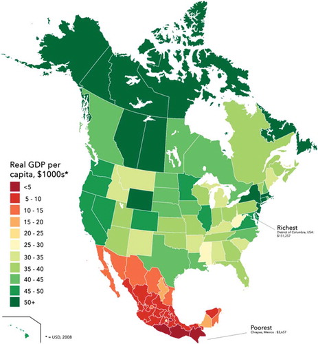
Table 1. Per capita income levels for US and Canadian jurisdictions (2007–2010)

Panel A: Top five jurisdictions
Jurisdiction	Per capita income ($)		Jurisdiction	Per capita income ($)
Alaska	68,847		Alberta	66,080
Wyoming	67,929		Newfoundland	50,438
Connecticut	64,997		Saskatchewan	48,789
Delaware	62,587		Ontario	42,348
Massachusetts	59,756		British Columbia	41,846
Panel B: Bottom five jurisdictions
Jurisdiction	Per capita income ($)	Jurisdiction		Per capita income ($)
Mississippi	31,744	Prince Edward Island		31,277
West Virginia	34,496	Nova Scotia		34,787
Idaho	35,567	New Brunswick		34,903
Arkansas	35,612	Quebec		37,126
South Carolina	35,880	Manitoba		39,689

Notes: Figures in Panel A are in descending order; figures in Panel B are in ascending order. Data are averaged over the 2008–2010 period. Per capita income is based on real GDP as explained under the data section.

At 68,847 USD and 66,080, USD, Alaska and Alberta come first on our per capita income ranking for each country (Table 1 Panel A). Prince Edward Island and Mississippi rank as the poorest jurisdictions in their respective countries, with 31,277 USD and 31,744 USD in average incomes, over the 2007–2010 period. From Table 1, the richest and poorest US states are richer than their Canadian counterparts. The table also shows that there are large regional income gaps between the richest and poorest jurisdictions in the US and Canada. This has important policy implications.

Fiscal decentralization is at the heart of the discussion on whether poor regions eventually catch-up with affluent ones, and how long this might take. The richest state and province, Alaska and Alberta, respectively, are resource-endowed jurisdictions with sole access to natural resource revenues, which have greatly enhanced their fiscal capacities over the years. This is also the case for jurisdictions like Wyoming, Saskatchewan, Newfoundland, and North Dakota, all with above average incomes (Table 1). Natural resources continue to play an important role in these countries’ overall economic picture. Bernard (2012) observes this, and concludes that the large differences in revenues obtained by the resource-endowed jurisdictions and the instability of resource prices have been—and remain—some of the greatest difficulties encountered in the implementation of the Canadian Equalization program.

The observed distribution in average income above can be attributed, at least partly, to fiscal federalism. Sub-national governments in fiscal unions receive significant transfers from the central government, in different forms, to assist them in the provision of essential programs and services. The Canadian Constitution specifically makes provision for Equalization to ensure the regions have the fiscal capacity to provide reasonably comparable levels of public service at reasonably comparable levels of taxation. The US does not have such a system; its closest intergovernmental fiscal transfer mechanism is the Grants-in-Aid system, which the US federal government uses to extend aid to the states and local governments to finance certain areas of domestic public spending. To continue to qualify for federal funds for projects, recipients have to abide by certain rules from the federal government. The Grants-in-Aid system has grown steadily for more than a century; Stark (2010) suggests the adoption of a Canada-type Equalization as a strategy to address the huge fiscal disparities among the states of the US.

Net fiscal transfers (NFT) and relative net fiscal transfers (RNFT) are both expressed as a percentage of primary income. Table 2, sorted on the basis of both NFT and RNFT, shows that the US state of Connecticut (with −14.2% NFT and −4.5% RNFT) and the Canadian province of Alberta (−17.3% NFT and −5.7% RNFT) emerge as the highest contributors (Panel B). Negative transfers from these jurisdictions imply that they are net contributors to the fiscal redistributive regimes in each country. Tennessee (−6.9% NFT and 3.7% RNFT) and Newfoundland (−2.4% NFT and 11.3% RNFT) are the top net fiscal recipients (Panel A). The picture that emerges in Table 2 does not come as a surprise, especially when reconciled with our earlier discussion on sub-national income distribution in Table 1. Poor jurisdictions are, on average, more likely to be net recipients, while rich jurisdictions are more likely to be net contributors.⁸

Table 2. Net fiscal transfers for US and Canadian jurisdictions (2007–2010)

Panel A: Top five jurisdictions
Jurisdiction	NFT (%)	RNFT (%)	Jurisdiction	NFT (%)	RNFT (%)
Tennessee	−6.9	3.7	Newfoundland	−2.4	11.3
South Dakota	−7.0	3.6	Prince Edward Island	−2.5	11.2
Mississippi	−7.4	3.1	New Brunswick	−4.6	8.8
New Mexico	−8.1	2.4	Nova Scotia	−7.4	5.6
Texas	−8.2	2.2	Manitoba	−10.5	2.1
Panel B: Bottom five jurisdictions
Jurisdiction	NFT (%)	RNFT (%)	Jurisdiction	NFT (%)	RNFT (%)
Connecticut	−14.2	−4.5	Alberta	−17.3	−5.7
New York	−13.9	−4.1	Ontario	−12.9	−0.7
Massachusetts	−12.7	−2.8	British Columbia	−11.1	1.4
New Jersey	−11.9	−1.9	Quebec	−11.0	1.5
Maryland	−11.7	−1.6	Saskatchewan	−10.5	2.1

Notes: Figures in Panel A are in descending order; figures in Panel B are in ascending order. Data are averaged over the 2007–2010 period. NFT stands for net fiscal transfers; RNFT for relative net fiscal transfers.

Another interesting observation from Table 2 is that Newfoundland received more than Tennessee, both in absolute and relative terms. The converse is true for Alberta and Connecticut: the former contributed more than the latter both in absolute and relative terms. This underscores the greater redistribution of the intergovernmental fiscal policy in Canada, compared to the US.

4. Estimation results and discussion

Table 3 presents the results. In column [1], OLS returns a coefficient value of 0.955 for ${\mathrm{Y}}_{\mathrm{i}\mathrm{t}-1}$, whereas the FEM returns a coefficient value of 0.524.⁹ We use both versions of the GMM estimator: the difference GMM (DGMM) and system GMM (SGMM) estimators. The coefficient for the lagged dependent variable under DGMM is similar to that under FEM, but much closer to the OLS result, under SGMM.

Table 3. Estimation results (dependent variable: ln RGDP_t)

	[1]	[2]	[3]	[4]
Estimation method	OLS	FEM	DGMM	SGMM
$lnRGD{P}_{t-1}$	0.955***	0.524***	0.547***	0.958***
	[0.019]	[0.083]	[0.100]	[0.031]
$NFT$	−0.019	−2.263***	−2.286***	−0.037
	[0.146]	[0.384]	[0.444]	[0.193]
$lnRGD{P}_{t-1}\times NFT$	−0.073	−0.292	−0.302	−0.195
	[0.263]	[0.990]	[1.072]	[0.412]
Capital stock	0.018*	−0.035*	−0.042**	0.017
	[0.007]	[0.019]	[0.020]	[0.014]
Educational attainment	0.092*	0.318	0.087	0.073
	[0.050]	[0.303]	[0.365]	[0.108]
Year fixed effects	Yes	Yes	Yes	Yes
Number of jurisdictions	60	60	60	60
Observations	360	360	300	360
R-Squared	0.962	0.556
Instruments			91	119
Sargan Test (p value)			0.000	0.000
Hansen Test (p value)			0.995	1.000
Arellano-Bond AR(1) (p-value)			0.019	0.003
Arellano-Bond AR(2) (p-value)			0.659	0.502

Notes: Figures in parentheses are robust standard errors. * significant at 10%; **significant at 5%; ***significant at 1%; no sign means not significant at 1%, 5%, and 10%. All estimations based on the Windmeijer’s (2005) finite sample correction to the standard errors.

Under the FEM and DGMM estimators, the coefficients on relative net fiscal transfers are negative and statistically significant at the 1% level. They are also negative under OLS and SGMM, albeit not statistically significant. This provides evidence for the negative effect of fiscal transfers on per capita income. The interaction terms between lagged per capita GDP and fiscal transfers are not statistically significant under the four scenarios modeled. This has a major implication.

Educational attainment is positively associated with per capita GDP, but significantly so only under OLS. Similarly, capital stock is positively and significantly related to per capita GDP only under the OLS model. This positive association disappears under FEM, DGMM, and SGMM, and in fact, becomes significantly negative instead, under FEM and DGMM. Although this does not align with the predictions of the Solow growth model, it may be that the effect of capital on per capita GDP is absorbed by the other variables in the model.

Table 4 reports the outcomes for the SGMM model only, with results from the third to the seventh lags included for clarity.

Table 4. Two-step system GMM (dependent variable:: ln RGDP_t)

	[1]	[2]	[3]
$lnRGD{P}_{t-1}$	1.041***	0.964***	1.078**
	[0.064]	[0.070]	[0.504]
$NFT$	0.121	0.875***	−1.408
	[0.211]	[0.254]	[3.853]
$lnRGD{P}_{t-1}\times NFT$	0.203	3.148	−0.862
	[0.691]	[2.014]	[3.518]
Capital stock	−0.013	0.059**	−0.063
	[0.026]	[0.026]	[0.381]
Educational attainment	−0.171	0.439	−2.082
	[0.223]	[0.305]	[5.286]
Year fixed effects	Yes	Yes	Yes
Number of observations	360	360	360
Number of jurisdictions	60	60	60
Number of lags used	3&4	5&6	6&7
Number of instruments	54	25	13
Sargan Test (p value)	0.002	0.000	0.681
Hansen Test (p value)	0.234	0.204	0.587
Arellano-Bond AR(1) (p-value)	0.002	0.004	0.131
Arellano-Bond AR(2) (p-value)	0.334	0.283	0.392

Notes: Figures in parentheses are robust standard errors. * significant at 10%; **significant at 5%; ***significant at 1%; no sign means not significant at 1%, 5% and 10%. All estimations based on the Windmeijer’s (2005) finite sample correction to the standard errors.

All three specifications include the same variables, and the only difference between specifications is that column [1] is based on third and fourth order lags, column [2] is based on fifth and sixth order lags, while column [3] is based on sixth and seventh order lags.¹⁰

The estimated lagged real per capita GDP coefficient is somewhat sensitive to the choice of lag length. For instance, going from the fifth and sixth to the sixth and seventh lags leads to an increase in the coefficient on the lagged dependent variable from 0.964 to 1.078. Similar to the lagged dependent variable, the coefficients on net fiscal transfers and capital stock also become statistically significant at the 1% level in column [2]. However, contrary to the results in Table 3, the coefficient signs indicate that net fiscal transfers increase per capita GDP, as does capital stock. That is, net fiscal transfers raise per capita incomes in those jurisdictions that receive them. Across all specifications, the coefficients on the interaction term, and on educational attainment, are not significant.

4.1. Sensitivity analysis

As discussed under data/variables, a concern with this work is that variable definitions could affect results. We therefore examine the robustness of our results to alternative measures of net fiscal transfers. To do this, we define fiscal transfers as personal current transfer receipts, and assume that this variable is endogenous and instrumented using the standard GMM instruments. Results are presented in Table 5.

Table 5. Personal current transfer receipts (dependent variable:: ln RGDP_t)

	[1]	[2]	[3]	[4]
Estimator	OLS	FEM	SGMM1	SGMM2
$lnRGD{P}_{t-1}$	0.866***	0.166	0.726***	−0.591
	[0.080]	[0.230]	[0.175]	[0.969]
$PCT$	−0.002	−0.312***	0.006	0.166
	[0.017]	[0.071]	[0.038]	[0.107]
$lnRGD{P}_{t-1}\times PCT$	0.084	0.427*	0.209	1.509
	[0.073]	[0.245]	[0.168]	[0.947]
Capital stock	0.020***	−0.004	0.022***	0.066***
	[0.007]	[0.021]	[0.008]	[0.018]
Educational attainment	0.068	0.185	0.065	0.050
	[0.048]	[0.092]	[0.66]	[0.171]
Year fixed effects	Yes	Yes	Yes	Yes
Number of observations	360	360	360	360
Number of jurisdictions		60	60	60
Number of instruments			100	16
Number of lags used			0+	5+
R-squared	0.960	0.421
Sargan Test (p value)			0.000	0.003
Hansen Test (p value)			0.999	0.055
Arellano-Bond AR(1) (p-value)			0.003	0.002
Arellano-Bond AR(2) (p-value)			0.368	0.284

Note: Figures in parentheses are robust standard errors. * significant at 10%; **significant at 5%; ***significant at 1%; no sign means not significant at 1%, 5% and 10%. SGMM 1 and SGMM2 treat educational attainment as the only strictly exogenous variable. All estimations based on the Windmeijer’s (2005) finite sample correction to the standard errors.

First, only one out of the two SGMM specifications produces a statistically significant coefficient on the lagged dependent variable. The other SGMM coefficient comes out with a negative sign, albeit not statistically significant. Only the FEM produces a statistically significant and negative coefficient on PCT. This outcome is somewhat complicated; it could reflect the significant difference between personal current transfer receipts and our conventional measure of fiscal transfers. For instance, the Bureau of Economic Analysis maintains that estimates of personal current transfer receipts are prepared for approximately 50 subcomponents of transfer receipts. In addition, approximately 95%of the estimates of transfer receipts are derived from direct measures of the receipts at the state level; this proportion is lower for current estimates, and rises as more complete source data become available.

Table 6 shows results for the second sensitivity test under the assumption of nonlinearity¹¹ for net fiscal transfers. This allows us to capture possible diminishing returns to government fiscal transfers.

Table 6. Quadratic fiscal transfers (dependent variable:: ln RGDP_t)

Estimator	OLS	FEM	SGMM1	SGMM2
$lnRGD{P}_{t-1}$	0.932***	0.530***	0.979***	1.059***
	[0.020]	[0.080]	[0.032]	[0.129]
$NFT$	−0.302**	−2.376***	−0.009	0.037
	[0.150]	[0.427]	[0.233]	[0.598]
$lnRGD{P}_{t-1}\times NFT$	0.428	0.981	−0.057	1.007
	[0.262]	[1.147]	[0.718]	[1.163]
$NF{T}^2$	−18.931	102**	−20.963	91.726
	[19.812]	[39.95]	[22.026]	[98.625]
$lnRGD{P}_{t-1}\times NF{T}^2$	2.194	−10.137**	2.233	−8.422
	[1.945]	[3.877]	[2.171]	[9.508]
Capital stock	0.014**	−0.030*	−0.002	−0.009
	[0.007]	[0.018]	[0.016]	[0.039]
Educational attainment	0.061	0.368	−0.011	0.039
	[0.056]	[0.300]	[0.155]	[0.404]
Year fixed effects	Yes	Yes	Yes	Yes
Number of observations	360	360	360	360
Number of jurisdictions		60	60	60
Number of instruments			58	30
Number of lags used			3	5
R-squared	0.964	0.570
Sargan Test (p value)			0.000	0.001
Hansen Test (p value)			0.455	0.079
Arellano-Bond AR(1) (p-value)			0.003	0.007
Arellano-Bond AR(2) (p-value)			0.440	0.452

Note: Figures in parentheses are robust standard errors. * significant at 10%; **significant at 5%; ***significant at 1%; no sign means not significant at 1%, 5% and 10%. All estimations based on the Windmeijer’s (2005) finite sample correction to the standard errors.

The quadratic term is positive and significant, indicating increasing returns in net fiscal transfers. However, the coefficient on the interaction between the quadratic term and per capita GDP is negative, suggesting that higher levels of fiscal transfers could impede per capita income growth.

The dynamic panel estimators yield statistically insignificant results, while the FEM coefficient estimate of −2.376 for the NFT variable is negative, and statistically and economically significant. The relatively weak performance of the SGMM estimator indicates, perhaps, these functional forms do not depict the true nature of the relationship implied in the specified model. This is further supported by the fact that a large part of the reviewed empirical literature does not consider quadratic forms. As discussed under the review of literature, Thieβen (2005) advances an inverted U-shaped relationship between fiscal decentralization and income in OECD countries under the assumption that a quadratic specification gives a better representation of the optimal level of fiscal transfers required to maximize income.

5. Conclusions and policy lessons

Redistributive policies have implications for equity and efficiency. Calibrated as the difference between pretax personal income, and personal income after federal taxes and transfers, we investigated the role of redistributive flows in regional income performance across all 60 Canadian and US provinces and states, respectively.

Our findings, based largely on fixed effects and dynamic panel methods, support the battery of studies showing that the literature is very far from a consensus on the relationship between fiscal redistribution and economic performance. It is worth mentioning also that in addition to the estimation methods used, results are highly sensitive to various functional specifications and the instruments used.

While the first stream of findings under the FEM and DGMM models support the narrative that higher levels of fiscal transfers raise per capita income, the SGMM methods provide evidence for the negative effects of fiscal transfers on average income. In particular, the fixed effects results agree with Checherita et al. that net fiscal transfers impede income growth. These findings have implications for policy. While regional fiscal disparity may be bad for growth, policy designs that focus on taxes and transfers may cause more harm than good, because of the complex interactions between different policy instruments. This, in a way, echoes Lipsey and Lancaster (1956) on the theory of the second best.

The distributional effects of power allocations between federal and regional levels of government have major implications for how governance structures reinforce varying redistribution levels. For instance, the provinces have more flexibility and discretion in the delivery of health, education, and social services, compared to US states. While there is no harmonization in the various state and federal taxing programs, Canada’s fiscal regime is relatively more integrated. Also, Canada’s Equalization program is explicitly intended to redistribute resources among provinces; this program has no direct counterpart in the US. Therefore, to the extent that the US federal government transfers resources to the states through the Grants-in-Aid system, a much more complex system, an asymmetric redistributive framework can be expected to foster a higher level of regional income disparity.

The results under sensitivity analysis do not produce radically different outcomes. With the notable exception of personal current transfer receipt, an alternative measure of fiscal transfers, results from other robustness tests are consistent with what is reported under estimation results. Regardless, this has practical implications. Any intergovernmental transfers, whether or not explicitly designed to help equalize the fiscal capacities of sub-national governments, will have redistributional implications. This is because one thing is common to all transfer programs: they involve a flow of resources from the center to regional governments. Therefore, appropriate designs of transfer systems should recognize that transfer programs may have conflicting objectives or unintended consequences which may affect their potency.

A sustained increase in the earning potential of low-income earners can help drive growth. Theory and empirical evidence show that economic growth is necessary, albeit not sufficient for poverty reduction. A holistic policy approach will, therefore, consider the broader implications of redistribution for work effort, changes in attitudes, and other behavioural dynamics with respect to consumption, savings, and investment.

Finding a definitive answer to the question of whether fiscal redistribution is harmful or beneficial for regional economic performance is not straightforward. A major policy lesson is that while regional fiscal disparity may be bad for growth, policy designs that focus on taxes and transfers may even cause more harm than good. Drawing specific conclusions on the effects of redistributive policies is difficult. In a bid to determine the optimal mix of intervention required for a regional economy, policymakers need to unbundle the different components of a redistributive fiscal policy. Establishing optimal thresholds is a necessary precondition for effective policy interventions.

Additional information

Funding

The authors received no direct funding for this research.

Notes on contributors

Bankole Fred Olayele

Dr. Bankole Fred Olayele' s research specialties cover trade policy, innovation, inclusive development, political economy, and strategic management. A distinguished economist and public policy expert, his diverse career spans banking, government, international development, and academia. He has taught courses in strategic management, theoretical economics, public policy, and applied economics. He earned his BSc in Economics with First Class Honours, and his MA and PhD in Economics from the University of Victoria, Canada, and Lancaster University, United Kingdom, respectively.

Kwok Tong Soo

Dr. Kwok Tong Soo' s teaching and research interests are in international trade and economic geography. His research interests cover several related fields. The first is international trade and the location of economic activity. The second area is systems of cities and how cities grow and change over time. The third area is the estimation of cost and demand in industries. A Senior Fellow of the Higher Education Academy, he earned his BSc in Economics with First Class Honours, and his MSc and PhD in Economics from the London School of Economics and Political Science, United Kingdom.

Notes

1. This is tested empirically under sensitivity analysis.

2. The three-year averages are 1987–1989, 1990–1992, 1993–1995, 1996–1998, 1999–2001, 2002–2004, 2005–2007, and 2008–2010. Real GDP data for US states are only available from 1987.

3. See Finance Canada website: https://www.fin.gc.ca/fedprov/eqp-eng.asp

4. Personal income does not include capital gains from the sale of assets; the taxes paid for such capital gains are captured in the calculation of personal income taxes.

5. Statistics Canada uses 3.58% and 3.65% as the old and new capital stock annual growth rates, respectively.

6. https://web.csulb.edu/~syamarik/

7. Based on methodology and year used by the provider of Figure 1; numbers in Table 1 may not necessarily match those in Figure 1. In addition, our data are averaged over the 2007–2010 period, while Figure 1 uses 2008 figures.

8. With mixed evidence for Newfoundland and Tennessee; this is due largely to the dynamics of the resource economy for the former, and the relatively arbitrary nature of federal spending in the US for the latter.

9. These are both statistically significant at the 1% level. The higher coefficient value under OLS confirms that ${\mathrm{Y}}_{\mathrm{i}\mathrm{t}-1}$ and the error are positively correlated, resulting in an upward-biased estimate—a penalty for the violation of a fundamental OLS assumption. This confirms that the FEM strategy is a major improvement over OLS. As discussed earlier, this strategy does not get rid of the dynamic panel bias, we therefore address this in two ways: (i) using the difference GMM to remove the fixed effects by transforming the data, and (ii) directly instrumenting ${\mathrm{Y}}_{\mathrm{i}\mathrm{t}-1}$ and other endogenous variables like fiscal transfers.

10. System GMM avoids dynamic panel bias by instrumenting endogenous explanatory variables with their lagged values. The various specification tests improve significantly with higher order lags. Results for the fifth lag show good overall model performance, confirming that the issue of instrument proliferation has been addressed.

11. To do this, we add squared net fiscal transfers as an additional explanatory variable.

References

- Akai, N., & Sakata, M. (2002). Fiscal decentralization contributes to economic growth: Evidence form state-level cross-section data for the United States. Journal of Urban Economics, 52(1), 93–19. https://doi.org/10.1016/0304-4076(94)01642-D
- Arellano, M., & Bover, O. (1995). Another look at the instrumental variable estimation of error-components models. Journal of Econometrics, 68(1), 29–51. http://dx.doi.org/10.1016/0304-4076(94)01642-D
- Bargain, O., Dolls, M., Fuest, C., Neumann, D., Peichl, A., Pestel, N., & Siegloch, S. (2013). Fiscal Union in Europe? Redistributive and stabilizing effects of a European tax-benefit system and fiscal equalisation mechanism. Economic Policy, 28(75), 375–422. https://doi.org/10.1111/1468-0327.12011
- Barro, R. (1991). Economic growth in a cross-section of countries. Quarterly Journal of Economics, 106(2), 407–501. https://doi.org/10.2307/2937943
- Barro, R., & Sala-i-Martin, X. (1990). Economic growth and convergence across the United States. NBER Working Paper No 3419.
- Barro, R., & Sala-i-Martin, X. (1991). Convergence across states and regions. Brookings Papers on Economic Activity, 22(1), 107–182. https://doi.org/10.2307/2534639
- Barro, R., & Sala-i-Martin, X. (1992). Convergence. Journal of Political Economy, 100(2), 223–251. https://doi.org/10.1086/261816
- Baum, C. (2013). Dynamic panel data estimators (Lecture notes). Boston College.
- Bayoumi, T., & Masson, P. (1993). Fiscal flows in the United States and Canada: Lessons for monetary union in Europe. European Economic Review, 39(2), 253–274. https://doi.org/10.1016/0014-2921(94)E0130-Q
- Bernard, J. (2012). The Canadian equalization program: Main elements, achievements and challenges. The Federal Idea, A Quebec Think Tank on Federalism. http://ideefederale.ca/documents/Equalization.pdf
- Blundell, R., & Bond, S. (1998). Initial conditions and moment restrictions in dynamic panel data models. Journal of Econometrics, 87(1), 115–143. https://doi.org/10.1016/S0304-4076(98)00009-8
- Boadway, R., & Flatters, F. (1982). Efficiency and equalization payments in a federal system of government: A synthesis and extension of recent results. Canadian Journal of Economics, 15(4), 613–633. https://doi.org/10.2307/134918
- Boadway, R., & Watts, R. (2004). Fiscal federalism in Canada, the US and Germany. Working Paper 2004 IIGR. Queen’s University.
- Bohn, H. (1998). The behavior of US public debt and deficits. Quarterly Journal of Economics, 113(3), 949–963. https://doi.org/10.1162/003355398555793
- Cavalcanti, T., Mohaddes, K., & Raissi, M. (2012). Commodity price volatility and the sources of growth. IMF Working Paper No 12/12.
- Checherita, C., Nickel, C., & Rother, P. (2009). The role of fiscal transfers for regional economic convergence in Europe. European Central Bank, Working Paper Series No 1029.
- Davoodi, H., & Zou, H. (1998). Fiscal decentralization and economic growth: A cross-country study. Journal of Urban Economics, 43(2), 244–257. https://doi.org/10.1006/juec.1997.2042
- Ezcurra, R., & Rodríguez-Pose, A. (2009). Decentralization of social protection expenditure and economic growth in the OECD. Working Paper Series in Economics and Social Sciences, IMDEA 2009–05.
- Gill, N., & Rodríguez-Pose, A. (2004). Is there a global link between regional disparities and devolution? Environment and Planning, 36(12), 2097–2117. https://doi.org/10.1068/a362
- Hall, R., & Jones, C. (1999). Why do some countries produce so much more output per worker than others? Quarterly Journal of Economics, 114(1), 83–116. https://doi.org/10.1162/003355399555954
- Kessler, A., & Lessmann, C. (2008). Interregional redistribution and regional income disparities: How equalization does (Not) work (Mimeo). Simon Fraser University.
- Lin, J., & Liu, Z. (2000). Fiscal decentralization and economic growth in China. Economic Development and Cultural Change, 49(1), 1–21. https://doi.org/10.1086/452488
- Lipsey, R., & Lancaster, K. (1956). The general theory of second best. Review of Economic Studies, 24(1), 11–32. https://doi.org/10.2307/2296233
- Mankiw, N., Romer, D., & Weil, D. (1992). A contribution to the empirics of economic growth. Quarterly Journal of Economics, 107(2), 407–437. https://doi.org/10.2307/2118477
- McInnis, M. (1968). The trend of regional income differentials in Canada. Canadian Journal of Economics, 1(2), 440–470. https://doi.org/10.2307/133509
- Obstfeld, M., & Peri, G. (1998). Regional non-adjustment and fiscal policy. Economic Policy, 13(26), 205–259. https://doi.org/10.1111/1468-0327.00032
- Potrafke, N., & Reischmann, M. (2014). Fiscal transfers and fiscal sustainability. CESifo Working Paper 4716.
- Sala-i-Martin, X. (1996). Regional cohesion: Evidence and theories of regional growth and convergence. European Economic Review, 40(6), 1325–1352. https://doi.org/10.1016/0014-2921(95)00029-1
- Solow, R. (1956). A contribution to the theory of economic growth. Quarterly Journal of Economics, 70(1), 65–94. https://doi.org/10.2307/1884513
- Stansel, D. (2005). Local decentralization and economic growth: A cross sectional examination of US metropolitan areas. Journal of Urban Economics, 57(1), 55–72. https://doi.org/10.1016/j.jue.2004.08.002
- Stark, K. (2010). Rich states, poor states: Assessing the design and effect of a US fiscal equalization regime. Tax Law Review, 63(4), 957–1008. https://papers.ssrn.com/sol3/papers.cfm?abstract_id=1747244
- Swan, T. (1956). Economic growth and capital accumulation. Economic Record, 32(2), 334–361. https://doi.org/10.1111/j.1475-4932.1956.tb00434.x
- Thieβen, U. (2005). Fiscal decentralization and economic growth in high-income OECD countries. Fiscal Studies, 24(3), 237–274. https://doi.org/10.1111/j.1475-5890.2003.tb00084.x
- Windmeijer, F. (2005). A finite sample correction for the variance of linear efficient two-step GMM estimators. Journal of Econometrics, 126(1), 25–51. https://doi.org/10.1016/j.jeconom.2004.02.005
- Woller, G., & Phillips, K. (1998). Fiscal decentralization and LDC growth: An empirical investigation. Journal of Development Studies, 34(4), 139–148. https://doi.org/10.1080/00220389808422532
- Xie, D., Zou, H., & Davoodi, H. (1999). Fiscal decentralization and economic growth in the United States. Journal of Urban Economics, 45(2), 228–239. https://doi.org/10.1006/juec.1998.2095
- Yamarik, S. (2011). State-level capital and investment: Updates and implications. Contemporary Economic Policy, 31(1), 62–72. https://doi.org/10.1111/j.1465-7287.2011.00282.x
- Zhang, T., & Zou, H. (1998). Fiscal decentralization, public spending, and economic growth in China. Journal of Public Economics, 67(2), 221–240. https://doi.org/10.1016/S0047-2727(97)00057-1