Portfolio design and management through state-based analytics: A probabilistic approach

Abstract

This paper presents an innovative new approach to investment portfolio design, which applies a discrete, state-based methodology to defining market states and making asset allocation decisions with respect to both current and future state membership. State membership is based on attributes taken from traditional finance and portfolio theory namely expected growth, and covariance. The transitional dynamics of the derived states are modeled as a Markovian process. Asset weighting and portfolio allocation decisions are made through an optimization-based approach coupled with heuristics that account for the probability of state membership and the quality of the state in terms of information provided.

Keywords:

• Portfolio management
• states
• regimes
• Markov
• finance
• investment management
• optimization
• mean-variance
• Markowitz

PUBLIC INTEREST STATEMENT

Improperly adapting to changing financial market conditions can have dire, long-lasting effects on the well-being of investors. This paper provides a practical methodology that can be used and adapted by a wide range of investors to both preserve and grow their capital. Managing an investment portfolio in a more structured and prudent manner can enable individual investors to better prepare for retirement, organizations to provide for employees through pension benefits, and corporations to finance capital projects. The improved financial health of investors provides for a wide-range of positive outcomes for both individuals and society. This paper proposes an approach that can help investors in this pursuit.

1. Motivation

The key factors in portfolio performance for investors are asset allocation choices – the amount to invest in each security from the universe of investible assets. Many studies assume performance models having an underlying linear process with stable state variables and parameters that do not vary over time. However, this generally accepted approach to modeling asset returns is changing with a growing amount of empirical evidence that asset returns exhibit the behavior of a complex process with multiple “states,” or “regimes,” each with unique characteristics (Guidolin & Timmermann, 2007). Many researchers have investigated discrete state-based approaches in financial markets and have published their findings. Hamilton (1989) presented evidence of regime business cycles (Hamilton, 1989), and Ang and Bekaert (2002) examine regimes in international equity markets and advocate for international diversification in spite of identifying a high-volatility bear state (Ang & Bekaert, 2002). Lunde and Timmerman (2004) examined the duration characteristics of bull and bear regimes (Lunde & Timmermann, 2004), and Guidolin & Timmermann (2007) analyzed asset allocation decisions using a regime-switching model framework. M. Burkett et al. (2020) examine the overarching use of states in finance in a survey of the field.

This paper presents an innovative approach that applies optimization to a state-based modeling framework for making asset allocation decisions in the design of investment portfolios by expanding on the process outlined in M. W. Burkett et al. (2019). This approach differentiates itself from the existing body of research in this space by marrying portfolio design techniques from traditional finance with unsupervised machine learning techniques and Markovian probability theory to create an approach for making asset allocation decisions based on a discrete-state framework. States should be designed with an intended purpose and application in mind. As the objective of this research is to aid portfolio design through improved asset allocation decisions, states are defined using attributes from traditional portfolio theory. More specifically this research incorporates the seminal research of Markowitz (1952) from his work, Portfolio Selection, and uses the features presented in this paper – expected growth rate and covariance matrix—as the foundation for making state membership decisions. The performance of investment portfolios is commonly evaluated by how the tradeoff between risk (volatility) and reward (returns) is balanced. The covariance among assets in a portfolio affects the volatility and risk, and the expected returns determine the reward and returns of the overall portfolio (Markowitz, 1952).

The feature set is used to cluster observations and determine similar behavioral groups, which serve as the basis for market states or regimes. Unlike much of the existing work in this area, states are not designed with a preconception of what state behavior or characteristics should be, such as a “bull” or “bear” state. Rather, the data is subdivided into clusters in which similar observations are grouped through the use of unsupervised machine learning clustering algorithms. Once observations are assigned to states, the transitional dynamics among states can be determined. The transitions between states are analyzed as a Markov chain, which predicts the probability of future membership in a state given the state of present membership.

Each state is evaluated as a separate entity, and asset allocation decisions are made specific to each state. An optimization-based approach is used to assign asset weights to create unique portfolios for each state. While each state is evaluated separately, a new approach is presented that considers how transitions between states occur and incorporate these dynamics into the asset allocation process. The selection of assets for inclusion in the portfolio investment universe is an important decision. Assets with low market capitalization or those which are sparely traded represent poor candidates for the inclusion in the portfolio investment universe because large allocation decisions of this method could impact the price of the asset thereby reducing or eliminating the potential benefits by becoming the market for an asset. Impacts at the macroeconomic level associated with this approach for portfolio management are not expected because such impacts would require widespread adoption of this technique using the same parameter values and instruments.

2. Overview of state-based methodology

A principle that lies at the heart of portfolio management is balancing the tradeoff between risk and return. Since the objective of this state-based application is to support decision-making in investment management, the feature set used to create the market states through clustering are variables that determine the return and risk of an investment portfolio. Once the market states are defined, the distance from an observation to the center of a state can be determined, and based on the relative distance between an observation and each state, the probability of membership can be calculated. This clustering approach is based on the research from M. W. Burkett et al. (2019). It is extremely important to train across a robust feature set and training period that captures a wide range of market conditions. Failure to train and thereby define states in such a robust fashion creates a situation where observations cannot be properly assigned to a state because similar conditions were not seen during the definition phase. Since such conditions were not observed in the defining phase, the behavior of assets under such conditions is also not known, and such an observation cannot be accurately modeled using this method. Changing market dynamics or shocks to the global financial markets resulting in a “contagion effects” can introduce new state behavior unseen in the defining phase. Gkillas et al. (2019) examines the contagion effect in international markets when using regime-switching models (Gkillas et al., 2019).

2.1. Features

Investment portfolio decisions rely on empirical data to calculate future returns and risks. The return component of a portfolio, $r_{port}$, is expressed in terms of “expected return” and is calculated as the product of the weight, $w$, allocated to each asset in the portfolio, and the expected return of each asset, $r$as shown in Equation (1)(1) $r_{port}=wr$(1) (Luenberger et al., 1997)

(1) $r_{port}=wr$(1)

Asset allocation decisions have not been made at this point so the weight vector, $w$, has yet to be created. As such, the expected asset return vector acts as the basis for the return feature. It measures the expected aggregate return or growth, of all assets in the investment universe over $n$ periods and represents the return in the vector, $r$. The vector is condensed into a single number using the sum-squared distance equation in Equation (2)(2) $m(\mathbf{r})=\sqrt{\sum _{i=1}^n{{\mathbf{r}}_{\mathbf{i}}}^2}$(2) , which represents the magnitude of all returns in the universe. The one-by-$n$ vector needed to be reduced to a single number so that it could be used as an input in the clustering algorithm to define the market states.

(2) $m(\mathbf{r})=\sqrt{\sum _{i=1}^n{{\mathbf{r}}_{\mathbf{i}}}^2}$(2)

The magnitude measure, $m$, does not indicate whether the assets are increasing or decreasing in value, which leads to the inclusion of a directional component, $d$, which captures the overall directional trend of asset returns in $r$. The mean of returns in $r$ is calculated and used to assign the directional flag. Equation (3)(3) $d(\mathbf{r})=\left(\begin{array}{cc}1& \mathrm{i}\mathrm{f}\frac{1}{n}{\sum }_{i=1}^n{\mathbf{r}}_{\mathbf{i}}>0\\ 0& \mathrm{o}\mathrm{t}\mathrm{h}\mathrm{e}\mathrm{r}\mathrm{w}\mathrm{i}\mathrm{s}\mathrm{e}\end{array}\right.$(3) shows that the variable $d$ indicates whether the prevailing market direction, i.e., the mean return of $r$, is positive or negative by assuming a value of 1 or −1, respectively.

(3) $d(\mathbf{r})=\left(\begin{array}{cc}1& \mathrm{i}\mathrm{f}\frac{1}{n}{\sum }_{i=1}^n{\mathbf{r}}_{\mathbf{i}}>0\\ 0& \mathrm{o}\mathrm{t}\mathrm{h}\mathrm{e}\mathrm{r}\mathrm{w}\mathrm{i}\mathrm{s}\mathrm{e}\end{array}\right.$(3)

The product of $m(r)$ and $d(r)$ produces a feature, $g(r)$, which reflects both the magnitude and a directional orientation of the returns from the vector of assets in the signal set, $r$, as shown in Equation (4)(4) $g(\mathbf{r})=d(\mathbf{r})\ast m(\mathbf{r})$(4) .

(4) $g(\mathbf{r})=d(\mathbf{r})\ast m(\mathbf{r})$(4)

The next point of interest is in grouping observations by risk and the manner in which that risk can be measured. Investment risk is often expressed as uncertainty in the future outcome of returns in terms of volatility, more specifically standard deviation, $\sigma$. The expected standard deviation of an investment portfolio is a function of covariance, $\mathrm{\Sigma }$, between assets in the investment universe and the asset allocation weight, $w$, described in Equation (1)(1) $r_{port}=wr$(1) .

(5) ${\sigma }_{port}=w^T\mathrm{\Sigma }w$(5)

Since the weights $w$ are the independent variables, and the determining factor in making the asset allocation decisions, the parameter by which the risk must be defined is the covariance matrix $\mathrm{\Sigma }$. Similar to the return vector previously discussed, the $n$-by-$n$ covariance matrix must be reduced to a single number in order to be included as an input in the clustering algorithm in the state creation process. One approach, presented by Forstner, performs a decomposition of the matrix and examines the resulting eigenvalues as a surrogate for the co-movement of assets.

(6) $d_{\mathrm{F}}(\mathbf{A},\mathbf{B})=\sqrt{\sum _{i=1}^n\mathrm{l}{\mathrm{n}}^2{\lambda }_i(\mathbf{A},\mathbf{B})}$(6)

where ${\lambda }_i(\mathbf{A},\mathbf{B})$ is the joint eigenvalue of the matrices.

2.2. States by clustering

The two risk and return features described in the previous section have reduced multi-dimensional data structures into scalar values. Those values provide a measure of risk and a measure of return for any discrete point in time using a $n$-period look-back window. Those observations are then computed and provided to the clustering algorithm as input. Note that failure to normalize the features prior to clustering would give disproportionately more weight to features with the larger values.

This research employs an approach that normalizes observations in terms of the standard score or z-score, which is the number of standard deviations an observation lies from the sample mean. Normalizing observations in this manner is a commonly used technique to quantify observations relative to other observations in a sample and is used in the calculation of statistical confidence intervals (Dean et al., 1999). This technique is well suited for this application because the absolute value of the measures for the return magnitude vector and covariance is of no consequence to the analysis. But, what is of importance is how an observation’s features compare relatively to the feature values of its peers. The normalization calculation is shown in Equation (7)(7) $x^{\ast }=\frac{x-\bar{x}}{s_x}$(7) and is applied independently to each feature. The sample mean, $\bar{x}$, and sample standard deviation, $s_x$, is derived using data from the training set and used to transform each observation, $x$, into the normalized observation, $x^{\ast }$. The sample mean and sample standard deviation values for each feature are used to normalize observations from the testing set in order to maintain an element of consistency and uniformity in the calculations.

(7) $x^{\ast }=\frac{x-\bar{x}}{s_x}$(7)

where $\bar{x}$ and $s_x$ are the sample mean and standard deviation, respectively, of the population of the feature $x$.

Once the feature set has been normalized, it can be used by a clustering algorithm to place observations into clusters, which represent the basis for financial states in this research. The clustering algorithms used are unsupervised machine learning algorithms, such as the commonly used algorithm k-means. The algorithm bases the cluster assignment on data from the training set so each training observation is a member of a single state. A measure of central tendency for each state is made by calculating the mean of each feature for the members of a state. This value, known as a centroid, can be used to describe and characterize states.

2.3. Probabilistic membership in test set

While each observation in the training set is a member of a single state and contributes to the centroid values of its respective state, the observations from the testing, or evaluation, set does not belong to any specific state absolutely but are members of every state with varying probability. Probabilistic membership to a state is a function of the relative similarity between an observation and each state. The similarities between an observation and the state $k$ are expressed as the distance to $k$, $d_k$, as shown in Equation (2)(2) $m(\mathbf{r})=\sqrt{\sum _{i=1}^n{{\mathbf{r}}_{\mathbf{i}}}^2}$(2) , which represents the $l^2$ Euclidean distance between each normalized observation, $x^{\ast }$, and the centroid for the state $k$, $x^{\ast }(k)$. The equation is presented in a general format in which $n_j$ features could be used; however, in the case of this research only two features are considered in the set, e.g., $n_j=2$.

(8) $d_k(x^{\ast },x^{\ast (k)})=\sqrt{\sum _{j=0}^{n_j}{(x_j^{\ast }-x_j^{\ast (k)})}^2}$(8)

where $j$ is the feature, and $n_j$ is the total number of features used to describe the state.

The greater the distance between an observation and the centroid of a state, the greater the differences between the two points; therefore, the probability of membership in a state for any observation is inversely related to the distance between it and the centroid of the state. The probability that a state is a member of the state $k$ is expressed proportionally to the inverse distance to the centroid for the state $k$, $d_k^{-1}$, as shown in Equation (8)(8) $d_k(x^{\ast },x^{\ast (k)})=\sqrt{\sum _{j=0}^{n_j}{(x_j^{\ast }-x_j^{\ast (k)})}^2}$(8) . The probabilities calculated for membership in each state are exhaustive such that all possibilities are considered. Additionally, each observation exists to some degree of probability in each state unless it lies an infinite distance from a centroid, which in the context of this research is not possible.

(9) $p_k=\frac{d_k^{-1}}{{\sum }_{i=0}^n{d}_i^{-1}}$(9)

3. Portfolio design

3.1. Data

The methodology discussed within this article is applicable to any set of price data regardless of the frequency, e.g., daily, weekly, or monthly; however, the lookback period $n$ should be adjusted accordingly based on the reporting frequency of the data and the preferences of the user. The examples presented in this article incorporate adjusted daily closing price data¹ for from the 31 December2004 to 28 February 2019 that were extracted from Yahoo! Finance.

Data is segmented into two categories: a signal set and a portfolio set. Signal set price data are used to create the feature sets, assign observations to clusters thereby defining the states and make probabilistic assessments of observations in the holdout test set. Since signals used to make inferences into state membership are derived from this data, the set is referred to as the signal set.

This set is comprised of six assets representing entire markets or international classes of assets. It consists of three US equity indexes, one US bond index ETF, and two international ETFs.² It is referred to as the macro signal set due to the broad-market, macroeconomic perspective of the components.

A separate data set, designated as the investment set, may be incorporated into the analysis with regard to the portfolio design and asset allocation decisions. While the signal set may also act as the investment set, this methodology offers the flexibility to evaluate the financial environment using one set of financial instruments and then invests in another set. The investment set used in the illustrative examples for this research is the macro-signal variables described in the previous section. Detailed information specifying how the investment set is used to make portfolio design decisions are included in section Local Optimization.

3.2. Probability of state membership

The process presented in this research assigns observation to a finite, discrete state, which when applied to all observations from the training dataset results in a sequence of states describing how a financial system transition between various states through time. Given the information provided by these sequential state memberships, the system can be modeled as a stochastic process using a Markov chain such that the probability $p_{ij}$ of a random variable $X$, which would represent the state of the financial system, being in a state $j$ at the time $t+1$ depends on only the state $i$ in which it had been in at $t$. The process would be memoryless and thereby not consider state membership prior to time $t$. This version of a Markov chain is known as a first-order model such that

(10) $\begin{array}{cc}{p}_{ij}& =P(X(t+1)=j|X(0)=i_0,\dots ,X(t-1)=i_{t-1},X(t)=i)\\ \hspace{0.17em}& =P(X(t+1)=j|X(t)=i)\end{array}$(10)

The transition probability formula is shown in Equation (10)(10) $\begin{array}{cc}{p}_{ij}& =P(X(t+1)=j|X(0)=i_0,\dots ,X(t-1)=i_{t-1},X(t)=i)\\ \hspace{0.17em}& =P(X(t+1)=j|X(t)=i)\end{array}$(10) describes the state transitional dynamics of the process. The transition probabilities do not evolve with time and reflect the state transitional dynamics observed within the training period. All $N^2$ transition probabilities from the $N$-state system are summarized in the matrix. Modeling the state transitions of the system as a Markov chain enables probabilistic estimates to be made of the state in which the system will be $n$ periods in the future such that

(11) $\begin{array}{cc}{p}_{ij}^{(n)}& =PX(t+n)=j,X(t+n-1)=j_{t+N-1},\dots ,X(t+1)=j_{t+1}|X(t)=i\\ \hspace{0.17em}& =P(X(t+n)=j|X(t)=i)\end{array}$(11)

Raising the single-step matrix described in Equation (10)(10) $\begin{array}{cc}{p}_{ij}& =P(X(t+1)=j|X(0)=i_0,\dots ,X(t-1)=i_{t-1},X(t)=i)\\ \hspace{0.17em}& =P(X(t+1)=j|X(t)=i)\end{array}$(10) to the nth power can derive the associated n–step transition probability matrix shown in Equation (11)(11) $\begin{array}{cc}{p}_{ij}^{(n)}& =PX(t+n)=j,X(t+n-1)=j_{t+N-1},\dots ,X(t+1)=j_{t+1}|X(t)=i\\ \hspace{0.17em}& =P(X(t+n)=j|X(t)=i)\end{array}$(11) .

Distribution of initial probabilities can be incorporated into the analysis describing the initial starting states. For this analysis, the distribution of initial starting conditions is represented as the probability of state membership $p_k$ described in Equation (9)(9) $p_k=\frac{d_k^{-1}}{{\sum }_{i=0}^n{d}_i^{-1}}$(9) . Given that $p_k$ is used in the transition probability calculation shown in Equation (12)(12) $p_0^{(k)}{\mathrm{\Pi }}^n$(12) as the initial state distribution, the notation for this value is changed to a convention commonly used in the domain of Markov chain analysis. Therefore, the initial probability that the system is in the state $k$ is written as $p_0^{(k)}$. Combining the probability of state membership from Equation (9)(9) $p_k=\frac{d_k^{-1}}{{\sum }_{i=0}^n{d}_i^{-1}}$(9) with the $n$-step transition matrix from Equation (11)(11) $\begin{array}{cc}{p}_{ij}^{(n)}& =PX(t+n)=j,X(t+n-1)=j_{t+N-1},\dots ,X(t+1)=j_{t+1}|X(t)=i\\ \hspace{0.17em}& =P(X(t+n)=j|X(t)=i)\end{array}$(11) results in the equation

(12) $p_0^{(k)}{\mathrm{\Pi }}^n$(12)

which provides a probabilistic estimate of the state in which the system is in $n$-periods given the probability distribution of current state membership.

A more complex model of the system can be created using a second-order Markov chain such that the probability $p_{ij}$ of being in a state j at time t + 1 depends on the states $i_t$ and $i_{t-1}$ in which it had been in at $t$ and $t-1$, respectively, such that

(13) $\begin{array}{cc}{p{ }^{\mathrm{\prime }}}_{i_t{i}_{t-1}j}& =P(X(t+1)=j|X(0)=i0,\dots ,X(t-1)=it-1,X(t)=i)\\ \hspace{0.17em}& =P(X(t+1)=j|X(t)=i)\end{array}$(13)

The choice to use a second-order Markov chain to model the system enables more information to be captured; however, the information captured may not offer additional insights if the first-order model is memoryless, and the state at a time $t-1$ does not affect the transitions. Another concern is that by introducing another dimension, the state at time t-1 increases the number of pairwise transition probabilities. In a $N$-state system, the number of transition probabilities increases by a factor $N$ going from $N^2$ probabilities in a first-order model to $N^3$ in a second-order model. Depending on the amount of data available from which to derive the transition matrix, many transition probability matrices may be sparsely populated. Considerations should be given to the underlying data prior to using a higher-order model and should only be applied to system models with a small number of states $N$ in order to avoid this problem.

3.3. Local optimization

The primary motivation for the development of the state definition methodology described in this research is that it could support the decision-making when selecting assets to incorporate into an investment portfolio. More specifically, an investment framework is needed that indicates the asset allocation of a portfolio dependent on the market state.

This research incorporates the seminal work of Markowitz in several ways. First, in terms of the feature selection, using attributes utilized by Markowitz in research that became known as Modern Portfolio Theory (MPT) to quantify aspects of portfolio risk and return and cluster observations into market states. Second, the principle Markowitz used to define investment frontiers are employed to make the asset allocation decisions have given membership in each state. The mean-variance optimization (MVO) approach serves as the basis for making these asset allocation selections in what is referred to as the local optimization approach. This approach is referred to as local because the asset allocation decisions for each state are made considering only the characteristics of observations belonging to the particular state. Considerations for the probability of state membership and state transitional dynamics are made after the determining the optimal portfolio for each state.

One of the key concepts presented by Markowitz was the efficient frontier, which presents a Pareto optimal frontier of the optimal expected investment portfolios. The frontier is created using an optimization approach that determines the combination of assets delivering the highest level of expected return for various levels of expected risk assumed. Conversely, the frontier could be constructed by minimizing the level of risk assumed for every level of expected risk current. This research utilizes this method of portfolio design; however, the universe of observations on which the frontier is created has been limited to only members of each state. This approach creates state-specific frontiers characterized by unique asset allocations and risk-return characteristics.

The state-specific frontier provides multiple “optimal” portfolios from which investors may select. However, each point on the frontier represents the greatest level of expected return per level of risk that an investor can expect to receive. Any rational investor would select a point falling on the frontier. However, the making the decision between points falling on the frontier is a problem for the rational investor. Therefore, a method is needed to select between points on the frontier. This research considers the optimal portfolio on the investment frontier to be the point with the greatest Sharpe Ratio. This ratio is a measure of excess returns achieved per unit of risk assumed.

This point also corresponds to a point known as the Tangency Portfolio, which refers to the point at which a tangent line is formed between the risk-free rate of return and the frontier as shown in Figure 1.

Figure 1. Tangency portfolio point, P, determined by tangent line from risk-free asset, $r_f$, and efficient frontier. Source: CFA Institute.

For each of the $k_n$ states created in the schema, a one-by-$w_n$ vector of weights is created indicating the “optimal” allocation to each of the $w_n$ assets in the investment universe when an investment has transitioned into a state $k$. The allocations specific to each state are combined into a $k_n$-by-$w_n$ matrix, $w_{local}^{\ast }$, which summarizes the state-specific asset allocations. The Portfolio Design Section details a strategy for creating a portfolio using this weight matrix.

3.4. Portfolio design

3.4.1. Creating a Portfolio through local optimization

The two key questions when approaching asset allocation from a state-based perspective are: 1) In which state is the system? and 2) How should a portfolio be allocated when in each state? Answers to both of these pivotal questions have been provided above and are combined to create a solution to the overall asset allocation question.

Using the test data set, distribution of state membership probabilities can be calculated for any observation based on its relative distance to the center of each market state, i.e., the centroid, which can be combined with the n–step transition probability matrix ${\mathrm{\Pi }}^n$ as shown in Equation (12)(12) $p_0^{(k)}{\mathrm{\Pi }}^n$(12) to make a probabilistic estimation of the states in a which the system will find itself $n$ periods in the future. The estimation takes into account the current probabilities of being in each state and the transitional dynamics of the system. Values for $n$, the number of transition steps into the future, can take any value from the range 0, $inf$. A step size of 0 considers only the probability of being in the current state and dismisses any state transition dynamics. An infinite step size would reach a steady-state distribution, assuming the transition matrix is not periodic in nature, making the initial probabilities obsolete because the probabilities of being in any state would be the same regardless of the starting state. Regardless of the value selected as the step size parameter, the resulting output from the calculation is a vector of probability indicating membership in a state at some point of interest.

Equation (14)(14) $W_{local}^{\ast }=p_0^{(k)}{\mathrm{\Pi }}^n{w}_{local}^{\ast }$(14) describes how the probability vector $p_0^{(k)}$ and $n$-step transition probability matrix ${\mathrm{\Pi }}^n$ is combined with the state-specific asset allocation matrix $w_{local}^{\ast }$ based on local optimization to calculate the portfolio allocation weights. The weight vector calculated represents a weighted-average of each state-specific portfolio included in the allocation matrix $w_{local}^{\ast }$ in which each allocation scheme is weighed by the dynamic probability of being in a given state at each point in time.

(14) $W_{local}^{\ast }=p_0^{(k)}{\mathrm{\Pi }}^n{w}_{local}^{\ast }$(14)

The returns achieved by managing the portfolio in this manner are shown using Equation (15)(15) $r_{local}=p_0^{(k)}{\mathrm{\Pi }}^n{W}_{local}^{\ast }R$(15) . The calculation combines the portfolio weights from Equation (14)(14) $W_{local}^{\ast }=p_0^{(k)}{\mathrm{\Pi }}^n{w}_{local}^{\ast }$(14) with the matrix of returns $R$ for all assets in the investment universe. The result $r_{local}$ is a vector of portfolio returns for each period of observation.

(15) $r_{local}=p_0^{(k)}{\mathrm{\Pi }}^n{W}_{local}^{\ast }R$(15)

where $R$ is the return of each asset in the investment universe during each period.

3.4.2. Global optimization

A second optimization approach to derive the optimal set of state-specific asset allocation weights takes into consideration the probability of state membership, transitional dynamics, expected return, and expected risk in the optimization equation. Since this approach considers all states, and the transitions between them when assigning the optimal allocations, it is referred to as the global optimization approach, and the optimization output is, like the local optimization, a $k_n$-by-$w_n$ matrix designated as $w_{global}^{\ast }$.

The objective function for the global optimization is the Sharpe Ratio calculated in terms of annualized values, which the optimization algorithm seeks to maximize using the training data set. The practice of using the Sharpe Ratio as a metric of interest in both optimizations is consistent and reinforces the premium placed on a risk-adjusted investment portfolio; however, the optimization for the local approach occurs at the state and frontier level while the optimization for the global occurs at the portfolio level.

This approach can be adapted for use on data series with various levels of granularity, e.g., daily, weekly, or monthly prices.³ Accounting for varying types of data granularity is made by adjusting the number of periods per year when making the conversion to annual values. As previously discussed, the Sharpe Ratio is the ratio of excess-expected returns per unit of risk. More specifically, it is the expected return less the risk-free rate of return divided by the standard deviation. The formulas used to convert returns and standard deviation require two inputs—$r$, the returns for each period, and $n_{per}$, the number of periods occurring annually for the level of data granularity.

The return vector $r$ is derived by weighing the state-specific asset allocation by the probability of being in each state and then multiplying the period return vector by the asset allocation weight vector as shown in Equation (16)(16) $r_{glob}=p_0^{(k)}{\mathrm{\Pi }}^n{W}_{global}^{\ast }R$(16) .

(16) $r_{glob}=p_0^{(k)}{\mathrm{\Pi }}^n{W}_{global}^{\ast }R$(16)

where $R$ is the return of each asset in the investment universe during each period.

The formula to derive the annual return for a series of periodic returns is:

(17) $R_{ann}=(1+\bar{r}{)}^{n_{per}}-1$(17)

where $\bar{r}$ is the sample average of portfolio returns.

The formula for converting standard deviation is more computationally involved than that of that ones for returns as shown below.

(18) $S_{ann}=\sqrt{{(s^2+{(1+\bar{r})}^2)}^{n_{per}}-{(1+\bar{r})}^{(2\ast n_{per})}}$(18)

where $s$ is the sample standard deviation.

It is a common practice in the investment industry to convert to annual standard deviation using the linear transformation $S_{ann}=\sqrt{n_{per}}\ast s$; however, this methodology does not properly account for the nature of cumulative returns in an investment product, which expand and contract in accordance with a geometric series. The linear transformation introduces a bias into the annualized figure.

The combination of the two conversion equations plus the risk-free rate of return value results in the objective function for the annual Sharpe Ratio such that

(19) $\begin{array}{cc}S{R}_{ann}& =\frac{(R_{ann}-r_f)}{S_{ann}}\\ \hspace{0.17em}& =\frac{((1+\bar{r}{)}^{n_{per}}-1)-r_f}{\sqrt{{(s^2+{(1+\bar{r})}^2)}^{n_{per}}-{(1+\bar{r})}^{(2\ast n_{per})}}}\end{array}$(19)

3.4.3. Portfolio adjustments—Market risk level

The objective function used in an optimization-based portfolio design strategy is of critical importance. It clearly defines what is the goal of designing a portfolio and drives the asset allocation process in pursuit to that end. For this research, the risk-adjusted performance is of paramount importance. Specifically, the goal is to optimize the Sharpe Ratio. This is accomplished in two ways: 1) finding the tangent line to each of the efficient frontiers in the local optimization-based approach or by optimizing weights to maximize the Sharpe Ratio of the overall portfolio as applied in the global optimization-based approach. However, the ideal results achieved through optimization may not meet the realistic expectations and goals of an investor in practice and needs to be augmented by the use of a heuristic overlay.

One instance in which this can be applied in the context of this research is the observation that the maximization of Sharpe Ratio may result in a conservatively allocated portfolio that does not result in a sufficient level of returns may not be achieved because too little risk is assumed. There are several approaches that could be used to remedy this shortcoming. One would be to apply additional constraints to the optimization establishing a minimum return requirements or redefining the objective function to achieve another risk-adjusted measure of return. Yet another approach, which is presented in this research, is to apply a leverage to the portfolio. Leveraged is applied such that the standard deviation of per period portfolio returns, i.e., daily or weekly, is equal to the standard deviation of the market returns during the training period. The leverage factor, $l$, that achieves this level of portfolio risk is the ratio of market risk to initial portfolio risk such that

(20) $l=\frac{{\sigma }_{mkt}}{{\sigma }_{port}}$(20)

The leverage factor $l$ is multiplied by the return vector $r$⁴ to create the leveraged portfolio returns $r_{lev}$

(21) $r_{lev}=l\ast r$(21)

In situations where the ${\sigma }_{mkt}$ is greater than ${\sigma }_{port}$, portfolio exposure to the market needs to be reduced by proportionally reducing allocations in all positions. In practice, this would be accomplished by selling a portion of the assets and investing the proceeds in cash.

3.5. Selecting the number of clusters,$k$

The selection of the number of states $k$ to include in the model is an important decision. This choice is a classic one in statistical modeling in which the level of model detail and complexity must be balanced against the level of performance improvement gain through the addition of model complexity. As the level of model complexity and detail increases so does the possibility of overfitting the model and creating a model that is specific to the training set on which it was built and not transferable. The goal is to create a state model that is robust and applicable to a wide range of financial market environments. However, a sufficient number of states must be included in the model to identify the subpopulations within the greater overall population in order to identify the unique behaviors of the subgroups and capitalize upon them by making more informed asset allocation decisions.

A model with fewer states offers more transparency into and understanding of the nature of the state, the meaning of being in a given state, and the rational for asset allocation decisions when a financial market is in a given state. As the level of granularity increases with the number of states, it becomes more difficult to understand what it means to be in a given state. For this reason the selection process of choosing $k$ must balance the primary metric employed in this research, risk-adjusted performance as measured by the Sharp Ratio, with other metrics of portfolio performance, such as overall portfolio returns. Both of these metrics must be weighed against the level of complexity and detail in the model, i.e., the value of $k$, in addition to model robustness, which can be seen in how the model performs when applied to the holdout data.

A more detailed discussion of the selection process of the case presented in the Results section with specific samples used to examine the trade-offs between risk-adjusted performance, actual performance, and the level of model complexity.

4. Results

4.1. A case study

The following section includes an evaluation of the methodology presented. The state-based modeling approach is compared against the market⁵ as well as a one-state model representing a Modern Portfolio Theory Markowitz portfolio. The period on which to train the model should include both global market advances and declines so as to capture a wide range of market nuisances, price movements, and market interdependencies. The model was trained, and thereby states were determined and characteristics were calculated (state transition dynamics and state-specific portfolio allocations), using weekly total return data from 31 December2004 to 31 December 2014 for the “macro” set of ETFs representing international and domestic equity and fixed income markets. The models are evaluated on a holdout sample of data from 31 December2014 to 28 February2019.

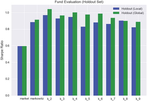
Sharpe Ratios result during the holdout period for each model are plotted and compared for both the local and global asset allocation approaches. All of the state-based portfolios showed ratios greater than that of the market, and several exhibited superior performance to Markowitz’s portfolio. More specifically, the two-state portfolios yielded the highest Sharpe Ratios for both local and global optimizations followed by the four-state variant. See Figure 2. The global optimization method out-performed the local method in all versions except the eight-state model in which the rations were comparable.

Figure 2. Performance of portfolios created using models with states k = 1 (Markowitz) to k = 9

Table 1: Portfolio allocations in a 2 and 4 state examples for Local and Global optimization approaches.

Table 1. Summarizes the asset allocation decisions made for the two and four-state portfolios. Results for both the Local and Global optimization approaches are included

	Two State				Four State
	Local		Global		Local				Global
Asset	0	1	0	1	0	1	2	3	0	1	2	3
EFA	0.07				0.03		0.03
EEM	0.02				0.08		0.01
AGG	0.68	1.00	0.76	1.00	0.74	1.00	0.64	1.00	0.49	1.00	1.00	1.00
RUT
IXIC	0.22		0.24		0.12		0.32		0.51
GSPC					0.04
Total Allo cation	1.00	1.00	1.00	1.00	1.00	1.00	1.00	1.00	1.00	1.00	1.00	1.00

By looking at the asset allocation in the two-state model, State 0 is a bullish period associated with advancing market prices. This can be seen in the local variant with allocations to international equity markets (EFA, EEM) and to domestic technology (IXIC, a.k.a NASDAQ Composite) in addition to the aggregate bond index (AGG).

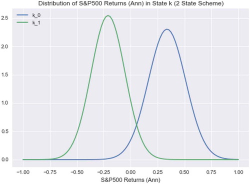
Similarly, the portfolio derived through global optimization is bullish but takes equity exposure through technology (IXIC) instead of emerging market equities as the local portfolio does. Conversely, State 0 is exclusively allocated to the bond fund, which is the most conservative and least-volatile asset in the universe of potential investment options making it the best option in periods of broad-based market declines. The global allocation identified State 0 as a bearish state associated with market declines and invested exclusively in bonds as well. The deductions about the nature of the states made by examining the asset allocations of the model portfolios are supported by description graphs shown in Figure 3. The figure shows that the market baseline (S&P 500) exhibited positive growth during periods in State 0 as compared to periods in State 1 when it experienced negative returns. This supports the allocation results from Table 1.

Figure 3. Generalized performance of States 0 and 1 from two-state model. Assumption of normality solely for purposes of illustration based on mean and standard deviation

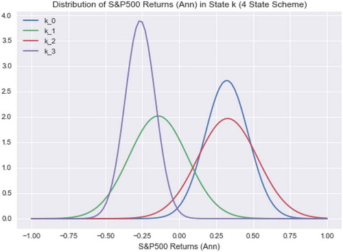
The four-state model also offered superior Sharpe Ratio performance to both market and the single-state Markowitz portfolio. The Local optimization variant allocated exclusively to bonds (AGG) for States 1 and 3 while making allocations to equities when in States 0 and 2 as shown in Table 1. This decision is consistent with the information in Figure 4, which shows that the S&P 500 experienced negative performance in the States 1 and 3. States 0 and 2 exhibited positive baseline performance supporting the case for assuming risk during such periods.

The Global optimization results were also allocated solely to AGG when in States 1 and 3; however, it also allocated to bonds in State 2 differing from the allocation guidance from the Local optimization method. Examining Figure 4 it can be seen that while State 2 has a comparable positive-expected return it also has a larger standard deviation in return thereby increasing the uncertainty in outcomes. This uncertainty in expected returns for assets in this state impacted the asset allocation under the Global methodology. Since the two optimization methodologies employ different objective functions, different allocation solutions are determined as optimal, which can be illustrated by the allocation to the conservative bond asset in State 2.

Figure 4. Generalized performance of States 0 and 1 from four-state model. Assumption of normality solely for purposes of illustration based on mean and standard deviation

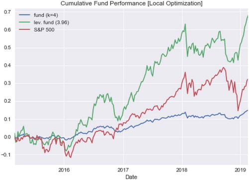
Figures 5 and Figures 6 illustrate the portfolio performance figures summarized in Figure 4. Portfolios generated by the two and four-state models have similar performance characteristics. Given that the objective of the optimization was to minimize the Sharpe Ratio, the resulting portfolios placed a premium on low-volatility allocation. Low-volatility performance came at the expense of higher returns. The tradeoff between risk and returns is illustrated in Figure 4. All of the state-based portfolios have higher Sharpe Ratios than the market but have lower annualized returns. In order to address the issue of underperformance relative to the market, the level of portfolio risk is increased through leverage using Equation (20)(20) $l=\frac{{\sigma }_{mkt}}{{\sigma }_{port}}$(20) . When this leverage factor is applied to portfolio performance, all state-based portfolios produce returns greater than the market while maintaining market-level risk. Additionally, both of the multi-state portfolios produced higher returns than the single-state Markowitz portfolio while also achieving a better risk-return profile with higher Sharpe Ratios. Table 2 summarizes the performance of each model variation.

Figure 5. Performance-leveraged and non-leveraged portfolio of Local, two-state model

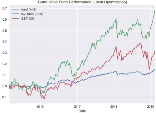
Figure 6. Performance-leveraged and non-leveraged portfolio of Local, four-state model

4.2. French-Fama considerations

The performance of the state-based portfolios was investigated further using the principles from the seminal factor⁶ investing research conducted by French and Fama (1992). The French-Fama model is designed to describe portfolio returns using three factors: (1) market risk, (2) outperformance of small companies compared to big ones (SMB), and (3) outperformance of high book value companies relative to low book value companies.

(22) $r_{port}=R_f+\beta \ast Mkt+{\beta }_s\ast SMB+{\beta }_v\ast HML+\alpha$(22)

Analyzing portfolio returns using Equation (22)(22) $r_{port}=R_f+\beta \ast Mkt+{\beta }_s\ast SMB+{\beta }_v\ast HML+\alpha$(22) identifies that the two factors – market returns and HML (high value versus low)—were significant factors as indicated in Table 3. Market performance and the discrepancy in the performance of high and low-value companies were the most influential factors in the performance of the two-state local model portfolio. Company size as captured by the SMB feature did not influence returns as much as the other two factors as indicated by the p-value of 0.430 and was not considered statistically significant. The French-Fama model had an F-statistic of 56.01 and $R^2$ value of 0.45, which only explained 45% of the variability in returns. By comparison, French and Fama published that the three-factor model explained more than 90% of the returns for a well-diversified portfolio (Fama & French, 1992). The discrepancies between model $R^2$ values indicate that the state model is considering factors not captured by the French-Fama factors.

Table 2. Summary of portfolio performance attributes during the holdout period

		Sharpe	Annualized		Ann. Lev.
Portfolio		Ratio	Return	Leverage	Return
Market		0.593	0.085	—	—
Markowitz (k = 1)
	Global	0.913	0.029	4.473	0.136
	Local	0.883	0.029	4.265	0.126
Two-States (k = 2)
	Global	1.042	0.034	4.383	0.155
	Local	0.968	0.035	3.963	0.141
Four-States (k = 4)
	Global	1.002	0.034	4.394	0.151
	Local	0.946	0.035	3.960	0.139

Table 3. Summary of Linear Model to Predicting Portfolio Results using French-Fama Factors

Feature	Coefficient	Std. Error	p-value
Intercept	0.0002103	0.0002661	0.430
Mkt	0.0015103	0.0001455	2e-16
SMB	−0.0003004	0.0002382	0.209
HML	−0.0015440	0.0002175	2.11e-11

5. Conclusions & future work

This article presents a new approach for designing investment portfolios using a discrete state-based framework for classifying periods of time in the financial markets. State membership decisions are made using unsupervised machine learning algorithms, which make assignments based on a two-dimensional feature set consisting of expected growth and covariance values. States are created by grouping observations with similar features.

The article goes on to introduce two new approaches for designing portfolios through optimization using the underlying analytical framework of transitional dynamics of discrete states. After defining states and designing state-specific portfolios using data from a training period, the models were applied to a separate holdout dataset for testing. The results showed that the multi-state portfolios created using this method produced higher Sharpe Ratios than both market and single-state Markowitz portfolios. It also demonstrated that applying leverage to the portfolios resulted in returns superior to the market and Markowitz while only assuming only market-level risk.

The portfolio performance observed as part of this research demonstrated the promise of this innovative new approach to portfolio design and the need for future research in this domain. Traditional investment management strives to outperform the S&P 500 and the critically acclaimed work of Markowitz established the first systemic approach to portfolio design. This research demonstrated that a state-based approach can produce portfolios that are capable of outperforming market and Markowitz portfolios on a risk-adjusted basis.

State-based techniques, such as this one, are not without shortcomings. Specifically, the state definitions are sensitive to the training periods on which the states are built. If the training period does not observe market behavior similar to that in the testing period then it cannot adequately respond to such conditions. For this reason, it is imperative that a robust training period be used in the state definition phase. This approach can be sensitive to the changes in asset performance relative to the markets. Further to the sensitivity to asset selection, consideration should be given to imposing constraints on the percentage of assets that can be allocated to an asset.

This research effort demonstrated the potential of applying a state-based methodology to portfolio design; however, a great deal of research in this space remains. Future research could build on the foundation of work presented in this article in several areas. First, perform an extensive study into the selection criteria of the number of states, $k$. This research has focussed on Sharpe Ratio and returns, but what other factors could offer value in the evaluation of portfolio performance. Further consideration should be made into the tradeoff between portfolio efficacy measures. Second, conduct a study into an expanded feature set. Inspiration was taken from the underlying parameters of MPT in this research – expected growth and covariance—and used to define states. Potential features for examination include technical market indicators, such as moving averages, relative strength index (RSI), and sentiment; economic indicators, such as OECD leading indicators; and interest rate information, such as yield curves. Lastly, research other methods for creating portfolios for each state. This research applied optimization in an effort to maximize the Sharpe Ratio of a portfolio. Additional research should examine whether the portfolios would benefit from using other objective functions to determine asset allocations.

Additional information

Funding

The authors received no direct funding for this research.

Notes on contributors

Matthew W. Burkett

Matthew Burkett, Ph.D., is a Senior Director at Ankura Consulting and was a member of the Financial Decision Engineering (FDE) research group while completing his Ph.D. at the University of Virginia where he collaborated with William T. Scherer, Ph.D., on research efforts ranging from agent-based simulations of financial markets, market microstructure, and portfolio decision theory and design.

William T. Scherer, Ph.D., is a professor of Systems Engineering in the School of Engineering and Applied Science, Associate Chair, and Director of the Accelerated Master’s Program (Systems Engineering) at the University of Virginia.

Notes

1. The adjusted closing price, denoted in Yahoo! Finance as “Adjusted Close” accounts for splits and dividends. Data is adjusted using dividend and split multipliers to reflect the total return of security, adhering to standards set by Center for Research in Security Prices (CRSP).

2. The macro signal set includes the following assets: US equity indices (S&P 500, NASDAQ, Russell 2000), US bond index (AGG—iShares Aggregate Bond), and international ETFs (EEM—iShares MSCI Emerging Markets, EFA—iShares MSCI EAFE).

3. The number of periods per level of data granularity is as follows. Note that the number of daily periods is an estimate of the number of annual trading days. Daily: 252, Weekly: 52, Monthly: 12.

4. The portfolio return variable $r$ is a generic representation denoting either $r_{local}$ from Equation (15)(15) $r_{local}=p_0^{(k)}{\mathrm{\Pi }}^n{W}_{local}^{\ast }R$(15) or $r_{global}$ from Equation (16)(16) $r_{glob}=p_0^{(k)}{\mathrm{\Pi }}^n{W}_{global}^{\ast }R$(16)

5. The “market”, as referenced in this article, is represented by the S&P 500 Total Return index.

6. Source for factor data used in comparison is Eugene French Data Library(Kenneth r. french data library, 2019)

References

- Ang, A., & Bekaert, G. (2002). International asset allocation with regime shifts. The Review of Financial Studies, 15(4), 1137–17. https://doi.org/10.1093/rfs/15.4.1137
- Burkett, M., Scherer, W., & Adams, S. (2020). The state of state in finance: A selective survey of discrete state applications in finance from Markowitz to machine learning.
- Burkett, M. W., Scherer, W. T., & Todd, A. (2019). Are financial market states recurrent and persistent? Cogent Economics & Finance, 7(just–accepted), 1622171. https://doi.org/10.1080/23322039.2019.1622171
- Dean, A., Voss, D., and Draguljić, D. (1999). Design and analysis of experiments (Vol. 1). Springer.
- Fama, E. F., & French, K. R. (1992). The cross-section of expected stock returns. The Journal of Finance, 47(2), 427–465. https://doi.org/10.1111/j.1540-6261.1992.tb04398.x
- Gkillas, K., Tsagkanos, A., & Vortelinos, D. I. (2019). Integration and risk contagion in financial crises: Evidence from international stock markets. Journal of Business Research, 104, 350–365. https://doi.org/10.1016/j.jbusres.2019.07.031
- Guidolin, M., & Timmermann, A. (2007). Asset allocation under multivariate regime switching. Journal of Economic Dynamics & Control, 31(11), 3503–3544. https://doi.org/10.1016/j.jedc.2006.12.004
- Hamilton, J. D. (1989, March). A new approach to the economic analysis of nonstationary time series and the business cycle. Econometrica, 57(2), 357. https://doi.org/10.2307/1912559
- French, Kenneth R. Data Library. french data library. (2019). https://mba.tuck.dartmouth.edu/pages/faculty/ken.french/data_library.html
- Luenberger, D. G. (1997). Investment science. OUP Catalogue.
- Lunde, A., & Timmermann, A. (2004). Duration dependence in stock prices: An analysis of bull and bear markets. Journal of Business and Economic Statistics, 22(3), 253–273. https://doi.org/10.1198/073500104000000136
- Markowitz, H. (1952). Portfolio selection. The Journal of Finance, 7(1), 77–91.
- (yahoo! help) what is the adjusted close? https://help.yahoo.com/kb/SLN28256.html