Customer comfort limit utilisation: Management tool informing credit limit-setting strategy decisions to improve profitability

Abstract

The key criteria for making business decisions is profit, so when making credit limit-setting strategy decisions, profitability will be the most important driver. The profitability of a credit limit-setting strategy is dependent on the customer’s utilisation of the limits set by the strategy. This points towards a need to determine the extent to which a limit can be increased before a customer’s utilisation will decline beyond the point of being profitable. This paper sets out to define a Customer Comfort Limit Utilisation (CCLU) measure that can be used to gauge a customer’s level of comfort (in terms of limit utilisation) with a newly proposed limit. The CCLU is defined as a function of the customer’s limit utilisation and credit limit; in simpler terms, it can be viewed as a function of balance growth vs limit growth. The neural network model that predicted utilisation first and then the CCLU based on the resulting utilisation values was selected as the final model. Once the final model was determined, it was then verified whether profitability could be improved by using a CCLU measure as a management tool when making limit-setting strategy decisions. It was found that strategies involving CCLU values could lead to increased profitability since CCLU values near 100 (i.e. the customer is 100% comfortable with the new limit and will utilise to the same extent as the previous one) are associated with higher key performance metrics levels.

Keywords:

• credit card limits
• prediction
• utilisation
• customer comfort
• profitability
• limit strategies
• management tool

PUBLIC INTEREST STATEMENT

Many banks use account-level profitability strategies regarding credit limit increases on credit cards. However, this only takes the bank’s profitability into account but not the customer’s comfort with the new limit. These two go hand in hand, seeing that the profitability of credit limit increases depends on credit utilisation rates, which is affected by the customer’s comfortability. Thus, there is a need to determine the extent to which credit limits can be increased before the customer becomes uncomfortable and his utilisation declines, and the limit increase becomes unprofitable for the bank. In this paper, a Customer Comfort Limit Utilisation (CCLU) measure is developed to measure a customer’s comfort level with new proposed limits. The CCLU is defined as a function of the customer’s limit utilisation and credit limit; in simpler terms, it can be viewed as a function of balance growth vs limit growth.

1. Introduction

Profitability drives business decisions, so when making credit limit strategies decisions, profitability will be the main driver. The profitability of credit limit increases, however, is largely dependent on the utilisation of the new credit limits. The reason is that when a customer receives a credit limit increase and the utilisation grows in line with the limit—i.e. the overall balance growth is the same or higher than the limit growth—the net interest income (NII) earned on the credit provided will increase. On the other hand, if the utilisation does not grow in line with the limit, the profit will be driven down because the amount of risk capital required to make provision for losses increases as limits increases. In addition, if the customer does not utilise the newly available credit limit in line with this increase in risk capital required, the return on regulatory capital (RORC) is negatively impacted.

This points towards a need to determine to what level a limit can be increased before a customer’s utilisation will decline beyond the point of being profitable. This paper sets out to define a Customer Comfort Limit Utilisation (CCLU) measure that can be used as a management tool to gauge a customer’s level of comfort (in terms of limit utilisation) with a newly proposed limit when making limit-setting strategy decisions.

Section 2 introduces credit limit utilisation rates and credit cards, it also summarises the factors influencing credit limit utilisation rates and the methods available to predict these. Section 3 describes the methodology applied to define the CCLU measure. In Section 4 the CCLU measure is applied to real credit card data and it was illustrated how it can be used as a management tool to make limit-setting strategy decisions. Section 5 concludes and provides some suggestions for future research.

2. Literature study

The literature study provides some general insights regarding credit limit utilisation rates and the prediction thereof since the CCLU measure aims to predict a customer’s level of comfort (in terms of credit limit utilisation) with a newly proposed limit.

2.1. Credit limit utilisation rates

Fulford and Schuh (2017) cited that utilisation rates indicate customers’ behaviour concerning credit limits. A utilisation rate is defined as the outstanding balance divided by the credit limit and could be used to measure the proportion of the limit used by the customer (Wait, 2021). One reason why one may be interested in utilisation rates is that the more a customer utilises the credit limit available, the more profitable the product becomes (Budd & Taylor, 2015). Thus a product’s profitability can be improved by taking the customer’s credit limit utilisation or, more specifically for this paper, taking the customer’s comfort with their limits into account when making credit limit-setting strategy decisions.

It is also important to note that according to Osipenko and Crook (2015) the utilisation of credit limits matures around six months after opening an account or after a credit limit increase.

2.2. Credit cards

Credit cards are unsecured lending products (Baesens et al., 2016) with the dual functions of acting as loans and as payment tools (Bellotti & Crook, 2009). These products are more complex than standard loans since their balances fluctuate and are largely dependent on customer behaviour (Huang & Thomas, 2014). Credit cards are offered to customers who qualify according to rules dictated by regulations, risk measurements and profitability (Thomas, 2009). Risk measurements include: probability of attrition, affordability of credit, probability of default and loss given default. Regulations require that banks maintain capital reserves (regulatory capital) as a percentage of the limit made available to a customer, as well as the balance spent using the risk-weighted assets (BCBS (Basel Committee on Banking Supervision), 2006). These two limitations, the complexity of the product and the regulations by which it is governed, emphasise the need for a CCLU measure that could be used to inform limit-setting strategy decisions to make this product as profitable as possible within the confines brought forward by these limitations.

The profitability of the product can be measured by key performance metrics (KPMs), such as NII and RORC. NII is defined as interest income (the interest the customer pays the bank on a negative balance on their credit card) less interest expense (the interest the bank pays the customer on a positive balance on their credit card). RORC is termed as the return made on regulatory capital, with regulatory capital being the amount of capital reserves the bank is required to hold against their assets as required by regulations (BCBS (Basel Committee on Banking Supervision), 2006). These two measures were used as KPMs for this paper since an increase in any of these will lead to an increase in profitability. To express both measures in terms of interest, the interest return on regulatory capital (IRORC) was used instead of RORC. The IRORC was calculated by dividing the total interest income by the regulatory capital.

2.3. Factors that influence credit card utilisation rates

This section provides a summary of the factors affecting credit card utilisation rates.

Kim and DeVaney (2001) proposed that the drivers of credit card payment behaviour are influenced by the following factors: consumption needs, current and future resources, consumer preferences as well as interest rate. The findings of Osipenko and Crook (2015) on the factors and characteristics influencing utilisation rates were similar. They used the following information in their study: behavioural characteristics (transaction data), application characteristics (time-fixed elements such as age, gender, marital status and occupation) and macro-economic characteristics (GDP, interest rate and unemployment rate).

Each of these factors as well as examples of the characteristics underpinning them are discussed in Appendix A. What follows is a brief investigation into the various techniques available to predict utilisation rates.

2.4. Methods available to predict utilisation rates

There are several different methods available to predict credit utilisation rates. Osipenko and Crook (2015) conducted a study on forecasting utilisation rates and used the following techniques: ordinary linear regression, fractional regression, beta regression and weighted logistic regression. Alternative methods also mentioned in the literature include ordinary logistic regression and machine learning techniques (e.g., neural networks). It should be noted that some of these methods were originally intended to predict recovery rates and loss given default (LGD) rates but since Osipenko and Crook (2015) explain that utilisation rates have the same distributional shape as recovery rates, all of these techniques could be used to model utilisation rates too.

These six different methods were investigated to find the most appropriate methods to predict utilisation rates for this paper. Three of these six methods were applied in the paper as these are the more commonly used techniques in literature and they were sufficient to address the objectives of the paper. The focus was not on the development of a superior model but on the demonstration of the proposed CCLU methodology. The three methods used are discussed below, while the discussion on the other techniques can be found in Appendix B.

2.4.1. Ordinary linear regression

Ordinary linear regression assumes that a linear relationship exists between the utilisation rate and the input variables. This is a relatively simple method but has the limitations that the statistical assumptions are not necessarily adhered to in every study. Furthermore, the assumed linear relationship may not account for more complex underlying relationships. Lastly, linear regression modelling results are unbounded outcomes and utilisation rates are bounded between 0 and 1, making it necessary to also use a conditional function (Osipenko & Crook, 2015).

2.4.2. Weighted logistic regression

Weighted logistic regression is an adaptation of ordinary logistic regression. The problem encountered with the ordinary logistic regression function, however, is that the output is binary (0 or 1). This is accompanied with a probability of a case being either 0 or 1. In this case, where the utilisation rate is a continuous variable, it means that it needs to be transformed into a binary variable. Osipenko and Crook (2015) suggested that the utilisation rate can be expressed as the probability of the limit being utilised or not. This approach creates two cases, where 0 indicates no utilisation and 1 indicates full utilisation (a 60% utilisation rate can then be interpreted as a 60% probability of a limit being fully utilised). This approach was endorsed by Van Berkel and Siddiqi (2012), who used a similar method to model LGD rates, as well as by Breed et al. (2019).

2.4.3. Machine learning technique

Machine learning techniques are alternative methods that could be considered when dealing with non-linear variables. Machine learning, however, is not a specific technique but rather computer algorithms that improve automatically through experience. Although these techniques provide better predictive power they are unfortunately also considered to be very complex (Wielenga et al., 1999).

One example of these algorithms is neural networks. Neural networks are often regarded as mysterious and powerful predictive tools, but on closer inspection, the most typical form of a neural network is simply a regression model with a flexible addition (Wielenga et al., 1999). This addition enables the neural network to model virtually any relationship between the input variables and the target variable (Breed & Verster, 2017). Some of the disadvantages of neural networks are the loss of interpretability and the loss of transparency of the model results due to the model complexity (Wielenga et al., 1999).

2.5. Literature summary

A utilisation rate is defined as the outstanding balance divided by the credit limit and could be used to measure the proportion of the limit used by the customer. Utilisation rates normally mature around six months after opening an account or after a credit limit increase. It is thus suggested that a time frame of six months be used when predicting utilisation rates.

The complexity of credit cards (the fluctuating balances and the dependency on customer behaviour) as well as the regulations the product are governed by emphasising the need for a CCLU measure that could be used to inform limit-setting strategy decisions to increase profitability. The profitability of the product can be measured by some KPM, such as NII and RORC.

The evaluation of the factors influencing credit card utilisation rates found that these factors can be summarised as: consumption needs and application characteristics, current and future resources, consumer preferences and behavioural characteristics, as well as socio and macro-economic factors. It is recommended that characteristics describing all of these factors should be included when modelling credit card utilisation rates. However, macro-economic factors were excluded from this paper since account level modelling was used and macro-economic factors affect the whole population rather than just a few selected individuals.

Various methods to predict utilisation rates, which turned out to be different variations of linear and logistic regression, were investigated. The study by Osipenko and Crook (2015) found that ordinary linear regression and fractional regression performed the best when comparing the predictive power and shape of the distributions. The other methods, however, did not perform so differently either. It is recommended that machine learning techniques should only be considered where the explanatory variables have a non-linear relationship with the target variable. Based on not only this information and recommendations but also on the need for some variety in terms of the methods explored, the following methods will be deployed to predict credit limit utilisation rates for this paper: ordinary linear regression, weighted linear regression and neural networks.

The next section discusses the methodology; i.e. it explains how the information reflected in the literature study, especially the factors and characteristics influencing credit card utilisation rates and the methods that could be used to predict the utilisation rates, was utilised to ultimately predict CCLU values.

3. Methodology

According to industry research by Osipenko and Crook (2015), the utilisation of a credit limit matures around six months after the account has been opened or a credit limit has increased. This indicates that a customer tends to return to a certain level of credit utilisation six months after a credit limit increase. This level of utilisation points towards customers having a certain level of comfort with the credit available to them.

If a customer receives a credit limit increase that they are comfortable with, the utilisation of the credit limit stays the same and the balance growth is proportionally in line with the limit growth, hence the profitability of the account will be favourably affected. This is due to, among other things, the increase in interest earned. However, should a customer receive a credit limit increase that they are not comfortable with and the utilisation of the new credit limit does not grow in line with the limit increase, the profitability of the account will be adversely affected.

One of the reasons for this is that the amount of risk capital required increases as limits increase, but if the customer does not utilise the new credit limit in line with this increase, the RORC is negatively impacted. Figure 1 illustrates the impact on utilisation rates if the balance growth after a credit limit increase is not in line with the limit growth. It is shown that even though the limit increased by R5 000 (from R20 000 to R25 000) the balance increased by only R2 000 (from R10000 to R12 000) resulting in a utilisation rate drop from 50% to 48%.

Figure 1. Top: The effect of a credit limit increase on utilisation rate (UT).

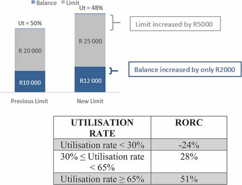
3.1. Bottom: Utilisation rates and RORC

The bottom part of Figure 1 (based on real data) further shows that the RORC will decrease as utilisation rates decrease. This illustrates that a limit can be increased to a point where the customer no longer feels comfortable with spending at their typical utilisation rate and that a limit can be increased to a point where it is no longer profitable.

3.2. Definition of the CCLU measure

Currently, no measure exists to determine a customer’s level of comfort. The suggested CCLU measure determines customers’ comfortability (in terms of utilisation) with new limits. This measure is defined by the following equation:

(1) $CCL{U}_i=\frac{balancegrowt{h}_i}{limitgrowt{h}_i}\times 100$(1)

where:

$CCL{U}_i$ is the Customer Comfort Limit Utilisation measure for customer $i$,

$balancegrowt{h}_i=\frac{balanc{e}_{1i}-balanc{e}_{0i}}{balanc{e}_{0i}},$

$limitgrowt{h}_i=\frac{limi{t}_{1i}-limi{t}_{0i}}{limi{t}_{0i}},$

$balanc{e}_{0i}$ and $balanc{e}_{1i}$ are the balances for customer $i$ before and after a credit limit increase (indicated by subscript 0 and 1 respectively), and

$limi{t}_{0i}$ and $limi{t}_{1i}$ are the limits for customer $i$ before and after a credit limit increase, (indicated by subscript 0 and 1 respectively).

It should be noted that once this measure has been defined, the CCLU measure can be predicted in two different ways: by predicting the new utilisation rate first and then deriving the CCLU measure based on that rate, or by predicting the CCLU measure directly. Under the first approach, the customer’s new credit utilisation rate is predicted ($utilisationrat{e}_{1i}$) and $balanc{e}_{1i}$ is then derived from this by using:

(2) $balanc{e}_{1i}=predictedutilisationrat{e}_{1i}\times limi{t}_{1i}$(2)

Once $balanc{e}_{1i}$ has been derived, all the information can be plugged into equation (1)(1) $CCL{U}_i=\frac{balancegrowt{h}_i}{limitgrowt{h}_i}\times 100$(1) and the predicted CCLU measure can be calculated. Note that equation (2)(2) $balanc{e}_{1i}=predictedutilisationrat{e}_{1i}\times limi{t}_{1i}$(2) comes from the definition of utilisation rates, namely $utilisationrat{e}_{1i}=\frac{balanc{e}_{1i}}{limi{t}_{1i}}$ (and $limi{t}_{1i}$ will be known as this is the new limit).

Although customers’ risk grades are not explicitly taken into account by this definition, they will inherently be taken into account since the limit increases offered to a customer are based on the customer’s risk grade. Only customers who qualified for a limit increase in terms of regulatory requirements, bank policies including discretion, affordability and risk checks would be offered limit increases and thus are dealt with in this paper.

Concerning the interpretation of the CCLU measure: lower index values signify lower comfortability and higher index values signify higher comfortability. A resulting CCLU value of 100 intuitively translates to a customer being 100% comfortable with the new limit, meaning that they would utilise the new limit to the same extent as the previous one. Conversely, a CCLU value of 80 translates to a customer being only 80% as comfortable with the new limit as they were with the previous limit, indicating that the customer will utilise the new limit to a lesser extent than the old limit.

For an illustrative example refer to Table 1, which is an expansion of the example provided in Figure 1. In the example, a customer’s balance was R10 000 before a limit increase and the limit itself was R20 000, thus the limit utilisation was 50%. Once the customer’s limit was increased, the new balance is R12 000 and the new limit is R12 000, thus the new utilisation rate is 48%. The customer is therefore using the new limit to a slightly lesser extent (50% vs 48%) so the customer is 80% as comfortable with the new limit as they were with the old limit—the CCLU = 80.

Table 1. Illustration of the interpretation of the CCLU measure

Old balance	R10 000	New balance	R12 000
Old limit	R20 000	New limit	R25 000
Old limit utilisation	50%	New limit utilisation	48%
Balance growth = (R12 000-R10 000)/R10 000 = 20%
Limit growth = (R25 000- R20 000)/R20 000 = 25%
CCLU = balance growth/limit growth = 80
CCLU % = balance growth/limit growth = 80%

To make limit increase strategy decisions that would improve profitability, a customer’s expected comfortability needs to be determined before making a limit increase. Note that although the CCLU predicts a customer’s comfortability with a new limit six months or more (6+) after the limit increase, the predicted value is required before the credit limit increase takes place. More specifically, it is needed when the strategy decision regarding the limit increase is made.

Now that the CCLU measure had been defined important questions that also need to be answered are whether or not models can be developed to predict these CCLU values before making limit-setting strategy decisions, and whether the predicted CCLU values can be used to inform limit increase strategies to improve profitability. The methodology followed to develop models to predict CCLU values and illustrate the effect of using CCLU-based limit-setting strategies on profitability is discussed next, starting with the data preparation required for the models. The data preparation and model development were performed using the SAS Institute Inc (2020) software.

3.3. Data preparation

The first stage of the modelling process was to retrieve and prepare the data for model input. The data used for this paper consisted of transactional data from a large South African bank’s retail credit card database, and bureau data describing customers’ behaviour on credit cards not granted by this bank (termed as “outside cards” from here onwards). Only in-order accounts (i.e. not in arrears) were used. Only accounts that had a limit increase at least six months before the date of extraction were used. The reason was that since one wants to predict a customer’s comfortability with a new limit and since it was shown that utilisation typically matures six months after a limit increase, the data used to predict the comfortability should also reflect information at least six months after the last limit increase. The final dataset consists of over 90,000 observations with 132 variables collected over 2 years.

Once the final dataset was obtained, the following data preparation steps were performed to ensure good modelling principles: variable transformation, handling missing values, scaling variables, data partitioning, clustering levels of categorical variables, binning levels of numerical (interval) variables, clustering correlated variables, and removing statistically irrelevant variables (SAS Institute, 2010). More detail can be found in Appendix C.

Although the original dataset consisted of over 100 variables, only 22 were left after the data preparation step (refer to Table C1 for a list of these variables). As recommended, these variables represented all the factors influencing credit card utilisation rates. The only factor not represented was the macro-economic factor seeing that changes in these types of variables will affect the whole population in the same manner. Once all the data preparation steps were complete, the modelling process followed.

3.4. Model development

Two different approaches were followed to develop models to predict CCLU values. The first approach develops a model to predict the new utilisation rate first and then the new balance is derived from this by using equation (2)(2) $balanc{e}_{1i}=predictedutilisationrat{e}_{1i}\times limi{t}_{1i}$(2) . Once the new balance has been derived, the predicted CCLU value can be calculated by plugging the information into the CCLU equation (1)(1) $CCL{U}_i=\frac{balancegrowt{h}_i}{limitgrowt{h}_i}\times 100$(1) . The second approach develops a model to predict the CCLU value directly. Three models were developed using the first approach and one using the second approach.

The three models used to predict utilisation rates were: ordinary linear regression (Model 1), weighted logistic regression (Model 2) and a neural network (Model 3). A neural network was also used to predict the CCLU values directly (Model 4). Each modelling technique was briefly reviewed in the literature study and a discussion of how it was applied in this paper follows below. Stepwise regression at a significance level of 0.005 was used to select the statistically significant variables. In the case of the neural networks, stepwise regression was used to determine the statistically significant variables before fitting the models.

Once the models were developed, the models were compared and the best performing model was chosen as the final model.

Model 1: Ordinary linear regression to predict utilisation rates

Ordinary linear regression was used to develop Model 1 using the first approach.

Model 2: Weighted logistic regression to predict utilisation rates

Weighted logistic regression was used for Model 2 that also predicts utilisation rates. As discussed in the literature study, this technique creates two cases where 0 indicates no utilisation and 1 indicates full utilisation, with the actual utilisation used as the weight variable.

Model 3: Neural network to predict utilisation rates

The neural network model that could be used to predict utilisation rates was developed by applying the default settings of the software being used; feed-forward with three hidden layers.

Model 4: Neural network to predict CCLU values

A feed-forward neural network with three hidden layers was also used to develop a neural network model for the second approach; i.e. to predict the CCLU values directly.

3.4.1. Model comparison and selection

The models were compared according to the model development approaches followed. Thus, the three models developed to predict utilisation rate were compared among one another and the best performing model was selected. Only one model was developed to predict CCLU values and therefore this model was automatically selected for this approach. Finally, these two chosen models (one for each approach) were compared in terms of the mean squared error (MSE) and root mean squared error (RMSE) based on the predicted vs actual CCLU values to select the final model.

3.5. Illustrating the effect of using CCLU-based limit-setting strategies on profitability

Once the final model had been selected, the effect of using the CCLU values to inform limit-setting strategies was determined. The KPMs used were NII and RORC (IRORC to express both measures in terms of interest).

The illustration of the effect of using CCLU-based limit-setting strategies starts with investigating the relationship between NII, utilisation rates and CCLU values by plotting the average NII against utilisation rates and CCLU values simultaneously. This was done to determine if it would be worthwhile to use CCLU values to inform limit-setting strategies.

Next, some analyses were performed to test the effect that using CCLU-based limit-setting strategies could have on the NII and IRORC, and thus, ultimately also on the profitability of the product. The expected percentage increase in NII and IRORC of four strategies, based on different scenarios of strategies informed by the CCLU values, were calculated and compared.

The results from applying the CCLU definition to real data, the models resulting from following the discussed methodology and a summary of the analyses to illustrate the effect of using CCLU values in limit-setting strategy decisions are provided in the next section.

4. Results

This section documents the results derived by applying the previously discussed methodology.

4.1. Applying the CCLU definition

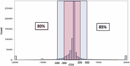
Figure 2 shows the distribution of CCLU values when equation (1)(1) $CCL{U}_i=\frac{balancegrowt{h}_i}{limitgrowt{h}_i}\times 100$(1) has been applied to the credit card data of a large South African bank. It reflects that the CCLU values ranged from—2 000 to 2 000. The two peaks at—2 000 and 2 000 reflects bucketed CCLU extreme values. Further analysis shows that 80% and 85% of the CCLU values fall within the −300 to 300 range (pink block) and—500 to 500 range (blue block), respectively, therefore this paper focuses on CCLU values within this range since it excludes data abnormalities. Some abnormalities resulted due to data errors, for example, if the limit or balance were incorrectly captured on the system as very small amounts (e.g., omitting the zeros at the end of a R value).

Figure 2. Distribution of CCLU values when the definition is applied to real data.

4.2. Model development

Three different models were developed to predict utilisation rates that, in turn, could be used to calculate predicted CCLU values. These models were developed using the following techniques: ordinary linear regression (Model 1), weighted logistic regression (Model 2) and a neural network (Model 3). Model 4 was also developed using a neural network, but this model was developed to predict the CCLU values itself. The variables selected for the four developed models differed somewhat. Table 2 compares the variables selected by the different models (only selected variables are displayed, thus only 15 of the possible 22 variables reflected in Table C1 are listed in Table 2). Eleven of the 15 selected variables were included in all the models.

Table 2. Variables selected for the different modelling techniques

	Utilisation rate models			CCLU model
	Model 1	Model 2	Model 3	Model 4
Variables	Ordinary linear regression	Weighted logistic regression	Neural network	Neural network
Average debit balance (scaled & binned)		X		X
Three-month average of fees on bank’s card due to transactions (binned)	X	X	X	X
Three-month average of the maximum utilisation of an outside card (binned)	X	X	X	X
Three-month average of the value of payment on the bank’s own cards before CLI (scaled & binned)	X	X	X	X
Three-month average of the value of the turnover on bank’s own cards before CLI (scaled & binned)	X	X	X	X
Three-month average of the volume of cash transactions on bank’s own cards before CLI (binned)	X	X	X	X
CLI amount (scaled & binned)	X	X	X	X
Current limit after CLI (scaled & binned)	X	X	X	X
Debit order type (e.g., full balance, minimum, fixed amount, etc.) (clustered)			X
Customer gender			X
Indicator of overall marketing consent	X	X	X	X
Month-on-book since customer joined the bank	X	X	X	X
Product group in which customer falls (clustered)	X	X	X	X
Three-month average of the total limit at outside cards before CLI (scaled)	X	X	X
Utilisation month-end before CLI	X	X	X	X

4.3. Model comparisons

The three utilisation models were compared among one another and the best performing model was selected based on the MSE and RMSE. The model developed to predict the CCLU values directly was automatically selected since only one such model was developed. Therefore, once the best performing utilisation rate model was identified, this model was compared to the CCLU value model to select the final model. Performance, in this case, was based on the MSE and RMSE for the predicted and actual CCLU values.

4.3.1. Utilisation rate models

Table 3 compares the MSEs and RMSEs of the three utilisation rates models on both training and validation data.

Table 3. Result comparison of utilisation rate models

MODEL	ORDINARY LINEAR REGRESSION (Model 1)		WEIGTED LOGISTIC REGRESSION (Model 2)		NEURAL NETWORK (Model3)
	MSE	RMSE	MSE	RMSE	MSE	RMSE
TRAIN	0.07	0.27	0.07	0.27	0.06	0.24
VALIDATION	0.08	0.29	0.17	0.41	0.05	0.23

The model with the lowest MSE for both the training and validation data is the neural network model. Initial investigations showed that the model’s performance is probability attributed to the presence of non-linearity in the data (one of the benefits of neural networks).

Another aspect that needs to be taken into account is the difference between the MSEs and RMSEs of as large differences in these indicates possible over-fitting. The weighted logistic regression model displayed a large difference between the fit-statistic of the training and validation data. The neural network model had the smallest difference when comparing the MSEs and RMSEs for the training and validation data, which indicates that possible over-fitting did not occur for this model.

Therefore, the neural network model (Model 3) was selected as the best performing utilisation rate model.

4.3.2. Best utilisation rate model vs CCLU model

Table 4 provides the MSEs and RMSEs of Model 3 (the best utilisation rate model) and Model 4 (CCLU model). These MSEs and RMSEs were based on the actual and predicted CCLU values. The predicted CCLU values of Model 3 have been derived based on the utilisation rates predicted by the model. The CCLU values of Model 4 have been predicted by the model itself.

Table 4. Result comparison of best utilisation rate model and CCLU value model

MODEL	CCLU values derived from NEURAL NETWORK UTILISATION RATE model (Model 3)		CCLU values predicted directly by NEURAL NETWORK (Model 4)
	MSE	RMSE	MSE	RMSE
TRAIN	157.56	12.55	340.86	18.46
VALIDATION	174.93	13.23	358.71	18.94

The MSE and RMSE for both the models are fairly large and indicate that neither models are very accurate, but it does indicate that predicting the CCLU values from the utilisation rate neural network model produces better results than predicting the CCLU values directly. For this reason, Model 3 of approach one was selected as the final model.

4.4. Performance of the final model

To investigate the performance of the final model, the actual utilisation rates (blue) were compared to the predicted utilisation rates (red) visually in Figure 3 (a) and (b). To further investigate the utilisation rate neural network model’s performance, the distribution of the actual CCLU values (blue) are also compared to the distribution of the predicted CCLU values (red). The actual utilisation rates are more condensed at high and low utilisation rates, whereas the predicted utilisation rates are more evenly distributed. The top-left graph reflects that the predicted CCLU values are slightly lower than the actual CCLU values since they are centred on lower CCLU values. The distribution shape of the predicted CCLU values, however, does still closely resemble the distribution of the actual CCLU values.

Figure 3. Comparison of actual and predicted utilisation rates in panels (a), (c), (d) and CCLU values in panels (b), (e) and (f).

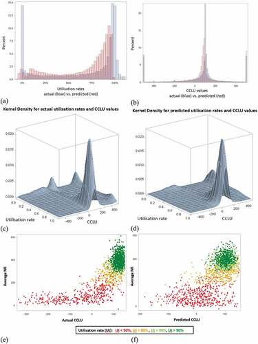
In Figure 3 (c) and (d), three-dimensional distributions of actual utilisation rates and CCLU values, as well as predicted utilisation rates and CCLU values, are used to further evaluate the final model. These plots show similar distribution shapes except for the predicted relationship lacking certain peaks in the distribution at lower utilisation rates. The natural interpretation of CCLU values is between 0 and 100 and from the Kernel Density graphs, it is clear that the bulk of the data fall within this range. Although the data anomalies have been excluded (due to the—500 and +500 limits) some data anomalies still exist in the data. An example of a data anomaly is if a customer deposits their bonus into their credit card, the utilisation will seem to be negative for some time thereafter. Data errors, for example, if the limit was incorrectly captured on the system as a R1 instead of R1 000, will result in abnormalities since the calculated utilisation will be exceptionally high.

The Figure 3 (e) and (f) which display the Average NII vs. Actual CCLU and Average NII vs. Predicted CCLU which confirm that higher utilisation rates are associated with higher NII. It also confirms that CCLU values near 100 are the most profitable.

These results confirmed that the best method to predict CCLU values is to first predict utilisation rates by using a neural network (Model 3) and then calculate the predicted CCLU values based on the utilisation rates obtained.

4.5. Illustration of the effect of using CCLU-based limit-setting strategies on profitability

To understand the impact of using a measure like this, the relationships between some of the product’s KPMs and utilisation rates, as well as the CCLU values need to be understood first, since the profitability can only be effective if there indeed are such relationships. Therefore, this section starts by exploring some of these relationships. Finally, the results of the analyses performed to illustrate the effect of using limit-setting strategies based on CCLU values are documented.

4.5.1. Relationship between NII, utilisation rates and CCLU values

One of the KPMs considered in the paper is NII, since changes here would also affect the profitability of the credit card product. Figure 3 (e) and (f) evaluates the relationship between average NII, utilisation rates and actual CCLU values simultaneously.

Figure 3 (e) and (f) confirms that higher utilisation rates are associated with higher NII. It also confirms that CCLU values near 100 lead to higher NII and are therefore more profitable. This proves that it would be worthwhile to use CCLU values to inform limit-setting strategies. Figure 3 (e) and (f) also portrays the average NII against the utilisation rates and actual CCLU values predicted by the final model. The same trend occurs but the predicted utilisation rates are more evenly spread and the predicted CCLU values are less condensed than the actual CCLU values.

4.5.2. Evaluation of the effect of using CCLU-based limit-setting strategies on profitability

Since it was proven that there is a relationship between the CCLU values and NNI, the next step was to illustrate the effect that using CCLU values to inform limit-setting strategies could have on profitability. It should be noted that although the predicted CCLU values will have to be used in practice, the actual CCLU values were used for this part of the paper since it is purely for illustrative purposes.

Four different strategies informed by the CCLU values were suggested. The suggested credit limit increase strategies based on CCLU values followed the following rationale: (1) Customers with lower comfortability regarding new limits should receive smaller credit limit increase amounts to increase their utilisation and overall IRORC; (2) Customers with higher comfortability regarding new limits should receive higher or lower credit limit increase amounts depending on their risk. For Strategy 1, for example, the lower CCLU values were to receive only 10% of the original credit limit increase amounts and higher CCLU values were to receive 210% of the original credit limit increase amounts. For Strategy 4 the same rationale was followed for the lower CCLU values but at 80% of the original credit limit increase amounts. However, it was also assumed that higher CCLU values would be associated with higher risk customers and therefore the credit limit increase amounts were lowered to 90% of the original credit limit increase amounts.

The new credit limit increase amounts were calculated and these were used as input into the final model to obtain the predicted utilisation rates (based on these new limits). Next, the different strategies were evaluated according to the effect on the NII, IRORC and the change in credit limit increase amounts. Table 5 shows the results for the original credit limit-setting strategy of allocating 100% of original credit limit increase amounts to all the CCLU groups and the other suggested strategies. The optimal credit limit increase strategy will be the one that increases the NII and IRORC while keeping the credit limit increase amounts stable or increased.

Table 5. Illustration of the effect of using CCLU values to inform limit-setting strategies

	Original strategy	Suggested strategy 1	Suggested strategy 2	Suggested strategy 3	Suggested strategy 4
CCLU ≤ 0	100%	10%	80%	85%	80%
0 < CCLU ≤ 50	100%	50%	90%	85%	90%
50 < CCLU ≤ 90	100%	90%	95%	95%	100%
90 < CCLU ≤ 100	100%	130%	100%	105%	105%
100 < CCLU < 150	100%	170%	95%	110%	110%
CCLU ≥- 150	100%	210%	90%	120%	115%
Capital: % increase		0,77%	0,19%	0,05%	0,09%
NII: % increase		0,90%	0,33%	0,07%	0,11%
IRORC: % Increase		0,030%	0,033%	0,018%	0,006%
CLI: % Increase		10,00%	−8,30%	0,00%	0,00%

For Strategies 1 and 4, the NII and IRORC will be positively affected but the total credit limit increase amounts will also increase. For Strategies 5 and 6, the NII and IRORC will also be positively affected but the total credit limit increase amounts will remain constant. Therefore, this proves that CCLU values can be used as a management tool to influence credit limit strategies to increase profitability.

5. Conclusion and future research

Only customers who qualified for a limit increase in terms of regulatory requirements and bank policies (discretion, affordability and risk checks) would be offered limit increases, therefore credit risk would be taken into account before making any limit increase offers and falls outside the scope of this paper. This makes profitability the key driver for business decisions in terms of credit limit increases. The profitability of a credit limit-setting strategy is dependent on the customer’s utilisation of the limits set by the strategy. This is why this paper defined a CCLU measure that could be used to determine the extent to which a limit can be increased before a customer becomes unprofitable due to low utilisation rates.

This was achieved by firstly compiling a literature review in terms of introductions into the credit limit utilisation rates and credit cards, a summary of the factors influencing credit limit utilisation rates and the methods available to predict it.

This was followed by the main contribution of this paper, the definition of the CCLU. Next came the application for the CCLU measure on the credit card data provided by a large retail bank of South Africa.

The next contribution was the development of models to predict CCLU values, which was achieved by following two different approaches. The first was to develop a model to predict the utilisation rates, and three of these models were developed. Under this approach, the predicted CCLU values were calculated based on the utilisation rates predicted by the best performing model. Under the second approach, an additional model was developed. This model directly predicted the CCLU values. The two models (one for each approach) were compared in terms of prediction accuracy and the final model was selected. The final model was the neural network model, predicting utilisation first and then deriving the predicted CCLU values based on that. This utilisation model consisted of 14 variables with the most significant variables identified as customers’ previous utilisation before a credit limit increase, whether customers have given overall marketing consent (is the bank allowed to send the customer marketing material), the customers’ product group (type of credit card, e.g., Gold, Silver) and customers’ gender (literature suggests that females have more credit cards open). The utilisation model achieved a mean squared error of 5.3% on the validation datasets.

This was followed by an illustration to verify whether or not using a CCLU measure as a management tool when making limit-setting strategy decisions could improve profitability. It was found that strategies involving CCLU values could lead to increased profitability since CCLU values near a 100 (i.e. the customer is 100% comfortable with the new limit and will utilise to the same extent as the previous one) is associated with higher KPMs like NII and IRORC.

Although the currently defined measure could be used as a management tool to improve profitability, ideas for future research include additional factors to the modelling process such as macro-economic factors, explicitly including the risk grades of customers and customer affordability measures.

Disclosure statement

No potential conflict of interest was reported by the author(s).

Additional information

Funding

This work is based on research supported in part by the Department of Science and Innovation (DSI) of South Africa. The grant holder acknowledges that opinions, findings and conclusions or recommendations expressed in any publication generated by DSI-supported research are those of the author(s) and that the DSI accepts no liability whatsoever in this regard;Department of Science and Innovation, South Africa.

Notes on contributors

Tanja Verster

This research was conducted by the Centre for Business Mathematics and Informatics (BMI) at the North-West University (NWU). BMI is a leading tertiary risk training and research group for the financial services industry. It is actively involved in applied research projects conducted at several major financial institutions in South Africa. The research reported on in this paper initially formed part of such a financial services industry research project focussing on limit setting strategies, profitability and customers comfort. Karmi Visser completed her Master’s degree in BMI and is an employee at a retail bank in South Africa. Gerbus Swart, Joggie Pretorius and Lin-Marie Esterhuyzen are employees at retail banks in South Africa. Tanja Verster completed her PhD in Risk Analysis in 2007, and her research focuses on predictive modelling in the financial environment. Erika Fourie completed her PhD in BMI and lectures at the School of Mathematical and Statistical Sciences, NWU.

Appendix A:

Details of factors influencing credit card utilisation rates

Appendix A discusses the factors influencing credit card utilisation, these are tabled in Table A1.

Consumption needs and application characteristics

According to Kim and DeVaney (2001), the consumption needs of individuals and their households influence their use of credit limits. Consumption needs are different for each individual due to the difference in life stages. For example, an individual responsible for a household with dependents would have a greater consumption need than a single individual.

One of the most informative characteristics of consumption needs is age because it is an important indicator of a person’s current life stage. Findings demonstrate an inverse relationship between age and consumption, whereby younger individuals are more likely to utilise credit cards to meet their consumption needs than older individuals since older individuals will have more stable incomes to cover their needs.

Marital status is another important characteristic that influences consumption needs. Individuals who are married are more likely to have higher expenditures and thus a greater need for credit and credit cards than individuals who are not. This is especially so since marital status is positively linked to the number of dependents per individual as well as household size and consumption needs, and will increase with an increase in any of these two.

Current and future resources

Bryant (1990) described credit as a mechanism of transferring future resources to the present to increase current consumption. Hanna et al. (1995) found that economical resources like income, liquid assets, investment assets and real assets influence the utilisation of credit cards since individuals make credit usage decisions based on their current resources and their expected future resources. Individuals with restricted current resources but with the expectation that future resources will cover their costs are more likely to utilise their available credit. On the other hand, individuals with enough current resources are less likely to have high credit card utilisation rates.

Other characteristics that also influence credit usage from a resource perspective are the total amount of debt and the number of credit cards available to individuals. Individuals with more credit available to them tend to use the resource if other current resources are limited.

A customer’s product holding is another good indicator of current and future resources. Individuals who are classified as “wealthy” based on their product holdings are less likely to use their available credit since current resources are not limited. “Young professionals”, on the other hand, tend to utilise their available credit due to limited resources and increasing expenses associated with entering the housing market and becoming financially independent.

Consumer preferences and behavioural characteristics

Consumers can be divided into two types of users when it comes to the utilisation of credit cards: revolvers and transactors (or convenience users). Revolvers are characterised by outstanding balances that revolve from one month to the next and are paid off by monthly instalments and are more likely to have high utilisation rates (Curphey, 2016).

Macro-economic factors

Higher interest rates create a degree of reluctance to utilise credit seeing that high interest rates demotivate individuals to revolve their credit as it increases the interest charged. Transactors are not as influenced by changes in interest rates given the nature of their credit card use.

Table A1. Summary of the factors (and examples of their underlying characterising) influencing credit card utilisation

Factor	Example of characteristics
Consumption needs and application characteristics	Age Marital status Number of dependents Household size Time at physical address Years at employer Occupation Highest level of education
Current and future resources	Income Liquid assets Investment assets Real assets Total amount of debt Number of credit cards Product holding
Consumer preferences and behavioural characteristics	User type (revolver or transactor)
Macro-economic factors	Interest rates GDP Unemployment rate

Appendix B:

Other modelling techniques investigated

The other modelling techniques investigated were:

Fractional regression

Papke and Wooldridge (1996) suggest fractional logistic regression to ensure that the outcome is bounded between 0 and 1(by taking the difference of the current log transformation of utility rate minus the previous period’)., a generalised linear mixed model is applied to estimate the regression coefficients.

Ordinary logistic regression

A method suggested by Somers (2009) involves ordinary logistic regression and allocating utilisation rates to either 0 or 1. In this case, a 0 indicates that the limit is unutilised and 1 This method poses problems as the predefined definition of utilised and unutilised is somewhat subjective and could also be manipulated. Another limitation of this method is that there will be a large number of indeterminate cases (not allocated to 0 or 1), meaning that the ordinary logistic regression procedure will be unable to classify a large number of new cases into a particular group.

Beta regression

Ferrari and Cribari-Neto (2004) proposed beta regression for LGD modelling which can be applied to utilisation rates modelling due to the similar density functions. The beta probability density function serves to model probabilities linked to limited outcome ranges such as 0 and 1, with the parameters chosen in such a manner that it matches the shape of the utilisation rate distribution. Ordinary logistic regression is applied to estimate the dependence between the beta function and the predictors, followed by applying inverse transformation of the cumulative probability function to obtain the utilisation rate. In an adjusted beta regression with ordinary least-squares version provided by Osipenko and Crook (2015), the target variable is transformed into the beta distribution. and ordinary least-squares or generalised linear mixed models are used to find the regression coefficients. Unfortunately, both these beta regression methods are difficult to describe intuitively

Appendix C:

Application of the data preparation steps to the final dataset

The following data preparation steps were applied to the data:

• The transactional variables used were summarised by calculating averages over the three months before the credit limit increase under investigation.

• An investigation into the missing values in the dataset revealed that these can be attributed to customers lacking a certain product or quality and it was decided to treat these as a separate level as suggested by Siddiqi (2006). Note that most variables were binned.

• Variables of large monetary values were scaled to take the scale differences into account. The variables were scaled according to the variables’ means (i.e. if a variable’s mean is 43,000, all the values within the variable was divided by 10,000).

• Based on the credit limit increase dates, the dataset was partitioned into a training dataset (60,000 observations) and a validation dataset (30,000 observations).

• Levels of categorical variables were clustered to avoid quasi-complete separation (when a level of the categorical input has a target event rate of 0% or 100%—in this case, one of the logits in logistic regression will be infinite (SAS Institute, 2010).

• Numerical (interval) variables were binned (grouped) into percentiles to make the variables more linear (Siddiqi, 2006). Anderson (2007) and Verster (2018) suggested binning to remove the effect of outliers and to effectively handle missing values by adding a separate level/bin for missing values.

• The reduction of variables based on redundancy amongst the inputs variables was dealt with by using variable clustering. This procedure group correlated inputs variables with one another (SAS Institute, 2010). One variable per group was chosen as the cluster representatives based on the underlying correlations or business importance.

• Irrelevant variables were identified by using both Hoeffding and Spearman’s correlations. Variables that have p-values above 0.5 associated with them were considered to be statistically irrelevant (SAS Institute, 2010). None of the variables selected met the criteria to be removed due to irrelevancy.

Once these steps were applied to the data 22 variables were available for model proposes, provided in Table C1.

Table C1. List of the 22 variables available for model purposes

Number of outside cards

Average debit balance (scaled & binned)

Three-month average of fees on bank’s card due to transactions (binned)

Three-month average of the maximum utilisation of an outside card (binned)

Three-month average of the minimum utilisation of an outside card (binned)

Three-month average of the value of payment on the bank’s own cards before CLI (scaled & binned)

Three-month average of the value of the turnover on bank’s own cards before CLI (scaled & binned)

Three-month average of the volume of cash transactions on bank’s own cards before CLI (binned)

Average volume of payments (binned)

CLI amount (scaled & binned)

Current limit after CLI (scaled & binned)

Customer segment (clustered)

Debit order type (e.g., full balance, minimum, fixed amount, etc.) (clustered)

Customer gender

Indicator of overall marketing consent

Indicator that the customer does not have an outside card

Month-on-book since customer joined the bank

Product group in which customer falls (clustered)

Indicator of customers exhibiting revolving behaviour

Indicator of a secondary card

Three-month average of the total limit at outside cards before CLI (scaled)

Utilisation month-end before CLI

References

- Anderson, R. (2007). The credit scoring toolkit: Theory and practice for retail credit risk management and decision automation. Oxford University Press.
- Baesens, B., Rosch, D., & Scheule, H. (2016). Credit risk analytics. SAS Institute, Wiley.
- BCBS (Basel Committee on Banking Supervision). (2006). Basel II: International convergence of capital measurement and capital standards: A revised framework. Bank for International Settlements.
- Bellotti, T., & Crook, J., 2009. Loss given default models for UK retail credit cards. https://www.researchgate.net/publication/215991287_Loss_Given_Default_models_for_UK_retail_credit_cards[Accessed 25 October 2021]
- Breed, D. G., & Verster, T. (2017). The benefits of segmentation: Evidence from a South African bank and other studies. South African Journal, 113(9–10), 1–21 http://dx.doi.org/10.17159/sajs.2017/20160345.
- Breed, D. G., Verster, T., Schutte, W. D., & Siddiqi, N. (2019). Developing an impairment loss given default model using weighted logistic reegression: Ilustrated on a secured retail bank portfolio. Risks, 7(123), 1–16. https://doi.org/10.3390/risks7040123
- Bryant, W. K., 1990. The economic organization of the household. Cambridge University Press: https://doi.org/10.1017/CBO9780511754395.
- Budd, J. K., & Taylor, P. G. (2015). Calculating optimal limits for transacting credit card customers. The Journal of the Operational Research Society Papers 1506.05376, arXiv.org, Revised Aug 2015 doi:10.48550/arxiv.1506.05376 https://arxiv.org/abs/1506.05376
- Curphey, M., 2016. Credit card news [homepage on the internet]. http://uk.creditcards.com/credit-card-news/transactor-or-revolver-1375.php [Accessed 10 August 2018]
- Ferrari, S. L. P., & Cribari-Neto, F. (2004). Beta regression for modelling rates and proportions. Journal of Applied Statistics, 31(7), 799–815. https://doi.org/10.1080/0266476042000214501
- Fulford, S., & Schuh, S. (2017). Credit card utilization and consumption over the life cycle and business cycle (Working paper 17-14). Consumer Payments research centre, Federal Reserve Bank of Boston.
- Hanna, S., Fan, X. J., & Chang, Y. (1995). Optimal life cycle savings. Financial Counseling and Planning, 6, 1–15 https://content.csbs.utah.edu/~fan/research/04-1995HannaFanChangFCP.pdf.
- Huang, B., & Thomas, L. C. (2014). Credit card pricing and the impact of adverse selection. The Journal of the Operational Research Society, 65(8), 1193–120. https://doi.org/10.1057/jors.2012.173
- Institute, S. A. S. (2010). Predictive modelling using logistic regression.
- Kim, H., & DeVaney, S. (2001). The determinants of outstanding balances among credit card revolvers. Financial Counseling and Planning, 12(1), 67–79 http://citeseerx.ist.psu.edu/viewdoc/download?doi=10.1.1.587.8612&rep=rep1&type=pdf.
- Osipenko, D., & Crook, J. (2015). The comparative analysis of predictive models for credit limit utilization rate with SAS/STAT (Paper 3328-2015). SAS Global Forum.
- Papke, L. E., & Wooldridge, J. M. (1996). Econometric methods for fractional response variables with an application to 401(K) plan participation rates. Journal of Applied Econometrics, 11(6), 619–632. https://doi.org/10.1002/(SICI)1099-1255(199611)11:6<619::AID-JAE418>3.0.CO;2-1
- SAS Institute, 2020. The Official SAS site. www.sas.com[Accessed 15 February 2020]
- SAS Institute Inc. (2020). The SAS system for windows release 9.4 TS Level 1M3 X64_8PRO platform Copyright©.
- Siddiqi, N. (2006). credit risk scorecards: Developing and implementing intelligent credit scoring. John Wiley & Sons.
- Somers, M., 2009. Credit card initial limits: How much is too much? Edinburgh (Online), credit scoring and credit control conference XVII (Online) (The Business School of the University of Edinburgh).
- Thomas, L. C. (2009). Consumer credit models: Pricing, profit and portfolios. Oxford University Press.
- Van Berkel, A., & Siddiqi, N. (2012). Building loss given default scorecard using weight of evidence bins in SAS®Enterprise Miner™ (Paper 141-2012). SAS Global Forum.
- Verster, T. (2018). Autobin: A predictive approach towards automatic binning using data splitting. South African Statistical Journal, 52(2), 139–155 https://hdl.handle.net/10520/EJC-10ca0d9e8d.
- Wait, R., 2021. What is credit utilisation – And why does it matter? (Forbes website). https://www.forbes.com/uk/advisor/credit-cards/what-is-credit-utilisation-and-why-does-it-matter/ [Accessed 31 January 2022]
- Wielenga, D., Lucas, B., & Georges, J. (1999). Enterprise miner: Applying data mining. SAS Institute Inc.