An exchange rate model where the fundamentals follow a jump-diffusion process

Abstract

This paper presents some models of exchange rate with jumps, namely jump diffusion exchange rate models. Jump diffusion models are quite common in computational and theoretical finance. It is known that exchange rates sometimes exhibit jumps during some time periods. Therefore, it is important to take into account the presence of these jumps in exchange rate modeling in general. However, even the simplest jump diffusion model introduces some analytical difficulty in terms of finding a solution to the model. The models we analyze in this paper make use of Approximation Theory in order to come up with closed form solutions to the underlying variables. This approach leads to the branch of differential equations called functional differential equations and more specifically the so-called delay differential equations. Our approach leads to a second order delay differential equation. Though, in principle, these types of functional differential equations can be solved analytically in some cases, the task, in general, is quite enormous. We circumvent this technical difficulty by deriving an approximate solution using a power series expansion of the second order. Therefore, we derive a complete solution to the models and also investigate the model’s predictions of the exchange rate. We introduce two jump diffusion models. The first model examines the case where there are jumps with a constant magnitude. The second model considers the case of jumps of different sizes. These are relatively simpler cases to be analyzed. We will present some computational aspects in terms of the difficulty often encountered in estimating these types of models. The difficulty increases for the type of exchange rate models being considered in this paper. Taking advantage of the specification of the models we have estimated the parameters using a two-step M-estimation strategy that combines full information maximum likelihood estimation in the first step and the simulated method of moments in the second step.

Keywords:

• Exchange rates
• macroeconomic fundamentals
• jump-diffusion
• monetary model of exchange rate

JEL:

• F31
• G12

1. Introduction

Exchange rates data usually exhibit discontinuities. Barrow and Rosenfeld (1984), Ball and Torous (1985) provide evidence of the presence of jumps in daily stock returns. Nevertheless, these discontinuities are not apparent in many monthly and weekly data. Jorion (1988) examined this issue and provided evidence on the presence of jumps in the foreign exchange market, including stock markets. Cont & Tankov (2004) presented an extensive overview of tools that have been used in the literature to model financial time series, in particular stock and options data that exhibit jumps. If we maintain that exchange rate dynamics are similar to those of stock prices, as commonly argued and postulated, it is then a natural exercise to consider exchange rate models including jump processes and to investigate if observed exchange rate data are consistent with such models. A similar exercise was recently performed by Erdemlioglu, Laurent, and Neely (2015). Our paper is related to theirs in the sense that we are all trying to identify the best exchange rate model within a set of continuous time models. However, unlike Erdemlioglu et al. (2015) and several other authors (Akgiray & Booth, 1988; Bates, 1996; Ficura, 2015)1988, we will not introduce the jumps directly in the exchange rate process. We will rely on the monetary model of exchange rate determination which indicates that the exchange rate is primarily driven by the monetary fundamentals, namely the process $f(t)$. Given evidence of the presence of jumps in exchange rates, it follows naturally that these jumps must be captured in the fundamentals process. Several studies in the literature have documented the failure of the fundamentals to explain observed exchange rate movements (Cheung, Chinn, & Pascual, 2005; Meese & Rogoff, 1983). Using a more realistic process to model the macroeconomic fundamentals may lead to an exchange rate model that better fits the data. Therefore, in this paper, we will investigate an exchange rate model that adds a jump-diffusion component to the stochastic process governing the fundamental determinants of exchange rate, namely the process $f(t)$. The paper presents two models of jump-diffusion for the fundamentals. For each model, we provide approximate analytical solutions for the implied exchange rate process and discuss the estimation of the parameters.

2. Some preliminaries

As commonly done in the literature (Cont & Tankov, 2004) we introduce jumps in the fundamentals process using the Poisson process. In general, a jump-diffusion Stochastic Differential Equation (SDE) for the process $\{X(t)\}$ has the form

$dX\left(t\right)=f\left(X\left(t\right),t\right)dt+g\left(X\left(t\right),t\right)dW\left(t\right)+h\left(X\left(t\right),t\right)dN\left(t\right)$

$X(0)=x_0,$

where $\{W(t){\}}_{t\ge 0}$ is a standard Wiener process and $\{N(t){\}}_{t\ge 0}$ is a simple Poisson process with constant intensity $\lambda$. The two processes are assumed to be independent. The Brownian motion (BM) component provides the diffusion and the simple Poisson process provides the jump. Given that at this point we consider a simple Poisson process with time-independent intensity, then, the simple Poisson process $N(t)$ has a Poisson distribution with parameter $\lambda t$. In integral form, we have

$X(t)=X(0)+{\int }_0^{t}f(X(s),s)ds+{\int }_0^{t}g(X(s),s)dW(s)+{\int }_0^{t}h(X(s),s)dN(s).$

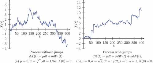
The first integral is a Wiener integral, the second one is an Ito stochastic integral (or possibly, a Stratonovich integral), and the last integral is a jump stochastic integral, where the stochastic process $\{h(X(t),t){\}}_{t\ge 0}$ is being integrated with respect to a simple Poisson process, a random measure. More generally, a jump stochastic integral could also be defined with respect to semimartingales or Levy processes. The fact is that whenever there is a jump process involved in either the SDE formulation or the stochastic integral formulation, the usual classical Ito’s lemma has to be modified to account for the jump or jumps. The following graphs (Figure 1) show examples of paths of the process $X(t)$ with and without jumps.

Figure 1. Paths of the process X(t) with and without jumps.

The use of Poisson processes to account for potential jumps makes the analysis simpler. Without any doubt, Poisson processes are one of the most important types of stochastic processes given their widespread use in modeling.

A basic example of the third integral is the following:

(1) ${\int }_0^{t}N(s)dN(s)=\frac{1}{2}\left(N^2(t)-N(t)\right).$(1)

As the solution indicates, this integral differs from the classical Riemann integral and also from the Ito integral with respect to a Brownian motion. More generally, it can be shown that

(2) ${\int }_0^t{N}^m(s)dN(s)=S_{N(t)-1}^{(m)},$(2)

where $S_n^{(m)}$ is the super-triangular numbers of order m for the first n positive integers, as defined by

(3) $S_n^{(m)}=\sum _{k=1}^n{k}^m$(3)

for non-negative integers m and n (Hanson, 2007).

At this point, we have a certain understanding of the three integrals defined in the jump-diffusion SDE as represented in the form of a stochastic integral equation. To solve the models presented in this paper, we need a version of Ito’s lemma (Ito, 1944) that accounts for jumps. The modified Ito’s lemma (Situ, 2005) is the following:

Consider the function $Y(t)=F(t,X(t))$, where $F$ is once continuously differentiable in t and twice continuously differentiable in $X$. Let the process $(X(t))t\ge 0$ satisfy the simple jump-diffusion SDE

(4) $dX(t)=f(t,X(t))dt+g(t,X(t))dW(t)+h(t,X(t))dN(t)$(4)

(5) $X(0)=x_0,$(5)

where the coefficient functions $f$, $g$, $h$, are possibly nonlinear in the state $X(t)$. Then

(6) $dF(t,X(t))=d_{(cont)}F(t,X(t))+d_{(jump)}F(t,X(t)),$(6)

where

(7) $d_{(cont)}F(t,X(t))=\left[F_t+F_{X}f+\frac{1}{2}{F}_{XX}{g}^2\right](t,X(t))+[F_X(t,X(t))g(t,X(t))]dW(t),$(7)

and similarly

(8) $d_{(jump)}F(t,X(t))=(F(t,X(t)+h(t,X(t))-F(t,X(t)))dN(t).$(8)

The function $F(t,X(t))$ referred to in this section will be derived from the monetary model of exchange rates.

3. Monetary model of exchange rate determination

The stochastic continuous time monetary model is set up as follows.

(9) $m(t)-p(t)=\varphi y(t)-\alpha i(t)$(9)

(10) $m^{\star }(t)-p^{\star }(t)=\varphi y^{\star }(t)-\alpha i^{\star }(t)$(10)

(11) $s(t)=p(t)-p^{\star }(t)$(11)

(12) $i(t)-i^{\star }(t)=\frac{{\mathbb{E}}_t[ds(t)]}{dt},$(12)

$m$, $p$, $y$, $i$, and $s$ are respectively money demand, the price level, output, the nominal interest rate, and the exchange rate and ${\mathbb{E}}_t()$ is the expectation conditional on information available up to time t. All the variables, except the nominal interest rate are in logarithm. Variables with a star superscript are foreign variables. The first equation (Equation 9(9) $m(t)-p(t)=\varphi y(t)-\alpha i(t)$(9) ) is the domestic money demand, the second (Equation 10(10) $m^{\star }(t)-p^{\star }(t)=\varphi y^{\star }(t)-\alpha i^{\star }(t)$(10) ) is the foreign money demand equation, the third equation (Equation 11(11) $s(t)=p(t)-p^{\star }(t)$(11) ) is the purchasing power parity, and the fourth equation (Equation 12(12) $i(t)-i^{\star }(t)=\frac{{\mathbb{E}}_t[ds(t)]}{dt},$(12) ) is the uncovered interest rate parity. The above four equations establish the following relationship between the exchange rate and the economic fundamentals $f(t)$:

(13) $\frac{1}{dt}{\mathbb{E}}_t[ds]-\frac{s(t)}{\alpha }=-\frac{f(t)}{\alpha },$(13)

where $f(t)$ is a function of real money balances and output defined as:

$f(t)=m(t)-m^{\star }(t)+\varphi (y(t)-y^{\star }(t)).$

In this paper, we follow Mark (1995) and set $\varphi =1$. The solution of the above stochastic differential equation provides the exchange rate as a function of the fundamentals

$s(t)=G[f(t)].$

Hence, the behavior of the fundamentals determine the behavior of the exchange rate. As a result, to solve the differential equation, the stochastic process that governs the fundamentals has to be specified. Moreover, if the exchange rate process exhibits jumps, such discontinuities are likely to originate from the fundamentals process. So, in this paper we model the behavior of the fundamentals using stochastic processes that account for jumps. In the following sections, we present two such jump-diffusion processes.

4. An arithmetic BM jump-diffusion process

According to the monetary model of exchange rate, sudden movements in exchange rates originate from abrupt movements in the fundamentals. In this section, we assume that at each point in time the fundamentals process exhibits a random number of jumps of the same size.

4.1. Model

We consider the following relatively simple jump-diffusion model for the fundamentals process, namely

(14) $df(t)=\mu dt+\sigma dW(t)+kdN(t).$(14)

The first two terms define the continuous diffusion component of the model, while the third one allows for the occurrence of sudden movements in the fundamentals. The model can also be written as:

(15) $df(t)=\mu dt+\sigma dW(t)+\sum _{i=0}^{dN(t)}k.$(15)

The jump component takes the form of a compound Poisson process. At each time t, up to $dN(t)$ jumps of size k are possible. $N(t)$ is a Poisson process with rate $\lambda$ and $W(t)$ is a Wiener process. Both processes are assumed to be statistically independent. The jump-diffusion process can also be written in integral form as

(16) $f(t)=f(0)+\mu t+\sigma W(t)+kN(t),$(16)

(17) $W(t)\sim N(0,t),N(t)\sim \mathrm{P}\mathrm{o}\mathrm{i}\mathrm{s}\mathrm{s}\mathrm{o}\mathrm{n}(\lambda ).$(17)

As stated above, a solution for $s(t)$ may be written as $s(t)=G[f(t)]$, where $G(.)$ is assumed to be twice continuously differentiable. Then, using the Ito’s lemma (Equation 8(8) $d_{(jump)}F(t,X(t))=(F(t,X(t)+h(t,X(t))-F(t,X(t)))dN(t).$(8) ) defined in section 2 we have

(18) $ds(t)=\left(G{ }^{\mathrm{\prime }}[f(t)]\mu +\frac{1}{2}G{ }^{\mathrm{\prime }\mathrm{\prime }}[f(t)]{\sigma }^2\right)dt+\left(G{ }^{\mathrm{\prime }}[f(t)]\sigma \right)dW(t)+\left(G[f(t)+k]-G[f(t)]\right)dN(t).$(18)

Hence, the conditional expectation is given by

(19) ${\mathbb{E}}_t[ds(t)]=\left(G{ }^{\mathrm{\prime }}[f(t)]\mu +\frac{{\sigma }^2}{2}G{ }^{\mathrm{\prime }\mathrm{\prime }}[f(t)]\right)dt+\left(G[f(t)+k]-G[f(t)]\right)\lambda dt.$(19)

The exchange rate equation becomes

(20) $\frac{{\sigma }^2}{2}G{ }^{\mathrm{\prime }\mathrm{\prime }}[f(t)]+\mu G{ }^{\mathrm{\prime }}[f(t)]+\left(G[f(t)+k]-G[f(t)]\right)\lambda -\frac{1}{\alpha }G[f(t)]=-\frac{f(t)}{\alpha }.$(20)

Equivalently, the equation can be written as

(21) $G{ }^{\mathrm{\prime }\mathrm{\prime }}[f(t)]+\frac{2\mu }{{\sigma }^2}G{ }^{\mathrm{\prime }}[f(t)]+\frac{2\lambda }{{\sigma }^2}G[f(t)+k]-\frac{2}{{\sigma }^2}\left(\lambda +\frac{1}{\alpha }\right)G[f(t)]=-\frac{2}{\alpha {\sigma }^2}f(t).$(21)

Now, set $x=f\left(t\right)$, $y=G\left[f\left(t\right)\right]$. The last equation can then be rewritten as

(22) $y{ }^{\mathrm{\prime }}{ }^{\mathrm{\prime }}(x)+\frac{2\mu }{{\sigma }^2}y{ }^{\mathrm{\prime }}(x)+\frac{2\lambda }{{\sigma }^2}y(x+k)-\frac{2}{{\sigma }^2}\left(\lambda +\frac{1}{\alpha }\right)y(x)=-\frac{2}{\alpha {\sigma }^2}x.$(22)

This equation belongs to a class of differential equations called delay differential equations (DDEs). Delay differential equations are primarily a special class of differential equations commonly known as functional differential equations (FDEs). More specifically, the last equation is a second order delay differential equation with constant coefficients. The theory of functional differential equations is still not fully developed. Given the presence of the parameters in the DDE, solving the DDE is not an easy task, though in principle, it can be solved, for example, by transforming the equation into a system of first order DDEs. First order DDEs are solved by a number of methods, such as, the method of Characteristics, the method of STEPS, and the method of Laplace transform. Unfortunately, as for ordinary differential equations, closed form solutions for functional differential equations are not, in general, available except for some small classes. Therefore, usually, numerical methods are necessary.

As a first approach, we will look at an approximate solution without relying on numerical methods. This strategy has been used by Moh (2006) in a completely different context and in a much more convenient way. The approximate solution is based on a second order Taylor approximation.

Remark: The specification for the SDE for the economic fundamentals can be extended, in principle, to a larger class of SDEs where the drift and volatility parameters $\mu$ and $\sigma$ are time invariant so that we have

$df(t)=\mu (t,W(t))dt+\sigma (t,W(t))dW(t)+kdN(t),$

which can be written in integral form as

$f(t)=f(0)+{\int }_0^t\mu (s,W(s))ds+{\int }_0^t\sigma (s,W(s))ds+kN(t)$

Such a formulation, though it may possibly fit the data better, presents some serious complications related to the task of finding a closed form solution for the exchange rate, s(t). In addition, complications arise when it comes to find the moments of the fundamental series s(t) for computational purposes. It is true that for some very particular cases, a closed form solution may be found. However, serious technical issues arise with respect to a complete analysis of central banks’ interventions in the context of an exchange rate target zone. The focus of the paper is not only on the modeling aspect of exchange rate but also about using the model for central banks’ interventions in the context of a target zone. These points underlie the rationale for the modeling methodology we undertake in this paper.

4.2. Approximate solution

Look at the equation

(23) $G{ }^{\mathrm{\prime }\mathrm{\prime }}[f(t)]+\frac{2\mu }{{\sigma }^2}G{ }^{\mathrm{\prime }}[f(t)]+\frac{2\lambda }{{\sigma }^2}G[f(t)+k]-\frac{2}{{\sigma }^2}\left(\lambda +\frac{1}{\alpha }\right)G[f(t)]=-\frac{2}{\alpha {\sigma }^2}f(t).$(23)

A second order Taylor approximation gives

(24) $G[f(t)+k]=G[f(t)]+G{ }^{\mathrm{\prime }}[f(t)]k+\frac{1}{2}G{ }^{\mathrm{\prime }\mathrm{\prime }}[f(t)]k^2+HOT.$(24)

Therefore, assuming the jump size is not relatively large, we have, approximately

(25) $G[f(t)+k]\approx G[f(t)]+G{ }^{\mathrm{\prime }}[f(t)]k+\frac{1}{2}G{ }^{\mathrm{\prime }\mathrm{\prime }}[f(t)]k^2.$(25)

The equation now becomes

$G{ }^{\mathrm{\prime }\mathrm{\prime }}[f(t)]+\frac{2\mu }{{\sigma }^2}G{ }^{\mathrm{\prime }}[f(t)]+\frac{2\lambda }{{\sigma }^2}\left(G[f(t)]+G{ }^{\mathrm{\prime }}[f(t)]k+\frac{1}{2}G{ }^{\mathrm{\prime }\mathrm{\prime }}[f(t)]k^2\right)$

(26) $-\frac{2}{{\sigma }^2}\left(\lambda +\frac{1}{\alpha }\right)G[f(t)]=-\frac{2}{\alpha {\sigma }^2}f(t).$(26)

Equivalently, we can write

(27) $\left(1+\frac{\lambda k^2}{{\sigma }^2}\right)G{ }^{\mathrm{\prime }\mathrm{\prime }}[f(t)]+\left(\frac{2\mu }{{\sigma }^2}+\frac{2\lambda k}{{\sigma }^2}\right)G{ }^{\mathrm{\prime }}[f(t)]-\frac{2}{\alpha {\sigma }^2}G[f(t)]=-\frac{2}{\alpha {\sigma }^2}f(t).$(27)

This is a second order non-homogeneous Ordinary Differential Equation (ODE) with constant coefficients. A closed form solution can be found. We first solve the homogeneous equation.

Let

(28) $a=1+\frac{\lambda k^2}{{\sigma }^2}$(28)

(29) $b=\frac{2}{{\sigma }^2}(\mu +k\lambda )$(29)

(30) $c=-\frac{2}{\alpha {\sigma }^2}$(30)

(31) $d=-\frac{2}{\alpha {\sigma }^2}.$(31)

Also, as before, we set $x=f\left(t\right)$, $y=G\left[f\left(t\right)\right]$. Hence, we write the above equation as

(32) $ay{ }^{\mathrm{\prime }\mathrm{\prime }}+by{ }^{\mathrm{\prime }}+cy=dx.$(32)

The characteristic equation for the homogeneous equation is given by

(33) $a{r}^2+br+c=0.$(33)

Let

(34) $\mathrm{\Delta }=\frac{4}{{\sigma }^4}(\mu +k\lambda {)}^2-4\left(1+\frac{\lambda k^2}{{\sigma }^2}\right)\left(\frac{-2}{\alpha {\sigma }^2}\right)$(34)

(35) $=\frac{4}{{\sigma }^4}(\mu +k\lambda {)}^2+\frac{8}{\alpha {\sigma }^2}\left(1+\frac{\lambda k^2}{{\sigma }^2}\right)\ge 0.$(35)

The roots are real and are given by

(36) $r_1=\frac{-\frac{1}{{\sigma }^2}(\mu +k\lambda )+\sqrt{\frac{{(\mu +k\lambda )}^2}{{\sigma }^4}+\frac{2}{\alpha {\sigma }^2}\left(1+\frac{\lambda k^2}{{\sigma }^2}\right)}}{1+\frac{\lambda k^2}{{\sigma }^2}}\ge 0$(36)

(37) $r_2=\frac{-\frac{1}{{\sigma }^2}(\mu +k\lambda )-\sqrt{\frac{{(\mu +k\lambda )}^2}{{\sigma }^4}+\frac{2}{\alpha {\sigma }^2}\left(1+\frac{\lambda k^2}{{\sigma }^2}\right)}}{1+\frac{\lambda k^2}{{\sigma }^2}}\le 0.$(37)

It is interesting to note that if k = 0, then

(38) $r_1=-\frac{\mu }{{\sigma }^2}+\sqrt{\frac{{\mu }^2}{{\sigma }^4}+\frac{2}{\alpha {\sigma }^2}}\ge 0$(38)

(39) $r_2=-\frac{\mu }{{\sigma }^2}-\sqrt{\frac{{\mu }^2}{{\sigma }^4}+\frac{2}{\alpha {\sigma }^2}}\le 0,$(39)

which gives the simpler formulation of the Krugman model of a target zone.

(40) $y_H=A{e}^{r_{1}x}+B{e}^{r_{2}x},$(40)

where A and B are given constants. A particular solution can be found by postulating that

(41) $y_p=A_{1}x+B_1.$(41)

This leads to

$A_1=1$

$B_1=\alpha \mu +\alpha k\lambda$

and thus we obtain

$y_p=x+\alpha \mu +\alpha k\lambda .$

Therefore, the general solution is given by

(42) $s(t)=\alpha (\mu +k\lambda )+f(t)+A{e}^{r_{1}f(t)}+B{e}^{r_{2}f(t)}.$(42)

We summarize the above findings in the following proposition

Theorem 1 Suppose that the fundamentals process follow the jump diffusion SDE

(43) $df(t)=\mu dt+\sigma dW(t)+kdN(t).$(43)

Then, an approximate solution for the exchange rate is given by

(44) $s(t)=\alpha (\mu +k\lambda )+f(t)+A{e}^{r_{1}f(t)}+B{e}^{r_{2}f(t)},$(44)

where $r_1$ and $r_2$ are given by

(45) $r_1=\frac{-\frac{1}{{\sigma }^2}(\mu +k\lambda )+\sqrt{\frac{{(\mu +k\lambda )}^2}{{\sigma }^4}+\frac{2}{\alpha {\sigma }^2}\left(1+\frac{\lambda k^2}{{\sigma }^2}\right)}}{1+\frac{\lambda k^2}{{\sigma }^2}}$(45)

(46) $r_2=\frac{-\frac{1}{{\sigma }^2}(\mu +k\lambda )-\sqrt{\frac{{(\mu +k\lambda )}^2}{{\sigma }^4}+\frac{2}{\alpha {\sigma }^2}\left(1+\frac{\lambda k^2}{{\sigma }^2}\right)}}{1+\frac{\lambda k^2}{{\sigma }^2}},$(46)

and A and B are arbitrary constants.

In this setting, the jump process $N(t)$ affects the exchange rate indirectly through the fundamentals $f(t)$. We do not intend to tackle in this paper the problem of finding an exact closed form solution for the exchange rate, namely, attempting to solve exactly the functions of real money balances and output. The second order linear Delay Differential Equation.

To identify the integration constants A and B, we may need to determine appropriate initial values for the fundamentals process $f(t)$. Potential choices are the values taken by the fundamentals at the beginning and at the end of the estimation period. Let $s_1=G[f(1)]$ and $s_T=G[f(T)]$ be our initial conditions. The previous two conditions together with Equation 44(44) $s(t)=\alpha (\mu +k\lambda )+f(t)+A{e}^{r_{1}f(t)}+B{e}^{r_{2}f(t)},$(44) define a system of two equations

$c_1=A{e}^{r_{1}f(1)}+B{e}^{r_{2}f(1)}$

$c_T=A{e}^{r_{1}f(T)}+B{e}^{r_{2}f(T)},$

where,

$c_1=s_1-\alpha (\mu +k\lambda )-f(1)$

$c_T=s_T-\alpha (\mu +k\lambda )-f(T).$

The solutions are

$A=\frac{c_1{e}^{r_{2}f(T)}-c_T{e}^{r_{2}f(1)}}{e^{r_{1}f(1)+r_{2}f(T)}-e^{r_{2}f(1)+r_{1}f(T)}}$

$B=\frac{c_T{e}^{r_{1}f(1)}-c_1{e}^{r_{1}f(T)}}{e^{r_{1}f(1)+r_{2}f(T)}-e^{r_{2}f(1)+r_{1}f(T)}}.$

A much more attractive option is to consider a central bank intervention in the foreign exchange market of the Krugman type. To do so, we rewrite the exchange rate solution as

(47) $s(t)=\alpha (\mu +k\lambda )+f+\tilde{A}{e}^{r_1(f-f_U)}+\tilde{B}{e}^{r_2(f-f_L)},$(47)

where $\tilde{A}=A{e}^{r_1{f}_U}$, $\tilde{B}=B{e}^{r_2{f}_L}$, $f_L$ is a lower band on the fundamentals and $f_U$ is an upper band. This allows us to use the upper band, $f_U$, and the lower band, $f_L$, as initial values needed to obtain constants A and B. Since the expressions for these constants are the same for this model and for the next one, we will derive them as part of the solution of the model that follows.

5. An arithmetic BM jump-diffusion SDE model with distinct jump sizes

The previous model assumes that a stochastic number of jumps of a fixed size k may occur over each time interval. However, in practice, it is more likely to observe jumps of different sizes in a specific time interval. To capture this possibility, we formulate the following jump-diffusion SDE for the fundamentals.

5.1. Model

We assume that the fundamentals process may be described by the model:

(48) $df(t)=\mu dt+\sigma dW(t)+k_{1}d{N}_1(t)+k_{2}d{N}_2(t),$(48)

where the $N_1(t)$ and $N_2(t)$ are two independent simple Poisson processes with intensities ${\lambda }_1$ and ${\lambda }_2$ respectively such that $d{N}_1(t)$ and $d{N}_2(t)$ are two independent Poisson differential processes with intensities (${\lambda }_{1}d$ t) and (${\lambda }_{2}dt$) respectively. This specification allows for a random number of jumps of sizes $k_1$ and $k_2$ over each time interval.

As before, the jump-diffusion SDE has a closed form solution for $f(t)$ given by

(49) $f(t)=f(0)+\mu t+\sigma W(t)+k_1{N}_1(t)+k_2{N}_2(t).$(49)

Now we turn to the problem of solving the model. The model here is summarized as follows

(50) $\frac{1}{dt}\mathbb{E}[ds(t)]-\frac{1}{\alpha }s(t)=-\frac{1}{\alpha }f(t)$(50)

(51) $df(t)=\mu dt+\sigma dW(t)+k_{1}d{N}_1(t)+{\lambda }_{2}d{N}_2(t),$(51)

where $N_1(t)$ and $N_2(t)$ are two independent Poisson processes. We assume, as before, that the exchange rate is a time-invariant function of the fundamentals, that is, $s\left(t\right)=G\left[f\left(t\right)\right]$ . Using Ito’ s lemma (Equation 8(8) $d_{(jump)}F(t,X(t))=(F(t,X(t)+h(t,X(t))-F(t,X(t)))dN(t).$(8) ), it follows that

$ds(t)=\left(G{ }^{\mathrm{\prime }}[f(t)]\mu +\frac{{\sigma }^2}{2}G{ }^{\mathrm{\prime }\mathrm{\prime }}[f(t)]\right)dt+\left(G{ }^{\mathrm{\prime }}[f(t)]\sigma \right)dW(t)+\left(G[f(t)+k_1]-G[f(t)]\right)d{N}_1(t)$

(52) $+\left(G[f(t)+k_2]-G[f(t)]\right)d{N}_2(t).$(52)

This entails the following expression for the mean

$\mathbb{E}[ds(t)]=\left(G{ }^{\mathrm{\prime }}[f(t)]\mu +\frac{{\sigma }^2}{2}G{ }^{\mathrm{\prime }\mathrm{\prime }}[f(t)]\right)dt+\left(G[f(t)+k_1]-G[f(t)]\right){\lambda }_{1}dt$

(53) $+\left(G[f(t)+k_2]-G[f(t)]\right){\lambda }_{2}dt.$(53)

The fundamental exchange rate equation becomes

$G{ }^{\mathrm{\prime }\mathrm{\prime }}(t)+\frac{2\mu }{{\sigma }^2}G{ }^{\mathrm{\prime }}[f(t)]+\frac{2{\lambda }_1}{{\sigma }^2}\left(G[f(t)+k_1]-G[f(t)]\right)+\frac{2{\lambda }_2}{{\sigma }^2}\left(G[f(t)+k_2]-G[f(t)]\right)-\frac{1}{\alpha }G[f(t)]$

(54) $=-\frac{2}{\alpha {\sigma }^2}f(t).$(54)

5.2. Approximate solution

The last equation is again a second order non-homogeneous Delay differential equation with constant coefficients. Though, in principle, a closed form solution could be found, we will rely, as before, on an approximate solution. We use a second order Taylor approximation. To do this, we write

(55) $G[f(t)+k_1]-G[f(t)]\approx G{ }^{\mathrm{\prime }}[f(t)]k_1+\frac{1}{2}G{ }^{\mathrm{\prime }\mathrm{\prime }}[f(t)]k_1^2$(55)

(56) $G[f(t)+k_2]-G[f(t)]\approx G{ }^{\mathrm{\prime }}[f(t)]k_2+\frac{1}{2}G{ }^{\mathrm{\prime }\mathrm{\prime }}[f(t)]k_2^2.$(56)

Hence, we obtain

(57) $\left(1+\frac{{\lambda }_1{k}_1^2}{{\sigma }^2}+\frac{{\lambda }_2{k}_2^2}{{\sigma }^2}\right)G{ }^{\mathrm{\prime }\mathrm{\prime }}[f(t)]+\frac{2}{{\sigma }^2}(\mu +{\lambda }_1{k}_1+{\lambda }_2{k}_2)G{ }^{\mathrm{\prime }}[f(t)]-\frac{2}{\alpha {\sigma }^2}G[f(t)]=-\frac{2}{\alpha {\sigma }^2}f(t).$(57)

For simplification purposes, let

(58) $a=1+\frac{{\lambda }_1{k}_1^2}{{\sigma }^2}+\frac{{\lambda }_2{k}_2^2}{{\sigma }^2}$(58)

(59) $b=\frac{2}{{\sigma }^2}(\mu +{\lambda }_1{k}_1+{\lambda }_2{k}_2)$(59)

(60) $c=-\frac{2}{\alpha {\sigma }^2}$(60)

(61) $d=-\frac{2}{\alpha {\sigma }^2}.$(61)

The two real roots for the homogeneous equation are

(62) $r_1=\frac{-\frac{\mu }{{\sigma }^2}-\frac{{\lambda }_1{k}_1+{\lambda }_2{k}_2}{{\sigma }^2}+\sqrt{{(\frac{\mu }{{\sigma }^2}+\frac{{\lambda }_1{k}_1+{\lambda }_2{k}_2}{{\sigma }^2})}^2+\frac{2}{\alpha {\sigma }^2}+\frac{2({\lambda }_1{k}_1^2+{\lambda }_2{k}_2^2)}{{\sigma }^4}}}{1+\frac{{\lambda }_1{k}_1^2+{\lambda }_2{k}_2^2}{{\sigma }^2}}$(62)

(63) $r_2=\frac{-\frac{\mu }{{\sigma }^2}-\frac{{\lambda }_1{k}_1+{\lambda }_2{k}_2}{{\sigma }^2}-\sqrt{{(\frac{\mu }{{\sigma }^2}+\frac{{\lambda }_1{k}_1+{\lambda }_2{k}_2}{{\sigma }^2})}^2+\frac{2}{\alpha {\sigma }^2}+\frac{2({\lambda }_1{k}_1^2+{\lambda }_2{k}_2^2)}{{\sigma }^4}}}{1+\frac{{\lambda }_1{k}_1^2+{\lambda }_2{k}_2^2}{{\sigma }^2}}.$(63)

It is clear that if $k_2=0$, then we get the previous characteristic roots, showing that the model is just an extension of the previous one, allowing for the possibility of distinct jumps.

The solution of the homogeneous equation is given by

(64) $y_h=A{e}^{r_{1}x}+B{e}^{r_{2}x},$(64)

where $x=f(t)$ and $y=G[f(t)]$. It can be shown that a particular solution to the non-homogeneous equation is given by

(65) $y_p=x+\alpha \mu +\alpha ({\lambda }_1{k}_1+{\lambda }_2{k}_2).$(65)

The general solution is given by the following expression

(66) $y=x+\alpha \mu +\alpha ({\lambda }_1{k}_1+{\lambda }_2{k}_2)+A{e}^{r_{1}x}+B{e}^{r_{2}x}$(66)

and therefore the exchange rate solution is given by

(67) $s(t)=G[f(t)]=\alpha \mu +\alpha ({\lambda }_1{k}_1+{\lambda }_2{k}_2)+f(t)+A{e}^{r_{1}f(t)}+B{e}^{r_{2}f(t)}.$(67)

We summarize the solution to the model in the following proposition:

Theorem 2 Suppose that the exchange rate equation is given by

(68) $\frac{1}{dt}\mathbb{E}[ds(t)]-\frac{1}{\alpha }s(t)=-\frac{1}{\alpha }f(t).$(68)

In addition, assume that the fundamentals f(t) follow the jump-diffusion SDE

(69) $df(t)=\mu dt+\sigma dW(t)+k_{1}d{N}_1(t)+{\lambda }_{2}d{N}_2(t),$(69)

where $k_1$ and $k_2$ are time invariant and ($N_1(t))$ and ($N_2(t))$ are two independent simple Poisson processes with parameters ${\lambda }_1$ and ${\lambda }_2$ respectively. Also, assume that the processes $\{W(t),N_1(t),N_2(t)\}$ are independent processes. Then, an approximate solution for the exchange rate is given by

(70) $s(t)=\alpha \mu +\alpha ({\lambda }_1{k}_1+{\lambda }_2{k}_2)+f(t)+A{e}^{r_{1}f(t)}+B{e}^{r_{2}f(t)},$(70)

where $r_1$ and $r_2$ are given by

(71) $r_1=\frac{-\frac{\mu }{{\sigma }^2}-\frac{{\lambda }_1{k}_1+{\lambda }_2{k}_2}{{\sigma }^2}+\sqrt{{(\frac{\mu }{{\sigma }^2}+\frac{{\lambda }_1{k}_1+{\lambda }_2{k}_2}{{\sigma }^2})}^2+\frac{2}{\alpha {\sigma }^2}+\frac{2({\lambda }_1{k}_1^2+{\lambda }_2{k}_2^2)}{{\sigma }^4}}}{1+\frac{{\lambda }_1{k}_1^2+{\lambda }_2{k}_2^2}{{\sigma }^2}}$(71)

(72) $r_2=\frac{-\frac{\mu }{{\sigma }^2}-\frac{{\lambda }_1{k}_1+{\lambda }_2{k}_2}{{\sigma }^2}-\sqrt{{(\frac{\mu }{{\sigma }^2}+\frac{{\lambda }_1{k}_1+{\lambda }_2{k}_2}{{\sigma }^2})}^2+\frac{2}{\alpha {\sigma }^2}+\frac{2({\lambda }_1{k}_1^2+{\lambda }_2{k}_2^2)}{{\sigma }^4}}}{1+\frac{{\lambda }_1{k}_1^2+{\lambda }_2{k}_2^2}{{\sigma }^2}}.$(72)

Remark: Assuming a finite number of jumps when specifying the SDE for the fundamental series $f(t)$ works as well as the two-jump case assumed in the model as long as the Poisson processes are assumed to be independent. This finite number of jump case is handled using the same approximation technique used in the paper.

On the other hand, it is, in principle, possible to add one or more Brownian motion to the SDE governing the fundamental series $f(t)$. However, that will be the study of a completely different paper. The main thing for the paper is to account for the jumps; adding one more Brownian motions to the SDE does not account for the possibility of the existence of jumps in the exchange rate series.

As an application, we now look at a specific Central bank intervention in the foreign exchange market, namely central bank interventions in the form of a target zone a lá Krugman. That will, in passing, allow us to definitize the constants A and B in the exchange rate equation. Essentially, we are looking at a target zone exchange rate where the central bank is committed to keeping the exchange rate within specific limits while only marginal interventions are allowed. In other words, we look at Krugman infinitesimal marginal interventions.

5.3. Solutions under Krugman interventions

The (approximate) exchange rate solution is given by

(73) $s(t)=\alpha \mu +\alpha ({\lambda }_1{k}_1+{\lambda }_2{k}_2)+f(t)+A{e}^{r_{1}f(t)}+B{e}^{r_{2}f(t)}.$(73)

Under Krugman infinitesimal marginal interventions, we have

(74) $1+A{r}_1{e}^{r_1{f}_U}+B{r}_2{e}^{r_2{f}_U}=0$(74)

(75) $1+A{r}_1{e}^{r_1{f}_L}+B{r}_2{e}^{r_2{f}_L}=0.$(75)

Therefore, A and B are given by

(76) $A=\frac{e^{r_2{f}_U}-e^{r_2{f}_L}}{r_2\left(e^{r_1{f}_U+r_2{f}_L}-e^{r_1{f}_L+r_2{f}_U}\right)}$(76)

(77) $B=\frac{e^{r_1{f}_L}-e^{r_1{f}_U}}{r_2\left(e^{r_1{f}_U+r_2{f}_L}-e^{r_1{f}_L+r_2{f}_U}\right)}.$(77)

These boundary conditions completely specify the solution of the model. However, the parameters of the model are still to be estimated. Estimating the model does not require having a closed form solution for the exchange rate s(t). Here, seven parameters $\{\mu ,\sigma ,k_1,k_2,\alpha ,{\lambda }_1,{\lambda }_2\}$ are to be estimated.

6. Estimation of the parameters of the model

In general, a one-step estimation of all the parameters of the model is preferable. However, the density function of the exchange rate process is unknown, which precludes the use of full information maximum likelihood. Alternatively, we could generate a set of moments and use the generalized method of moments or the simulated method of moments (Gourieroux & Monfort, 1996). Since the above methods do not generally have good finite sample properties and since the parameters of the fundamentals can be consistently estimated by full information maximum likelihood, we will adopt a two-step M-estimation mixed procedure. First, we will estimate the parameters of the fundamentals process by maximum likelihood. Second, we use the estimated parameters to estimate the remaining parameters in the second step using simulated method of moments.

6.1. Estimating the Parameters of the Fundamental Process

As indicated above, the parameters of the jump diffusion processes may be estimated by the Generalized Method of Moments (GMM) and by the Maximum Likelihood Method (MLE). In the next sections, we will review the estimation of those parameters for both models.

6.1.1. Model with constant size jumps

To use the GMM method, we first need to obtain the moments of the model. They can all be calculated using Equation 15(15) $df(t)=\mu dt+\sigma dW(t)+\sum _{i=0}^{dN(t)}k.$(15) .

6.1.1.1. Moments

The mean is given by

(78) $E[f(t)]=f(0)+\mu t+k\lambda t.$(78)

The variance can be calculated as

(79) $\mathbb{V}ar[f(t)]={\sigma }^{2}t+k^2\lambda t.$(79)

In principle all the other moments can also be derived using the characteristic function technique. The characteristic function of $f(t)$ is given by

(80) ${\mathrm{\Phi }}_{f(t)}(u)=\mathbb{E}[e^{iuf(t)}]$(80)

(81) $=e^{iu(f(0)+\mu t)}\mathbb{E}[e^{iu\sigma W(t)}]\mathbb{E}[e^{iukN(t)}]$(81)

(82) $=e^{iu(f(0)+\mu t)}{\mathrm{\Phi }}_{W(t)}(u\sigma ){\mathrm{\Phi }}_{N(t)}(uk)$(82)

(83) $=e^{iu(f(0)+\mu t)-\frac{1}{2}{\sigma }^{2}t{u}^2+\lambda t(e^{iku}-1).}$(83)

We then derive

(84) ${\mathrm{\Phi }}_{f\left(t\right)}^{\prime }\left(u\right)=\left(i\left(f\left(0\right)+\mu t\right)-{\sigma }^{2}tu+\lambda tki{e}^{iku}\right)e^{iu\left(f\left(0\right)+\mu t\right)-\frac{1}{2}{\sigma }^{2}t{u}^2+\lambda t\left(e^{iku}-1\right)}$(84)

It follows that

(85) ${\mathrm{\Phi }}_{f\left(t\right)}^{\prime }\left(0\right)=i\left(f\left(0\right)+\mu t+\lambda kt\right).$(85)

Therefore, the first moment is given by

(86) $\mathbb{E}\left[f\left(t\right)\right]=-i{\mathrm{\Phi }}_{f\left(t\right)}^{\prime }\left(0\right)$(86)

(87) $=f\left(0\right)+\mu t+\lambda kt.$(87)

All other moments can be obtained in a similar fashion using the expression for the characteristic function for the $f(t)$ process. Hence, all the parameters of the model can be estimated using the Generalized Methods of Moments (GMM).

6.1.1.2. Density

The fundamental process (Model 15) can be discretized using the Euler method. Let $\mathrm{\Delta }t=t_j-t_{j-1},t_j\in [0,T],j=1\cdots ,n$. We obtain

(88) $f(t_j)-f(t_{j-1})=\mu \mathrm{\Delta }t+\sigma \sqrt{\mathrm{\Delta }t}(W_{t_j}-W_{t_{j-1}})+k(N(t_j)-N(t_{j-1})).$(88)

As written, the intensity of the Poisson process ($\lambda$) does not enter the discretized process. However, it will enter the conditional distribution of the fundamental process. Let $W_{t_j}-W_{t_{j-1}}=Z$, $N(t_j)-N(t_{j-1})=Q(t_j)$, and $f(t+\mathrm{\Delta }t)-f(t)=y(t)$, then

(89) $Q(t_j)\sim \mathrm{P}\mathrm{o}\mathrm{i}\mathrm{s}\mathrm{s}\mathrm{o}\mathrm{n}(\lambda \mathrm{\Delta }t)$(89)

(90) $Z\sim N(0,1),$(90)

and

(91) $y(t_j)|Q(t_j)\sim \mathrm{N}(\mu \mathrm{\Delta }t+kQ(t_j),{\sigma }^2\mathrm{\Delta }t).$(91)

Let

$\theta =\{\mu ,\sigma ,k,\lambda \}.$

Let $h(y(t_j)|Q(t_j);\theta )$ be the distribution of $y(t_j)|Q(t_j)$, the marginal distribution of $y(t_j)$ is then

(92) $h(y(t_j);\theta )=\sum _{l=0}^{\mathrm{\infty }}p(Q(t_j)=l)h(y(t_j)|Q(t_j);\theta )$(92)

(93) $=\sum _{l=0}^{\mathrm{\infty }}\frac{{(\lambda \mathrm{\Delta }t)}^l{e}^{-\lambda \mathrm{\Delta }t}}{l!}\frac{1}{\sigma \sqrt{\mathrm{\Delta }t}\sqrt{2\pi }}\mathrm{e}\mathrm{x}\mathrm{p}\left\{-\frac{{(y_{t_j}-\mu \mathrm{\Delta }t-kl)}^2}{2{\sigma }^2\mathrm{\Delta }t}\right\},$(93)

which takes the form of a mixture of an infinite number of normal distributions.

Note that for small values of $\mathrm{\Delta }t$

$p(Q(t_j)=0)\approx 1-\lambda \mathrm{\Delta }t$

$p(Q(t_j)>0)\approx \lambda \mathrm{\Delta }t.$

Thus, the density takes the form of a two-component finite mixture density:

$h(y(t_j);\theta )=\lambda \mathrm{\Delta }t\times h(y(t_j)|Q(t_j)>0;\theta )+(1-\lambda \mathrm{\Delta }t)\times h(y(t_j)|Q(t_j)=0;\theta ).$

The conditional distribution $h(y(t_j)|Q(t_j)=0;\theta )$ is the density of the diffusion component of model 15, which is known. However, the conditional distribution $h(y(t_j)|Q(t_j)>0;\theta )$ would have to be derived to allow the estimation of the model as a two-component finite mixture model. The maximum likelihood estimator of $\theta$ is

$\hat{\theta }=\underset{\theta }{argmax}\sum _{i=0}^{n}log(h(y(t_j);\theta )).$

6.1.1.3. Identification of $\mu$, $\sigma$, $\lambda$, and$k$

The marginal likelihood written above is a simple function that can be evaluated in any programming language after choosing a cutoff value for the number of components beyond which the remainder of the infinite sum can be neglected. The appropriate cutoff value should increase with the intensity of the Poisson process. At first, one would think that choosing a high cutoff value would increase the accuracy of the estimates, but the results of a few simulations point to the contrary.

We have simulated 5000 observations from the model using the following values for the parameters

$\mu =0,\sigma =1,\lambda =1,k=1.$

We fix the value of $\lambda$, estimate the other three parameters by maximum likelihood, and record the maximum value of the log-likelihood. We repeat the process for different values of $\lambda$ and plot the results on the following graphs.

It is clear that $\lambda$ is identified only when the cutoff value is set to 5 (Figure 2). In this case the minimum of the negative log-likelihood (or maximum of the log-likelihood) is close to the true value, $\lambda =1$. In the other cases, graphs 2 and 3, the log-likelihood is approximately flat for values of $\lambda$ between 0.5 and 3. This suggests that one must be careful about the choice of the cutoff value.

Figure 2. Graph of the negative of the marginal log-likelihood evaluated as a mixture of 5, 10, and 30 components.

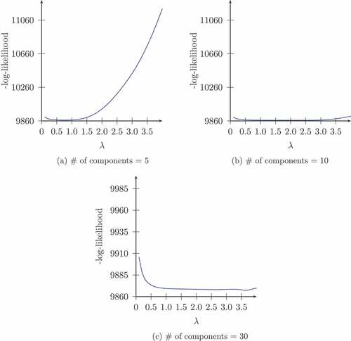
A possible explanation for this observation has to do with the fact that for a value of $\lambda$ as small as 1, the probability mass function of the Poisson random variable is approximately 0 for a number of arrivals greater than 5.

$\frac{{\lambda }^l{e}^{-\lambda }}{l!}\approx 0(\mathrm{f}\mathrm{o}\mathrm{r}l>5\mathrm{w}\mathrm{h}\mathrm{e}\mathrm{n}\lambda =1).$

In this case,

$\frac{{\lambda }^l{e}^{-\lambda }}{l!}\frac{1}{\sigma \sqrt{2\pi }}\mathrm{e}\mathrm{x}\mathrm{p}\left\{-\frac{{(y(t)-\mu -kl)}^2}{2{\sigma }^2}\right\}\approx 0\mathrm{\forall }\mu ,k.$

The above identification problem is different from the problem discussed in the paper by Honoré (1998) because we are working with jumps of a constant size $k$.

To mitigate the observed identification problem, the number of components of the mixture is determined in an adaptive way while evaluating the likelihood function. For a given vector of parameters, the number of components is chosen to be the minimum value of $m$ such that

$\left|\sum _{j=0}^{m}p(Q=j)-1\right|<\in ,$

for a very small $\in$.

Another identification issue commonly observed in finite mixture models is the potential existence of multiple maxima of the log-likelihood function. We tried to deal with this problem by estimating the model repeatedly with randomly chosen starting values and chose the estimates that correspond to the highest maximum.

6.1.2. Model with jumps of two different sizes

The techniques used above also apply to this model.

6.1.2.1. Moments

The mean is given by

(94) $\mathbb{E}[f(t)]=f(0)+\mu t+(k_1{\lambda }_1+k_2{\lambda }_2)t.$(94)

The variance is given by

(95) $\mathbb{V}\mathrm{a}\mathrm{r}[f(t)]=({\sigma }^2+k_1^2{\lambda }_1+k_2^2{\lambda }_2)t.$(95)

Though the distribution of $f(t)$ may not have a closed form, the moments of the distribution can be found using the characteristic function technique or the moment generating function technique as previously described. The characteristic function can be shown to be of the form

(96) ${\mathrm{\Phi }}_{f(t)}(u)=e^{iu(f(0)+\mu t)-\frac{{\sigma }^{2}t{u}^2}{2}+{\lambda }_{1}t(e^{i{k}_{1}u}-1)+{\lambda }_{2}t(e^{i{k}_{2}u}-1)}.$(96)

This entails the following expression for the first moment

(97) $\mathbb{E}[f(t)]=-i{\mathrm{\Phi }}_{f(t)}(0)$(97)

(98) $=f(0)+\mu t+({\lambda }_1{k}_1+{\lambda }_2{k}_2)t.$(98)

Of course, we have previously derived this expression directly. Similarly, we know that all the moments can be found from the characteristic function. The second noncentered moment is given by

(99) $\mathrm{\Phi }{{ }^{\mathrm{\prime }\mathrm{\prime }}}_{f(t)}(u)=-\mathbb{E}[f(t{)}^2{e}^{iuf(t)}].$(99)

Moreover, it is easily found that

(100) $\varphi {{ }^{\mathrm{\prime }\mathrm{\prime }}}_{f(t)}(0)=(-{\sigma }^{2}t-{\lambda }_1{k}_1^{2}t-{\lambda }_2{k}_2^{2}t)+(i(f(0)+\mu t)+{\lambda }_1{k}_{1}it+{\lambda }_2{k}_{2}it{)}^2.$(100)

Therefore, we obtain

(101) $\mathbb{V}\mathrm{a}\mathrm{r}[f(t)]=({\sigma }^2+{\lambda }_1{k}_1^2+{\lambda }_2{k}_2^2)t.$(101)

This is the same expression as previously found. Hence, all the moments can be found from the characteristic function without knowledge of the distribution of the process $\{f(t){\}}_{t\ge 0}$. Those moments can subsequently be used to estimate the parameters by GMM.

6.1.2.2. Density

If we want to estimate the model by Maximum Likelihood we need at least an approximation of the full density of the model. Fortunately, we can again discretize the model by the Euler method and use the resulting equation to approximate the density of the model.

The discretized version of Equation 48(48) $df(t)=\mu dt+\sigma dW(t)+k_{1}d{N}_1(t)+k_{2}d{N}_2(t),$(48) is the following:

(102) $f(t_j)-f(t_{j-1})=\mu \mathrm{\Delta }t+\sigma \sqrt{\mathrm{\Delta }t}z+k_1(N_1(t_j)-N_1(t_{j-1}))+k_2(N_2(t_j)-N_2(t_{j-1})).$(102)

Let $N_1(t_j)-N_1(t_{j-1})=Q_1(t_j)$, $N_2(t_j)-N_2(t_{j-1})=Q_2(t_j)$, and $f(t_j)-f(t_{j-1})=y(t_j)$, then

(103) $Q_1(t_j)\sim \mathrm{P}\mathrm{o}\mathrm{i}\mathrm{s}\mathrm{s}\mathrm{o}\mathrm{n}({\lambda }_1\mathrm{\Delta }t),Q_2(t_j)\sim \mathrm{P}\mathrm{o}\mathrm{i}\mathrm{s}\mathrm{s}\mathrm{o}\mathrm{n}({\lambda }_2\mathrm{\Delta }t)$(103)

and

(104) $y(t_j)|Q_1(t_j),Q_2(t_j)\sim \mathrm{N}(\mu \mathrm{\Delta }t+k_1{Q}_1(t_j)+k_2{Q}_2(t_j),{\sigma }^2\mathrm{\Delta }t).$(104)

The marginal distribution of $y_{t_j}$ is then

(105) $h(y(t_j))=\sum _{l=0}^{\mathrm{\infty }}\sum _{m=0}^{\mathrm{\infty }}p(Q_1(t_j)=l,Q_2(t_j)=m)h(y(t_j)|Q_1(t_j)=l,Q_2(t_j)=m)$(105)

(106) $=\sum _{l=0}^{\mathrm{\infty }}\sum _{m=0}^{\mathrm{\infty }}\frac{{({\lambda }_1\mathrm{\Delta }t)}^l{e}^{-{\lambda }_1\mathrm{\Delta }t}}{l!}\frac{{({\lambda }_2\mathrm{\Delta }t)}^m{e}^{-{\lambda }_2\mathrm{\Delta }t}}{m!}\frac{1}{\sigma \sqrt{\mathrm{\Delta }t}\sqrt{2\pi }}\mathrm{e}\mathrm{x}\mathrm{p}\left\{-\frac{{(y(t_j)-\mu \mathrm{\Delta }t-k_{1}l-k_{2}m)}^2}{2{\sigma }^2\mathrm{\Delta }t}\right\},$(106)

which takes the form of a mixture of an infinite number of normal distributions. The knowledge of the above density function makes the estimation of the parameters of the fundamentals process, via maximum likelihood, possible after choosing appropriate cutoff values that allow the approximation of the double sum as a finite sum.

6.2. Estimation of the remaining parameters

The remaining parameters will be estimated by the method of simulated moments (Gourieroux and Monfort, 1996) (MSM). Based on Equation 16(16) $f(t)=f(0)+\mu t+\sigma W(t)+kN(t),$(16) , the exchange rate can be written as

$s(t;\theta ,\alpha )=G[f(t;\theta );\alpha ],$

where $\theta$ is the vector of parameters that characterize the fundamentals process and $\alpha$ is an additional parameter that appears in the exchange rate process. Since there is no intersection between $\alpha$ and $\theta$, once we obtain the maximum likelihood estimate $\hat{\theta }$ of $\theta$ in the first step, we can generate draws for the fundamental process, $\{f(t;\hat{\theta })\}$. Those draws will be used subsequently to obtain draws for the exchange rate process using

$s(t;\alpha )=G[f(t;\hat{\theta });\alpha ]$

for given values of $\alpha$. Thus, in the second step, we will find an estimate of $\alpha$ that minimizes the distance between some moments of the simulated exchange rate and the corresponding moments of the observed exchange rate data. Let $M_T(\alpha )$ be such a column vector of moments and $W_T$ a weighting matrix. Then, the GMM estimator of $\alpha$ is obtained as

$\hat{\alpha }=\underset{\alpha }{argmin}{M}_T^{\prime }\left(\alpha \right)W_T^{-1}\left(\alpha \right)M_T\left(\alpha \right).$

6.3. Monte Carlo simulation

To assess the precisions of the estimates we have drawn 500 samples each of size 500 from the jump-diffusion process and from the exchange rate process. The parameters chosen are the following:

$\mu =0;\sigma =\sqrt{0.1};k=0.5;\lambda =2;\alpha =0.4;\mathrm{\Delta }t=1/52.$

For each sample, we estimate the parameters of the diffusion process. Then the estimates of the parameters of the diffusion process, the series $f$, and the initial and final values for $s$ are then used to estimate $\alpha$. The following figure (Figure 3) shows the sampling distribution of the parameter estimates.

Figure 3. Histograms of the estimates of the parameters of the jump-diffusion process.

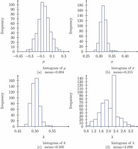
The Monte Carlo covariance matrix of the parameter estimates of the jump-diffusion process is the following

$\left(\begin{array}{cccccc}\hspace{0.17em}& \mu & \sigma & k& \lambda & \alpha \\ \mu & 0.01015& -0.00004& -0.00036& 0.00211& -0.00228\\ \sigma & -0.00004& 0.00010& 0.00001& -0.00006& -0.00002\\ k& -0.00036& 0.00001& 0.00013& 0.00000& -0.00011\\ \lambda & 0.00211& -0.00006& 0.00000& 0.20099& -0.05138\\ \alpha & -0.00228& -0.00002& -0.00011& -0.05138& 0.01513\end{array}\right)$

The above results show that we can estimate the parameters of the model with a high precision.

6.4. Application to monthly data on $f(t)$ and$s(t)$

We estimate the first model using monthly data from January 1972 to April 2018 for the US, Canada, and Japan. The data include the bilateral exchange rates between the US and the other two countries, the monetary aggregates (M1) for each country, and the industrial production index used as proxy for the Gross Domestic Product (GDP) of each country. The exchange rates and the US monetary aggregate originate from the Board of Governors of the Federal Reserve System and the other data come from the Organization for Economic Co-operation and Development (OECD). We present some summary statistics in Table 1.

Table 1. Summary statistics

Variable	Minimum	Maximum	Mean	Median	Standard Deviation
Canada
$\mathrm{\Delta }f$ ^a	−0.0469	0.0578	−0.0023	−0.0030	0.0150
$\mathrm{\Delta }log(s)$ ^b	−0.0601	0.1129	0.0004	0.0002	0.0148
Japan
$\mathrm{\Delta }f$	−0.1770	0.0874	−0.0013	−0.0012	0.0215
$\mathrm{\Delta }log(s)$	−0.1052	0.0807	−0.0019	−0.0001	0.0267

^a$\mathrm{\Delta }f$ is the first difference of the fundamental series, $f$, which is derived as $f=m-m^{\ast }-(y-y^{\ast })$ (Mark, 1995), $m$ is the log of the US monetary aggregate, $m^{\ast }$ is the log of the corresponding foreign monetary aggregate, $y$ is the log of the US industrial production index, and $y^{\ast }$ is the log of the foreign industrial production index.

^b$\mathrm{\Delta }log(s)$ is the percentage change in the value of the foreign currency. $s$ is expressed in units of foreign currency per US dollar.

As indicated in the table, the monthly changes in the fundamentals ($\mathrm{\Delta }f$) and in the log of the exchange rate ($\mathrm{\Delta }log(s)$) are on average small. Since the average change in the fundamentals is negative for both countries, the monetary aggregate (M1) and/or the industrial production index grew faster in those countries than in the US. However, the Canadian Dollar has slightly depreciated, while the Japanese Yen has slightly appreciated over the period.

Estimates of the parameters of the fundamental process are presented in Table 2.

Table 2. Estimates of the parameters of the fundamental process for Canada and Japan

	ABM			ABM with jump
Parameters	estimates	ste^a	p-value	estimates	ste	p-value
Model for Canada
$\mu$	0.0100	0.0081	0.2194	−0.0333	0.0077	0.0000
$\sigma$ ^b	0.0531	0.0017	0.0000	0.0493	0.0017	0.0000
$k$				0.0437	0.0094	0.0000
$\lambda$ ^b				0.1440	0.0969	0.1374
log-likelihood	1531.6049			1547.9094
AIC	−3059.2099			−3087.8188
BIC	−3050.5719			−3070.5429
Model for Japan
$\mu$	0.0100	0.0111	0.3669	−0.0070	0.0099	0.4796
$\sigma$ ^b	0.0747	0.0023	0.0000	0.0673	0.0020	0.0000
$k$				−0.1220	0.0126	0.0000
$\lambda$ ^b				0.0667	0.0387	0.0847
log-likelihood	1342.2636			1380.8993
AIC	−2680.5271			−2753.7985
BIC	−2671.8892			−2736.5227

^aste = standard error

^bAll the p-values are two-sided, but $\sigma$ and $\lambda$ are restricted to be positive. Thus, appropriate p-value for these variables should be half the values in the table.

^c$AIC=-2\ast \mathrm{l}\mathrm{o}\mathrm{g}-\mathrm{l}\mathrm{i}\mathrm{k}\mathrm{e}\mathrm{l}\mathrm{i}\mathrm{h}\mathrm{o}\mathrm{o}\mathrm{d}+2\ast \mathrm{n}\mathrm{u}\mathrm{m}\mathrm{b}\mathrm{e}\mathrm{r}\mathrm{o}\mathrm{f}\mathrm{p}\mathrm{a}\mathrm{r}\mathrm{a}\mathrm{m}\mathrm{e}\mathrm{t}\mathrm{e}\mathrm{r}\mathrm{s}$

^d$BIC=-2\ast \mathrm{l}\mathrm{o}\mathrm{g}-\mathrm{l}\mathrm{i}\mathrm{k}\mathrm{e}\mathrm{l}\mathrm{i}\mathrm{h}\mathrm{o}\mathrm{o}\mathrm{d}+log(n)\ast \mathrm{n}\mathrm{u}\mathrm{m}\mathrm{b}\mathrm{e}\mathrm{r}\mathrm{o}\mathrm{f}\mathrm{p}\mathrm{a}\mathrm{r}\mathrm{a}\mathrm{m}\mathrm{e}\mathrm{t}\mathrm{e}\mathrm{r}\mathrm{s}$

All the reported p-values are two-sided, but $\sigma$ and $\lambda$ are restricted to be positive. Thus, the appropriate p-value for these variables should be half the values in the table. As result, at a 5% level the jump size $k$ and $\lambda$ are both significantly different from 0 for Japan, which is evidence of the presence of jumps in the data for this country. For Canada, only the jump size, $k$, is statistically significant. However, both the Akaike Information Criterion (AIC) and the Bayesian Information Criterion (BIC) suggest that the model that accounts for jumps fits the data better than the usual diffusion process for both countries.

Since the process with jumps and the one without jumps are nested, the likelihood ratio test would be an alternative way of comparing them. Although the log-likelihood for the jump process is clearly greater than the log-likelihood of the usual diffusion, the p-value calculated using the chi-square distribution as the asymptotic distribution of the likelihood ratio statistic may not be correct because one of the regularity conditions is violated. Under the null hypothesis of no jumps in the process, one of the parameters, the intensity of the Poisson process, $\lambda$, falls on the boundary of the parameter set. Since the mean of the jumps is given by the product of the size of the jumps ($k$) and the intensity of the Poisson process ($\lambda$), on average the change in the fundamentals jumped up by 0.0063 for Canada and down by 0.008 for Japan.

Table 3 includes the estimates of $\alpha$ for both countries.

Table 3. Estimates of $\alpha$ for Canada and Japan

	estimate	ste^a	p-value	J-stat	J-stat p-value
Canada	1162.9387	183.9531	6.3219	51.6241	0.0000
Japan	212.3611	5.7941	36.6513	557.0297	0.0000

^aste = standard error

Although the model that allows for the existence of jumps fit the data of the fundamentals series better, the estimates of $\alpha$ for both countries and the GMM J-statistic are large. This result may be due to the method used to estimate $\alpha$. The exchange rate derived in the paper is a complicated function of the fundamentals, its parameters, and $\theta$. The existence of an approximate density for the fundamentals process allows us to efficiently estimate its parameters. However, neither the density nor the moments of the exchange rate process are available.

7. Conclusion

The paper provides a theoretical framework for exchange rate modeling in continuous time that accounts for the existence of jumps in exchange rate series. We derived the approximate relationship between the exchange rate and the process describing the macroeconomic fundamentals for two different specifications. Our empirical analysis shows that the modeling of jumps lead to a better fit of the fundamentals data for Canada and Japan. However, the estimation of the parameters that are not included in the fundamentals process is somewhat complicated and should be the object of further research.

Disclosure statement

No potential conflict of interest was reported by the author(s).

Additional information

Funding

The authors received no direct funding for this research.

References

- Akgiray, V., & Booth, G.G. (1988, November). Mixed diffusion-jump process modeling of exchange rate movements. The Review of Economics and Statistics, 70(4), 631–23. https://doi.org/10.2307/1935826
- Ball, C.A., & Torous, W.N. (1985, March). On jumps in common stock prices and their impact on call option pricing. The Journal of Finance, 40(1), 155–173. https://doi.org/10.1111/j.1540-6261.1985.tb04942.x
- Barrow, R. A., & Rosenfeld, E. R. (1984). Jump risk and the intertemporal capital asset pricing model. Journal of Business, 57(3), 337–351. https://doi.org/10.1086/296267
- Bates, D. S. (1996). Jumps and stochastic volatility: exchange rate processes implicit in deutsche mark options. The Review of Financial Studies. 9(1), 69–107. https://doi.org/10.1093/rfs/9.1.69
- Cheung, Y.-W., Chinn, M. D., & Pascual, A.G. (2005). Empirical exchange rate models of the nineties: are any fit to survive? Journal of International Money and Finance, 24(7), 0 1150–1175. https://doi.org/10.1016/j.jimonfin.2005.08.002
- Cont, R., & Tankov, P. (2004). Financial modeling with jump processes. Chapman & Hall/CRC.
- Erdemlioglu, D., Laurent, S., & Neely, C.J. (2015). Which continuous-time model is most appropriate for exchange rates? Journal of Banking and Finance, 61(2), 255–268. https://doi.org/10.1016/j.jbankfin.2015.09.014
- Ficura, M. (2015). Modeling jump clustering in the four major foreign exchange rates using high-frequency returns and cross-exciting jump processes. , 25, 0 208–219. https://doi.org/10.1016/S2212-5671(15)00731-5
- Gourieroux, C., & Monfort, A. (1996). Simulation-based econometric method. Oxford University Press.
- Hansom, F. B. (2007). Applied stochastic processes and control for jump-diffusions: modeling, analysis, and computation. Society for Industrial and Applied Mathematics. https://epubs.siam.org/doi/book/10.1137/1.9780898718638
- Honoré, P. (1998). Pitfalls in estimating jump-diffusion models. Unpublished.
- Ito, K. (1944). Stochastic integral. Proceedings of the Imperial Academy, 20(9), 519–524. https://doi.org/10.3792/pia/1195572786
- Jorion, P. (1988). On jump processes in the foreign exchange and stock markets. The Review of Financial Studies, 1(4), 427–445. https://doi.org/10.1093/rfs/1.4.427
- Mark, N. (1995). Exchange rates and fundamentals: evidence on long-horizon predictability. American Economic Review, 85(1), 201–218. https://www.jstor.org/stable/2118004
- Moh, Y.-K. (2006). Continuous-time model of uncovered interest parity with regulated jump-diffusion interest differential. Applied Economics, 38(21), 2523–2533. https://doi.org/10.1080/00036840500427809
- Richard, A. M., & Rogoff, K. (1983, February). Empirical exchange rate models of the seventies: Do they fit out of sample? Journal of International Economics, 14(1–2), 2–24. https://doi.org/10.1016/0022-1996(83)90017-X
- Situ, R. (2005). Theory of stochastic differential equations with jumps and applications. Springer.