On the goodness-of-fits of the generalized lambda distribution on high-frequency stock index returns

Abstract

In this paper, we investigate the goodness-of-fit of the flexible four-parameter generalized Lambda Distribution (GLD) for high-frequency 5-min returns sampled from the DJI30 Index. Applying Moment Matching (MM) and Maximum Likelihood Estimation (MLE) techniques, we highlight the significance of the higher-order parameters of the GLD distribution to depict the asymmetric and fat-tailed behaviour observed in high-frequency returns data. We also show and explain why the MLE consistently outperforms the MM; especially in the presence of “outliers”. Finally, we use lambda-space scatterplots to introduce, clarify and discuss additional stylized facts of high-frequency index returns not found in the extant high-frequency literature.

Keywords:

• Maximum likelihood
• moment matching
• generalized lambda distribution
• high-frequency
• Goodness-of-fit
• higher moments

JEL Classification:

• C52
• C58
• C59

1. Introduction

The fact that the normal distribution is inadequate in depicting the observed asymmetric and fat-tailed behaviour of financial returns is an ubiquitous fact in the extant finance literature and requires no further statistical rigour to prove otherwise, especially when it comes to depicting high-frequency financial returns (Bai, 2000; Dacorogna & Pictet, 1997; Dias & Embrechts et al., 2004; Fama, 1965). The literature has been quite exhaustive in the quest for an appropriate distribution. The main bane, however, has been to find a probability distribution that will adequately capture both the dispersion and also the bias and fat-tailedness observed in high-frequency finance (Su, 2007b). The various alternatives range from the parametric four-variable generalized lambda distribution (GλD; Freimer et al., 1988; Karian & Dudewicz, 2000; King & MacGillivray, 1999; Lakhany & Mausser, 2000; Okur, 1988; Öztürk & Dale, 1985; Ramberg & Schmeiser, 1974; Su, 2005b) to various non-parametric kernel density estimators (Silverman, 1986; Wegman, 1972). Of the many alternatives considered to-date, the four-parameter GλD has been consistent in providing the flexibility and robustness warranted in depicting the first four moments as when compared with the other alternatives. The four-parameters of the GλD are λ₁ (location), λ₂ (scale), λ₃ and λ₄ (shape) parameters (the latter two higher-order parameters relate to the lower and upper tails, respectively, and in combination can be transformed into the skewness and kurtosis measures).

One of the earliest works on fitting the four-parameter GλD distribution to returns data is by Ramberg et al. (1979). This was followed by the seminal monograph of Karian and Dudewicz (2000) from which many recent studies have explored different parameter estimation approaches to fitting empirical data. Since then, a number of studies have sought to improve the formulation of the GλD to fit the empirical data even better. For instance, to find robust moments in the GλD estimation, Chalabi et al. (2012), Chalabi et al. (2010), and Scott and Wuertz et al. (2012) express the location and scale parameters implicitly as the median and interquartile range of the distribution. The motive stems from, as noted by the authors, the difficulty in the parameter estimation of the GλD as the distributional shapes change rapidly by varying the parameters in the different regions of the two shape parameters, i.e. in the four regions of the λ₃-λ₄ lambda-space as per Figure 1. The authors further state “in particular, the support of the distribution can change with the value of the parameters from being the whole real line to an interval which is infinite in only one direction”, hence recommending fitting to be undertaken only within regions where such dramatic changes do not take place (Chalabi et al., 2010, p. 3). Using a different approach, Van Staden et al. (2014) developed a quantile-based generalized Pareto (GP) formulation with a skewness-invariant measure of kurtosis so that both the skewness and kurtosis parameters could be studied independently.

Figure 1. FMKL-GλD Support Regions in λ₃-λ₄ space (Chalabi et al., 2012, 2010).

In parallel with the development in fitting algorithms, there has been a growing number of applications of the GλD to various financial data. For instance, Corrado (2001) extends the GλD by developing a multivariate version to model the non-lognormal distribution of observed option prices. The author chose the GλD because of the wide range and flexibility of the skewness and kurtosis values realisable. Pfaff (2016) also employed the GλD in additon to the generalized hyperbolic distribution (GHD) and its special cases, namely: hyperbolic distribution (HYP), normal inverse Gaussian distribution (NIG), to fit the Hewlett-Packard (HWP) stock returns data. Corlu et al. (2016) investigate how well five alternative distributions (i.e. skewed Student t, GλD, Jonhson system, NIG, and g-and-h) fit stock data over the period of 1979 to 2014. They find the GλD to be the best alternative to depict daily equity returns of 19 indices from Europe, North and South America, Asia, and Africa. Also, Maghyereh and Al-Zoubi (2008) make use of extreme value theory (EVT) to scrutinize asymptotic tail distribution of daily returns in the Gulf region. The authors use the “Peaks-Over-Threshold” (POT) model to estimate the tails of the innovational distribution as they examine extreme returns. The models exploit tail behaviour and the Gulf equity markets can rely on EVT-based risk model in their risk assessment, as argued by the authors. Furthermore, Marsani et al. (2017) also examine the tail properties of the Kuala Lumpur composite index (KLCI) using GλD, generalized extreme value (GEV), generalized logistic (GL), generalized Pareto (GP), and Pearson (PE) distributions. Having estimated parameters by the L-moment method and using the k-sample Anderson Darling goodness-of-fit test, they find that the GλD outperforms all the four other distributions for the weekly maximums and minimums.

The GλD has been applied increasingly to data other than equity-related data as well. For example, Corlu and Corlu (2015) use daily closing price of nine different currencies in terms of the US dollar they investigate the performance of GλD via a numerical study against the skewed t distribution, the unbounded Johnson family of distributions, and the normal inverse Gaussian (NIG) distribution. They conclude that the GλD can be a good choice in various financial applications where modelling of the fat-tail behaviour is of great importance. Similarly, albeit mathematically revolutionary, Chalabi et al. (2012) fit USD/CHF exchange rate tick data for 2004, 2006, 2008 and 2012 to the GλD having derived robust estimators for the moments of the original model. Among others, the authors indicate the directness of this process which in turn could simplify the formulae to express value-at-Risk (VaR), expected shortfall (ES), and other tail indices. Furthermore, Tarsitano (2004) models the distribution of income over a population using the GλD on the premise that personal income distributions could adequately be described by the quantile function. For emerging European countries, Heinz and Rusinova (2015) prove the presence of heavy tails in the exchange market pressure (EMP) index through the use of Extreme Value Theory (EVT). They opine that disregarding these tail properties have the tendency to underestimate tail events.

In addition to the number of studies modifying the original formulation of the GλD and those applying the formulations to various financial data to test the appropriateness of the various versions of the same, there are also a number of studies that have investigated the adequacy of alternative estimations methods of the GλD itself. Corlu and Meterelliyoz (2016) used moment matching, L-moments, least-squares, quantile matching, maximum likelihood, the star-ship, and the genetic algorithm methods to compare the goodness-of-fits in estimating the FMKL-GλD. Each method was applied on daily exchange rates of eight currencies. However, the ensuing results were more varied than they were similar. Chalabi et al. (2010) and Scott and Wuertz et al. (2012) perform a Monte Carlo simulation closely resembling the returns of the NASDAQ-100 index and find the MLE to be reliable for small samples and heavy-tailed returns over maximum spacing, goodness-of-fit, and histogram binning approaches. Further, Mahdizadeh and Zamanzade (2019) examine the heavy-tails of the German Stock Index (DAX) using the Cauchy distribution. As in both Mahdizadeh and Zamanzade (2019) and Mahdizadeh and Zamanzade (2017), a battery of goodness-of-fit tests were performed. The tests perform better against the Gaussian distribution.

The extant literature suggests that there is a large authorship on the applications of the GλD to fit financial and economic low-frequency returns data. However, studies investigating the performance of the GλD estimations approaches for high-frequency financial data are sparse with the exception of Chalabi et al. (2012). This paper endeavours to fill this gap by investigating the shape distributions of 5-min high-frequency data as per the DJI30 Index (from January 2001 to December 2016) using the Freimer, Kollia, Mudholkar & Lin generalized Lambda distribution (FMKL-GλD) and both estimation methods of Moment Matching (MM) and Maximum Likelihood Estimation (MLE).

Our present study adds to the extant literature in three explicit ways. First, as stipulated earlier, studies that have employed the GλD have largely used low-frequency financial data. The use of tick data is almost absent save Chalabi et al. (2012) who apply their robust sample moments estimator to tick exchange rate data. Therefore, the paper attempts to increase literature on distribution of tick index data with an index comprising many prominent companies in the world. Second, as we sample the data as monthly 5-min log-return series, the non-stationarity in the price generating process is implicitly addressed. Hence, the inherent non-stationarity in a simple and indirect manner and makes the subsequent estimations and findings appropriate and relevant. Our choice of the size of each sample is also informed by the fact that in our preliminary analysis of the data the FMKL-GλD fit is rejected for the whole sample period (i.e. 5-mins intraday DJI30 Index from January 2001 to December 2016). Third, by taking the data sample from 2001 to 2016, the paper also explicitly includes the span of the Global Financial Crisis (GFC), particularly the year 2008, within the overall sample period. Thus, not only is the data up-to-date, but also covers both the pre- and post-GFC periods for subsequent comparisons. In addition, with a special focus on the 12 months in 2008, the paper highlights the GFC-affected shape distributional properties as per the FMKL-GλD. The associated time series plots of GλD parameters offer a rare insight into the evolution of the DJI30 return distribution over the GFC. Also λ₃-λ₄ lambda-space plots further describe the support regions for the fitted parameters during the crisis period which may be useful for risk estimates and decision-making.

In summary, in this paper, the extant empirical research around the generalized lambda distribution is further broadened so as to encompass high-frequency equity markets utilising the distributions and methods developed in Chalabi et al. (2012). Our findings confirm that the MLE outperforms the MM in line with extant literature and that for both MM and MLE the observed anomalies in fits are concomitant with not only large and negative shape parameter estimates (i.e. λ₃ and λ₄) but also with poor overall goodness-of-fits (i.e. GoFs).

The remainder of this paper proceeds as follows: Section 2 is an overview of the GλD in the light of Ramberg and Schmeiser (1974) (RS-GλD) and Freimer et al. (1988) (FMKL-GλD) approaches, with focus on the latter. Sections 3.1 & 3.2 respectively detail the two methodologies of moment matching (MM) and maximum likelihood estimation (MLE) in fitting the dataset of the GλD. Section 4 describes the data and a preliminary analysis of the same. Section 5 presents the estimated GλD parameters and other empirical results. We close the paper with goodness-of-fits (GoFs) comparisons between the MM and MLE methods followed by concluding remarks with practical implications in Sections 6 & 7 respectively.

2. Generalized Lambda Distribution (GλD)

The GλD was first introduced by Ramberg and Schmeiser (1974) as the inverse distribution function of Tukey’s lambda (TL) distribution. The Tukey’s lambda distribution, as in Hastings et al. (1947), has come to be known as the “Tukey-lambda” (TL) family of distributions and is defined as:

$X=Q\left(u\right)=\left\{\begin{array}{c}\frac{\left[u^{\lambda }-{\left(1-u\right)}^{\lambda }\right]}{\lambda },\lambda \ne 0\\ \frac{\mathrm{l}\mathrm{o}\mathrm{g}\left(u\right)}{1-u},\lambda \ne 0,\end{array}\right.(1)$

where $u$ is a uniform (0, 1) random variable and the transformation $Q\left(.\right)$, known as the quantile or percentile function, readily yields $Q\left(\alpha \right)$ as the $\alpha$ ^th quantile, 0 < α < 1, or 100α^th percentile of the distribution of X (see, Freimer et al., 1988).

Subsequently, a quantile generalization of the TL distribution known as the RS-GλD distribution was introduced by Ramberg and Schmeiser (1972, 1974); Ramberg et al. (1979) and is given as follows:

$F^{-1}\left(\rho |\lambda \right)={\lambda }_1+\frac{{\rho }^{{\lambda }_3}-{\left(1-\rho \right)}^{{\lambda }_4}}{{\lambda }_2}(2)$

where ρ are the probabilities (ρ$\in$[0, 1]), λ₁, λ₂ are the location and scale parameters, and λ₃, λ₄, the shape parameters jointly related to the strengths of the lower and upper tails, correspondingly. By restricting λ₁ = 0 and λ₂ = λ₃ = λ₄ = λ we obtain the one-parameter TL Chalabi et al. (2010) formulation.

The more recent Freimer et al. (1988), Freimer et al. (1988)—FMKL-GλD distribution (3) places only a single constrain of λ₂ > 0, i.e. the scale parameter is restricted to be positive. The fundamental motivation for the development of FMKL-GλD is that the distribution is well defined over all realisable λ₃ and λ₄ (Su, 2007a). The FMKL-GλD can be written as

$F^{-1}\left(\rho |\lambda \right)={\lambda }_1+\left[\frac{{\rho }^{{\lambda }_3-1}}{{\lambda }_3}-\frac{{\left(1-\rho \right)}^{{\lambda }_4-1}}{{\lambda }_4}\right]/{\lambda }_2(3)$

for 0 ≤ ρ ≤ 1.

In this study, comparison of methods moment matching and maximum likelihood is done using the FMKL-GλD since it has the property of being a valid distribution as long as λ₂ > 0, while the RS-GλD (2) is only valid for specified ranges of parameters. This means a fitting method using the RS-GλD will require a check to ensure the parameters are in the valid range, which makes programming more involved. Moreover, to allow a fair comparison, both fitting methods use exactly the same algorithm in obtaining initial values (Su, 2010). Also, as a preliminary suitability of the FMKL-GλD and other GλDs, for that matter, they are asymmetric. The four parameters of the various GλD types point to non-gaussianity. This stems from an extensive investigation by Karian and Dudewicz (2000), King and MacGillivray (1999), Ramberg and Schmeiser (1974), and Ramberg et al. (1979), etc. on the symmetry distribution version of the GλD given for λ₃ = λ₄; all parameter combinations do not yield valid density functions, an example is (4) Pfaff (2016). The probability density function of the GλD at $x=F^{-1}\left(\rho |\lambda \right)$ is given by:

(4) $f\left(x\right)=f\left(F^{-1}\left(\rho |\lambda \right)\right)=\frac{{\lambda }_2}{{\lambda }_3{\rho }^{{\lambda }_3-1}-{\lambda }_4{\left(1-\rho \right)}^{{\lambda }_3-1}}$(4)

wherefore parameter combinations of λ must yield $f\left(x\right)\ge 0$ and $\int f\left(x\right)dx=1$.

In an alternative parameterisation, Chalabi et al. (2012) reduce the GλD to a two-step estimation problem in fitting empirical data, wherein the location and scale parameters are estimated by their robust sample estimators. Furthermore, this approach works even in situations where the GλD moments do not exist. The authors, thus, converted the four parameter FMKL-GλD into a two parameter “asymmetry-steepness” formulation. The various methods for estimation of the optimal values for the parameter vector λ in the literature include, among others: moment-matching Ramberg et al. (1979); Ramberg and Schmeiser (1974); percentile-based Karian et al. (1996); histogram-based Su (2005a); goodness-of-fit Owen (1988); maximum likelihood (ML) and maximum spacing Cheng and Amin (1983); Ranneby (1984) and least squares (LS); Karvanen and Nuutinen (2008); Öztürk and Dale (1982), Öztürk & Dale (1985). In Su (2007a) the authors discourse two generic approaches to fitting generalized lambda distributions to data; using the discretized method and maximum likelihood estimation (or an approach that aims to provide a definite fit to the data set such as maximising the goodness-of-fit). Similar to Wang and Wang (2016) they preferred the maximum likelihood estimation to the former not just for its efficiency but also its likelihood to produce GλD with closer moments to the data set (Su, 2005a, 2007a; Wang & Wang, 2016).

2.1. FMKL-GλD distribution: classes and regions

Despite similarities in the definitions of the FMKL-GλD and RS-GλD parameters, their separate representations can present an array of shapes and their utilization in practice. For instance, Corlu and Meterelliyoz (2016) ascribed the preferability of the FMKL-GλD to the ease of use. The flexibility of GλDs exhibits itself more evidently with the FMKL-GλD. The four-parameter FMKL-GλD family is known for its high flexibility in generating distributions with a range of different shapes and has applications in studies as varied as in biology, physics, Monte Carlo, statistics and finance (Freimer et al., 1988; Jordan & Loeffen, 2013; Marcondes et al., 2020; Ridout, 2001; Zhu & Sudret, 2019).

The FMKL-GλD embodies unimodal, U-shaped, J-shaped, and monotone probability density functions (pdf’s). Freimer et al. (1988) assert that these can be symmetric or asymmetric with tails either smooth, abrupt or truncated, and long, medium, or short. These tail-shapes and density supports lead to the following categorisations: Class I (λ₃ < 1, λ₄ < 1) denoting unimodal densities with continuous tails and can be further subdivided with finite or infinite supports at the tails, Class II (λ₃ > 1, λ₄ < 1) referring to monotone pdf’s similar to those of exponential or ${\chi }_1^2$ distributions and with truncated left tails; Class III (1 < λ₃ < 2, 1 < λ₄ < 2) indicating U-shaped densities with left and right tails truncated; Class IV (λ₃ < 2, 1 < λ₄ < 2) representing the rare occurring S-shaped pdf’s with one mode and one antimode—both tails are truncated with the right rising sharply, and Class V (λ₃ > 2, λ₄ > 2) showing unimodal pdf’s with both tails truncated.

As mentioned above, the FMKL-GλD Class I (λ₃ < 1, λ₄ < 1) category can be further subdivided into four regions that can exhibit either a finite support (Region 3 with both tails bounded, Region 2 with the left tail bounded, Region 1 with the right tail bounded) or infinite support (Region 4 with both tails unbounded) as shown in Figure 1. Most notably and directly related to our study, Van Staden et al. (2014) and Karian and Dudewicz (2000, 2016) have also established that distributions with infinite support (i.e. their higher lambda parameters falling within Region 4 (λ₃ < 0, λ₄ < 0)) provide a better fit to empirical data as compared to those with finite supports. A full discussion of the range of the Regions 1 to 4 and the corresponding parameter supports are presented in Chalabi et al. (2012).

Hence, in this paper, we use the FMKL-GλD representation to examine the goodness-of-fits of the GλD using the method of moment matching and maximum likelihood for the DJI30 Index. Overall, we find that the DJI30 5-min monthly return distributions are of the Class I category (i.e. unimodal) and mainly fall within Region 4, as stated in Pfaff (2016), with the other three regions being occupied less frequently for both the MM and MLE fits over the sampled period.

3. Estimation techniques

After the pioneering works of Ramberg et al. (1979), Karian and Dudewicz (2000), and Karian et al. (1996), the method of moments, perhaps has been the most common approach in estimating the parameters of the GλD from empirical data. Since then, many other parameter estimation techniques have surfaced. In Section 2 we have indicated the various methods available in the literature; it would be useful to have all of them estimated and their performances compared. However, applying all the various methods mentioned will be an overkill against the focus of the present study; the remaining approaches are left for future research. Hence, in this paper, we only undertake and compare the method of moments matching (MM) and maximum likelihood estimation (MLE) using monthly sub-samples of our data. We present a summary of the Karian and Dudewicz (2000, 2016) MM algorithm in Section 3.1 and in Section 3.2 we briefly describe the MLE (Karian & Dudewicz, 2016, pp. 557–584) algorithm.

3.1. Method of moment matching

Given that a random variable Y has a non-normal distribution, we could attempt to approximate it by random variable $X$ that is $N\left(\mu ,\sigma 2\right)$ for some µ and σ² being mean and variance, respectively; (first two moments) chosen to match those of $Y$. However, the explicit restriction that X is normal (i.e. skewness = 0 and kurtosis = 3) provides no additional parameters to capture the third and fourth moments (Karian & Dudewicz, 2016). The popularity in the use of families of distributions with additional parameters to match not only the mean and variance but also the skewness and kurtosis stems from this implicit limitation of the normal distribution.

The family of GλDs is arguably a very good alternative to fix this drawback. To find a moment-based GλD fit to a given dataset X₁,X₂,X₃, …, X_n, the first four moments of X₁,X₂,X₃, …, X_n are determined and these set equal to their GλD (λ₁, λ₂, λ₃, λ₄) counterparts. The resulting equations are solved for λ₁, λ₂, λ₃, λ₄. If $X$ is GλD (λ₁, λ₂, λ₃, λ₄) with ${\lambda }_3>-1/4$ and ${\lambda }_3>-1/4$ (our data fully satisfy these), then its first four moments, α₁, α₂, α₃, α₄ (mean, variance, skewness, kurtosis, respectively) are given by a set of equations in Karian and Dudewicz (2016). In brief, the process is described in the following manner: start by setting λ₁ = 0; next obtain the non-central moments of the GλD (λ₁, λ₂, λ₃, λ₄); the finally derive the central GλD (λ₁, λ₂, λ₃, λ₄) moments. Thus, if X is a GλD (λ₁, λ₂, λ₃, λ₄) random variable, then Z = X − λ₁ is GλD (0, λ₂, λ₃, λ₄). If $Z$ is a GλD (0, λ₂, λ₃, λ₄), then E(Z^k), the expected value of Z^k is given by

(5) $E\left(Z^k\right)=\frac{1}{{\lambda }_2^k}\sum _{i=0}^k\left[\left(\begin{array}{c}k\\ i\end{array}\right){\left(-1\right)}^i\beta \left({\lambda }_3\left(k-i\right)+1,{\lambda }_{4i}+1\right))\right]$(5)

where β(a, b) is the beta function defined by

(6) $\beta \left(a,b\right)=\underset{0}{\overset{1}{\int }}{x}^{n-1}{\left(1-x\right)}^{b-1}dx$(6)

Then, the $k$-th GλD (λ₁, λ₂, λ₃, λ₄) moment exists if and only if ${\lambda }_3>-1/k$ and ${\lambda }_4>-1/k$. The proofs of these are provided in Theorem 3.1.4, Corollary 3.1.10, and Theorem 3.1.11 of Karian and Dudewicz (2016). These are not provided here for brevity reasons. It is clear from these equations that all four statistics depend on all four parameters and one has to solve a system of four non-linear equations to obtain the parameter estimates.

3.2. Method of maximum likelihood

The principle of the MLE states that the desired probability distribution is the one that makes the observed data “most likely” as originally postulated in Fisher (1922). This implies that one seeks the value of the parameter vector that maximizes the likelihood function as described in (7)—(11). Let $f(y|w)$ denote the probability density function (PDF) that specifies the probability of observing vector y given the parameter w. The likelihood function can be given as

(7) $l(w|y)=f(y|w)$(7)

(8) $\frac{1}{n}{X}^{T}u\left(\beta \right)=0$(8)

(9) $Lf(y|w)=\prod _{i=1}^{n}f(y|w)$(9)

(10) $\frac{\mathrm{\partial }L(w|y)}{\mathrm{\partial }{w}_i}=0$(10)

(11) $\frac{{\mathrm{\partial }}^{2}L(w|y)}{\mathrm{\partial }{w}_i^2}<0$(11)

where w = (w₁, …, w_k) is parameter vector defined on a multi-dimensional parameter space and y = (y₁, …, y_n) is a random sample data vector Myung (2003). Focardi and Fabozzi (2004) find the idea of the MLE highly intuitive as a principle of statistical estimation which, given a parametric model such as the GλD, prescribes choosing those parameters that maximize the likelihood of the sample under the model (Baum, 2007; Baum et al., 2003; Hansen, 1982; Hansen et al., 1996; Stock et al., 2002).

Contrary to least-squares estimation as a descriptive tool, MLE in particular, is preferred for many statistical modelling involving non-linearity with non-normal data and hence adequate for GλD. Given that the current literature is primarily concerned with providing definite fits to a dataset, Su (2007b) maintains that the MLE is usually the preferred method in comparing different approaches to fitting GλD to data. In addition to the efficiency of the MLE over the starship method, it also tends to produce GλD that has proximate first four moments to the data set. If the sample $y$ is independent and identically distributed (IID), then the likelihood is the product of individual likelihoods in (9). Assuming the log-likelihood function $lnL(w|y$) is differentiable, if $w_{MLE}$ (MLE estimate) exists, it must satisfy the partial differential equation called the likelihood equation in (10). A sufficient condition requires that $lnL(w|y$) is a maximum and not minimum. Hence, the shape of the function is convex. The empirical data in this study is fitted to the FMKL-GλD using the procedure described in the GLDEX R package (Su, 2007a).

4. High-Frequency DJI30 Data

Our data is the 5-min intraday Dow Jones Industrial Average (DJI30) spanning 4 January 2001 to 30 December 2016. Dow Jones Industrial Average is a benchmark for the stock market of USA; obtained from the Securities Industry Research Centre of Asia Pacific/Thomson Reuters Tick History (SIRCA/TRTH) database. To fully encapsulate the tail behaviour of the US stock market, we deem it fit to use high frequency rather than daily data based on the statistical principle that more data is preferred to less, ceteris paribus. Nonetheless, this may not always be true in the face of noise induced by microstructure frictions, such as price discreteness and bid-ask bounce effects, if unaccounted for (Aït-Sahalia et al., 2005; Bandi & Russell, 2006). To reduce the effect of noise, the most commonly used sampling frequency in the empirical literature range from 5-min intervals (T. Andersen et al., 1999; Barndorff-Nielsen & Shephard, 2002; Gençay et al., 2002) to long as 30 min (Andersen et al., 2003).

The DJI30 is selected for its rich history and fame as one of the best indices in the world. First published in 1896, index shows the results of trading on the stock market by 30 US large companies that participate in New York Stock Exchange and NASDAQ. The top five stocks in the index are 3 M, Boeing, Goldman Sachs, IBM, and UnitedHealth Group. The bottom five stocks, on the other hand, are Cisco Systems, Coca-Cola, General Electric, Intel, and Pfizer, classified according to market capitalisation. The 5-min price series was transformed into 5 min continuously compounded logarithmic returns, $r_t=ln\left(P_t\right)-ln\left(P_{t-1}\right)$ where $r_t$ and $P_t$ are log-return and price, respectively.

The full sample span (January 2001 to December 2016) is partitioned into monthly sub-samples of 5-min returns data to enable the capture of the implicit non-stationarity in the 5-min return series. The monthly sub-sample size was chosen over weekly or daily sub-sample sizes to ensure changing shape distributions to reflect the evolving dynamics inherent in the higher moment parameters. By doing so, we explicitly assume stationarity for the sub-sampled data. There is no optimal subsample period per se, but the monthly sub-samples provide a simple trade-off between sub-sample size and the sample data span. We subsequently filter the monthly sub-samples to remove overnight returns, winsorize at 99.99% to remove outliers, and also remove zero returns to reduce the kinkiness in the observed Q-Q plots.

5. Empirical results and analysis

5.1. Log-returns and moments of DJI30

The price plot, log-return plot, and descriptive statistics tables are presented as supplementary material¹ to maintain brevity of the paper, but we provide an explanation here. For most of the months the log-return plots show a variance in the neighbourhood of 0.02 to 0.06, outside of these we record a variance of 0.08 in March 2003. We have not recorded significant volatility clusters for these series. For shorter samples such as monthly data, it is not a surprise that we find no clusters. There is almost an equal distribution of positive and negative monthly means. We also find that most of the months have negatively skewed log-returns as against positively skewed ones. Recording only positive excess kurtosis values for all monthly log-returns, we deem the DJI30 heavy-tailed and many months platykurtic with excess kurtosis less than 0 albeit September 2008 with leptokurtic distributions.

5.2. Fitted GλD by methods of moment matching & maximum likelihood estimation

Table 1 depicts the monthly estimates of the GλD by methods of moment matching (MM) and maximum likelihood estimation (MLE) along with their goodness-of-fit tests, as well as regions of support for only 2008 selected from the years (2001, 2002, 2003, 2008, & 2009) in which the GλD captured all four regions of support (Regions 1, 2, 3, & 4). The year 2008 is selected because it also coincides with the peak of the recent Global Financial Crisis (GFC). The scale parameter λ₂ has been scaled by a factor of $\frac{1}{10000}$. Goodness-of-fit (GoF) tests used are the Kolmogorov-Smirnoff Resample (KS-R) and Kolmogorov-Smirnoff Distance (KS-D) tests. The KS-R test assesses the similarity between fitted distribution and actual data by sampling a proportion (for example, 90%) of the data and fitted distribution and calculating the KS-R p-value. This process is then repeated many times and the number of times the p-value is not significant (does not reject the null hypothesis that fitted distribution is from the GλD) is recorded and reported. Thus, the higher the number, the more confident we can be that the fitted distribution is reasonable Su (2007a). The KS-D, on the other hand, produce a statistic that is premised on the largest absolute difference between the hypothesized distribution (i.e. the GλD) and the empirical distribution function (edf) (i.e. the actual data points). It has often been described as quantification of the eyeball test (Gan et al., 1991; Karian & Dudewicz, 2000). The KS-R has a wider usage in modern works, and it is seen as more robust than KS-D, at least over its inclination to reject the null hypothesis. For a wide array of goodness-of-fit tests, see, Mahdizadeh and Zamanzade (2017) and Mahdizadeh and Zamanzade (2019), among others.

Table 1. MM and MLE GλD estimates for DJI30 Index log-returns (2008)

	GλD	Parameters					GλD	Moments
MM	λ1	λ2	λ3	λ4	GoF(%) λ3 − λ4		Mean	Var	Skew	Kurt
January	−0.4	0.1191	−0.0046	−0.0592	69.4	Region 4	0.07	0.03	0.2685	1.9412
February	−0.2	0.1706	−0.0021	−0.0338	94.4	Region 4	−0.04	0.01	0.1447	1.5388
March	−0.2	0.1474	−0.0295	−0.0496	91.1	Region 4	−0.002	0.02	0.1023	1.925
April	0.4	0.2258	−0.0361	0.021	88.1	Region 1	0.2	0.0074	−0.2498	1.4774
May	−2	0.2517	−0.0005	0.0466	0.00	Region 1	−2	0.005	−0.1796	0.9762
June	−0.7	0.1849	0.056	0.0211	75.7	Region 3	−0.5	0.008	0.1243	0.7626
July	−0.3	0.1426	−0.0148	−0.0535	93.5	Region 4	0.04	0.02	0.1918	1.8869
August	0.2	0.200	0.0086	−0.0123	60.90	Region 2	0.3	0.008	0.0884	1.247
September	−0.56	0.1166	−0.1218	−0.1471	72	Region 4	−0.2	0.04	0.2312	6.1392
October	−1.4	0.0463	−0.0307	−0.0666	91.3	Region 4	−0.6	0.2	0.1918	2.2074
November	−1	0.0534	0.0157	−0.034	92.6	Region 2	−0.00004	0.1	0.2488	1.55
December	−0.2	0.0919	−0.0175	−0.0404	92.8	Region 4	0.03	0.04	0.1105	1.7144
MLE
January	−0.5	0.1284	−0.0445	−0.1064	87.1	Region 4	0.06	0.03	0.3866	3.3368
February.	−0.2	0.1728	−0.0185	−0.0454	94	Region 4	−0.03	0.01	0.1319	1.7887
March	−0.2	0.1474	−0.0245	−0.0547	89.7	Region 4	−0.008	0.03	0.1535	1.964
April	0.3	0.2285	−0.0402	0.0046	90.9	Region 1	0.1	0.007	−0.205	1.593
May	0.2	0.2306	−0.0088	0.0415	93.8	Region 1	0.02	0.006	−0.1975	1.0768
June	−0.7	0.1687	0.053	0.0241	94.4	Region 3	−0.5	0.01	0.103	0.7515
July	−0.1	0.1428	−0.0182	−0.0416	93.5	Region 4	0.07	0.02	0.1134	1.7358
Aug.	0.05	0.183	0.0083	−0.0336	90	Region 2	0.3	0.01	0.1865	1.4879
September	−0.8	0.1052	−0.0904	−0.135	93.9	Region 4	−0.2	0.05	0.3515	4.9319
October	−1	0.0478	−0.0615	−0.0885	93.3	Region 4	−0.5	0.2	0.1668	2.9171
November	−1	0.0535	0.001	−0.0557	91.4	Region 2	−0.3	0.1	0.2732	1.8578
December	−0.3	0.0931	−0.0732	−0.0997	91.3	Region 4	0.02	0.05	0.1753	3.3318

Note: λ₁, Mean & Variance values should be multiplied by 10⁻⁴. The KS-D test under MM record p-values of 0.00 and 0.02 for May and August, respectively, and none for MLE.

In the GoF column, we report only KS-R test statistic. We do not report the p-values of the KS-D test because they are all greater than 0.05 (i.e. indicating that GλD fits are not rejected), except for May and August (under MM) which are 0.00 and 0.02, respectively. At 5% significance level, the approximate percentage of the difference between the fitted and simulated distribution is reported for KS-R. These two reports are presented so that we can draw parallels for the two approaches. There were 16 different months out of 172 for the GλD via MM rejected by both KS-D and KS-R tests. Of these KS-R range from 0% to 70.30%. Notwithstanding, a few of the months for which the fit was accepted by both tests, some of KS-R’s fall below 70%. Unlike the MM fits, there are only 2 months, namely; August and December 2014, for which the MLE fits are rejected by both KS-D and KS-R tests, rejection in December 2014 here coincides with that of MM fit. However, MM records an adequacy value of 67.10% in August 2014 instead of 55.10% for MLE fit. The MLE fits record a least GoF of 59.80%. Quantile-quantile (Q-Q) plots are another way of assessing the adequacy of fits pictorially. For further reading see, Kolmogorov (1933), Su (2007b), Karian and Dudewicz (2000), Lakhany and Mausser (2000), and Babu and Feigelson (2006).

Further, in Figures 2 and 3, we present a select number of monthly histograms and Q-Q plots of the MM & MLE GLD fits (2008) falling in Regions 1, 2, 3, and 4 to provide a succinct comparison of the goodness-of-fits between MM and MLE. In Figure 2 are plots from May 2008 in Region 1, August 2008 in Region 2, June 2008 Region 3, and July 2008 Region 4 for MM; in ascending order of goodness-of-fit (clockwise). In May 2008, the GλD was rejected, absolutely for Region 1 failing to capture the tails; denoted by very poor histogram and Q-Q plot. For August 2008, the inadequacy (60.90%) seems to have arisen from high negative values observed in these plots. Large outliers in both regions have adverse effects on the overall fits. However, in June 2008 (Region 3) the fit is adequate at 75.7% with positive parameter values but this is topped by July 2008 (Region 4) with 95.5% adequacy albeit negative parameter values. For June 2008 (Region 3) the two large outliers had an adverse effect on the fit unlike the latter (July 2008 (Region 4)) with much smaller outliers.

Figure 2. Histograms and Q-Q plots of MM-GλD for selected months (2008): May/Region 1, August/Region 2, June/Region 3, and July/Region 4.

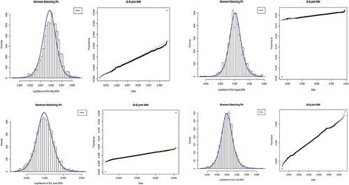
Figure 3. Histograms and Q-Q plots of MLE-GλD for selected months (2008): April/Region 1, August/Region 2, June/Region 3, and February/Region 4.

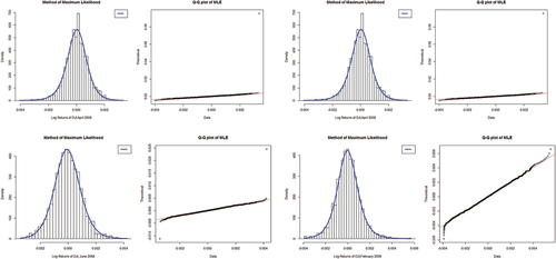
For MLE in Figure 3 we shown the months of April 2008 in Region 1, August 2008 in Region 2, June 2008 Region 3, and February 2008 in Region 4 (in ascending order of goodness-of-fit; clock-wise). In April and August 2008 (90.90% and 90%) one outlier each had their respective leverages making the fits failing to capture the peak, having encapsulated both tails. The outlying pair in June 2008; for 94.40% adequacy the fit is skewed to the right due to an extreme positive value dwarfing its positive counterpart; nonetheless bagging the peakedness fit for the sampled data. Adjudged the best fit by Q-Q plot at 94% adequacy and right-skewed, February 2008 also has a good histogram. It is very clear that comparatively the MLE performs better than MM for the DJI30 Index. Both methods result in the same “Regional” placements though their parameters (λ’s) differ quite a bit.

6. Performance Comparison

It is imperative to note that a GλD with very similar mean, variance, skewness, and kurtosis to the actual data may still be a bad fit (Karian & Dudewicz, 2000; Lakhany & Mausser, 2000). Hence, Su (2007a, p. 6) recommends “in some cases, it may be desirable to choose a good distributional fit with the closest mean, variance, skewness and kurtosis to the data set so that the fitted distribution can be used for simulation studies to model the population of interest”. Hence, in this section, we do a time series visual comparison of the MLE and MM fits.

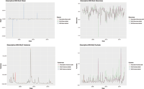
From the time series plots in Figure 5 we see how the descriptive mean, variance, skewness and kurtosis of the sample data have been subsumed under the mean, variance, skewness, and kurtosis of the two fitted distributions, except for mid-2003 where the variance of the sample data is markedly different from the others. Notwithstanding, for 16 and 2 months of MM and MLE fits, respectively, the GλD has been rejected. Thus, similarity of sample data moments with those of fitted distribution does not guarantee a better fit. More so, in Figure 4 we observe very large disparity in the magnitude of fitted moments and fitted lambda values. Hence, there is no clear correspondence between these two pairs of values.

Figure 4. GλD moments & parameters of DJI30 from January 2001 to December 2016.

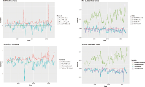
Figure 5. MM & MLE GλD moments overlaid with descriptive moments.

In the scatter plots of λ₄ against λ₃ in Figure 6 for MM (left pane) and MLE (left pane), the pairs (points) yielding rejected fits are in red colour. In Figure 6 we notice that the months of rejected fits have relatively high negative values for λ₃ and λ₄ for both MM and MLE, but especially the former. However, rejected fits are complementary and MLE is more robust than the MM. Nonetheless, extreme values of higher-order λ_s are more likely to be rejected by the GoFs. In other words, rejections are dictated by the extremeness of the higher-order shape parameters and is detected by the GoFs. Extreme values of higher-order shape parameters indicate the presence of outliers. We use a dashed diagonal line (in blue) to delineate the points of symmetry (i.e. points that lie on the diagonal line where λ₃ = λ₄). A perfectly symmetric distribution hardly ever occurs over the whole sample period for the two fitting methods except for MLE in December 2005; this single occurrence of perfect symmetry is depicted in purple on the MLE lambda-space plot.

Figure 6. Lambda (GλD) space of MM & MLE fits for DJI30 from 2001 to 2016.

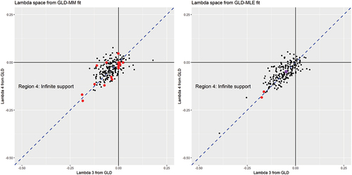
Given that the FMKL-GλD’s higher-order lambda estimates typically fall within Region 4, our corresponding estimates do not fully adhere to this behaviour as some of our fits fall outside Region 4 (as shown by Table 1 and in Figure 6). Furthermore, the higher-order lambda estimates are scattered close to the 45 degree diagonal. This highlights not only the non-stationarity of the data generation process but also that the presence of skewness and kurtosis in high-frequency returns is the norm. Furthermore, there seems to be no pattern in the Regions from which the rejections occur (see, Figures 6 and 7). For the MLE, both rejections come from Region 4 (August 2014 and December 2014); most of the lambda estimates fall in this region anyway. For the MM, the 16 rejections occur in Region 1 (March 2005), Region 2 (February 2003, July 2006, August 2008, and June 2011), none in Region 3, and Region 4 (September 2001, December 2001, September 2002, March 2004, September 2006, February 2007, May 2009, January 2010, October 2014, December 2015, and August 2015). The years for which all the Regions are occupied by the MM fits are 2001, 2002, 2003, 2008, and 2009. On the other hand, the years for which all Regions are occupied by the MLE fits are 2002 and 2008. These findings indicate that rejections can occur in all the regions and is likely driven by outlier-sensitivity rather than lambda-sensitivity, giving credence to the flexibility of the distribution for high-frequency returns. Also, the MLE algorithm is superior to the MM in accommodating outliers within the data.

Figure 7. Lambda (GλD) space of MM & MLE fits for DJI30 (2008). Note: The dot-points in red (May and August) indicate a rejection of the FMKL-GλD by the MM.

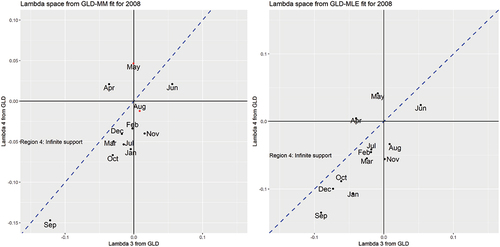
The Global Financial Crisis (GFC) occurred over the period between mid-2007 and early 2009 putting extreme stress into the world financial markets and banking systems. With US being the epicentre, the crisis peaked following the failure of the US financial firm Lehman Brothers in September 2008. To get a better insight to the shape of the monthly distributions around the month of the Lehman Brothers failure, we focus on the lambda-space plots for 2008 in Figure 7. The month of September is clearly an outlier as can be seen from the lambda-space plots with a negative implied skewness and a high implied kurtosis. The MM-fit shows this more clearly than the MLE-fit; indicating MM-fits are more sensitive to outliers occurring within the data. On the other hand, MLE fits are more sensitive to the “non-outliers” in the data as suggested by the greater dispersion or lower clustering of the dot-points in the right plot. The year 2008 was surely “bearish” with most of the months depicting negative returns. The MLE-lambda parameters are more homogeneous with less extreme MLE-lambda parameters on average than the MM-lambda parameters; once again giving credence to the superiority of the maximum likelihood method.

In the specific context of tail events modelling, we present in Table 2 the percentage difference (%-Diff) between the MM and MLE GλD higher-order moment estimates and the descriptive moments (benchmark), i.e. skewness and kurtosis. The underestimates (Under) and overestimates (Over) are listed under the “State” column.

Table 2. %-Differences of GλD Moments wrt Descriptive Moments (2008)

2008	MM				MLE
	Kurtosis		Skewness		Kurtosis		Skewness
	%-Diff	State	%-Diff	State	%-Diff	State	%-Diff	State
January	1.34E-06	Over	1.95E-05	Over	71.90	Over	43.99	Over
February	−1.10E-05	Under	−1.45E-03	Under	16.24	Over	−8.86	Under
March	2.39E-07	Over	1.02E-05	Over	2.03	Over	50.10	Over
April	−3.18E-07	Under	−2.16E-06	Under	7.82	Over	−17.94	Under
May	−3.49E-02	Under	−2.25E-01	Under	10.27	Over	9.69	Over
June	5.24E-07	Over	−4.99E-06	Under	−1.49	Under	−17.20	Under
July	1.06E-08	Over	−2.19E-06	Under	−8.01	Under	−40.88	Under
August	2.41E-07	Over	8.71E-06	Over	19.32	Over	110.96	Over
September	−8.80E-08	Under	−3.46E-07	Under	−19.67	Under	52.05	Over
October	−4.26E-07	Under	0.00	Null	32.15	Over	−13.02	Under
November	−2.77E-07	Under	3.09E-06	Over	19.82	Over	9.84	Over
December	−2.86E-07	Under	1.05E-05	Over	94.34	Over	58.69	Over

Under the MM approach, the higher-order moment %-differences are so tiny that one can safely assume that there are no significant differences between the MM-moments and the descriptive moments. This is not surprising as the MM approach minimizes the differences between the four moments, i.e. mean, variance, skewness and kurtosis. By definition, the MM method will always capture the descriptive moments with the least error. Unlike MM, the MLE moment estimates display large %-differences for most of the months in 2008. Skewness has %-differences ranging from −8.86% to 110.96% and kurtosis has %-differences ranging from −19.67% to 94.34%. However, these MLE large higher-order moment %-differences should not be seen as an inadequacy. The apparently large %-differences is a direct consequence of the MLE approach which maximizes the log-likelihood of the high-frequency returns within the relevant month. The MLE implicitly weighs the data around the median higher than the data around the tails, especially the outliers. This is further supported by the superior MLE-GoF test statistics. The MM method gives priority to the discrete four higher-order moments whereas the MLE method gives priority to the “shape-likelihood” of the overall data via the higher-order lambdas. Hence, the statement by Su (2007a, p. 6) that “in some cases, it may be desirable to choose a good distributional fit with the closest mean, variance, skewness and kurtosis to the data set so that the fitted distribution can be used for simulation studies to model the population of interest”.

7. Conclusions and practical implications

In the extant literature, we find that parametric density estimators are more consistent and efficient when compared to non-parametric density estimators. However, the high flexibility of four-parametric GλD distribution minimizes the inconsistency and inefficiency of a likely mismatch between the data and the distribution family assumed; that is to say the GλD addresses one of the biggest concerns about parametric density estimation—the reliability of the assumed functional form of the underlying distribution (Wang & Wang, 2016).

Using the FMKL-GλD fitted by MM on the one hand and MLE on the other, we identified the regions of support, periods of symmetry or otherwise, periods of goodness-of-fit or otherwise, and close matches between the sample data moments and the fitted distribution moments. To accomplish these, data was sub-sampled on a monthly basis to maintain stationary and homogeneity. We then showed that the MLE fitted FMKL-GλD captures realistically the tail behaviours (skewness and kurtosis) of the DJI30 5-min log-returns for the period from January 2001 to December 2016; with rejections for August and December 2014 only, whilst the alternative MM fits recorded rejections for 16 different months which were scattered across the four regions of support. This is due to the MM method giving priority to the four higher-order descriptive moments of the returns data and the MLE method giving priority to the likelihood of the “shape” of the empirical density of the same data. The results are in line with the extant literature that the MLE fits of the FMKL-GλD distribution perform better than the MM alternative (Su, 2005a, 2007a; Wang & Wang, 2016).

Our findings show that the four-parameters of the GλD of λ₁, λ₂ (location and scale parameters), λ₃, and λ₄ (shape parameters) are able to capture the shape of the 5-min return distributions consistently and efficiently for the DJI30 index for the monthly sub-samples under study. In addition, these four-parameters are also easily mapped into the first four descriptive moments, i.e. mean, variance, skewness and kurtosis. This inherent feature of the GλD distribution and its ease of fit will prove invaluable to any study in finance where the first four moments of asset return-distributions are relevant or required.

In terms of practical implications, regardless of which method (MM or MLE) fits the GλD distribution to the data, important ramifications can be drawn. Equity managers and investors who base their risk estimates and analysis on the first two descriptive moments (i.e. expected returns and variance) unknowingly carry significant levels of higher-order risk, among others; unsafe bets, unreliable forecasts, underestimating losses, as well as implicitly underestimating the number of assets to include in an optimal portfolio to mitigate unsystematic risk. These consequences stem from ignoring the additional information that the GλD distribution captures, i.e. the higher-order shape parameters directly allow for the presence of the higher-order moments (i.e. skewness and kurtosis) in asset return distributions. Furthermore, as a member of a family of stable distributions, diversification assuming the GλD considerably increases the number of stocks included in a portfolio in order to achieve the desired level systematic risk as when assuming the normal distribution (Young & Graff, 1995).

Additionally for portfolio risk management, the downside risk measures such as VaR and ES based on estimates using higher moments can also be useful for equity managers and investors. This becomes even more crucial in light of turbulent market conditions such as during the recent GFC. Given that the VaR and ES are tail measures, the normal distribution is by definition deficient in depicting the fat-tailed or extreme downside risks. In contrast, the GλD distribution allows for these tail parameters, hence its widespread use (like other asymmetric distributions) for calculating VaR and ES (Owusu Junior & Alagidede, 2020, 2020). Thus, not only are reductions of unsystematic risk fostered, but the overall portfolio risks are also more realistically measured and mitigated to ensure superior risk management of equity portfolios.

For future studies, goodness-of-fit tests can be expanded to include the fourteen tests performed in Mahdizadeh and Zamanzade (2017) and Mahdizadeh and Zamanzade (2019). This should provide a better understanding of the performance of not just the GλD but also financial assets under non-Gaussian assumptions. In addition, it will be insightful to compare the fitting performance using some Monte Carlo simulation, and then comparing the fitting results using mean absolute bias (MAB) and mean square error (MSE) measures for robustness reasons.

Ethical approval

No ethical approval was needed for this study.

Informed consent

No consent was needed from a third party for any portions of this study

Disclosure statement

No potential conflict of interest was reported by the authors.

Supplementary Material

Supplemental data for this article can be accessed online at https://doi.org/10.1080/23322039.2022.2095764

Additional information

Notes on contributors

Peterson Owusu Junior

Peterson Owusu Junior: Conceptualisation, Methodology, Software, Data curation, and Writing - original draft, Review, and Editing. Nagaratnam Jeyasreed-haran: Conceptualisation, Methodology, Data, Validation, Writing, and Review. Imhotep Paul Alagidede: Supervision, Review, and Editing.

Notes

1. https://drive.google.com/file/d/1ExvLOJ0mg-pxsxFLN026kQlBovtTk8El/view?uspsharing

References

- Aït-Sahalia, Y., Mykland, P. A., & Zhang, L. (2005). How often to sample a continuous-time process in the presence of market microstructure noise. The Review of Financial Studies, 18(2), 351–20. https://doi.org/10.1093/rfs/hhi016
- Andersen, T., Bollerslev, T., Diebold, F. X., & Labys, P. (1999). The distribution of exchange rate volatility. Technical report, National Bureau of Economic Research.
- Andersen, T. G., Bollerslev, T., Diebold, F. X., & Labys, P. (2003). Modeling and forecasting realized volatility. Econometrica, 71(2), 579–625. https://doi.org/10.1111/1468-0262.00418
- Babu, G., & Feigelson, E. (2006). Astrostatistics: Goodness-of-fit and all that! In Astronomical Data Analysis Software and Systems XV ASP Conference Series, volume 351, 127–136.
- Bai, X. (2000). Beyond Merton’s utopia: effects of non-normality and dependence on the precision of variance estimaters using high-frequency financial data. PhD thesis, University of Chicago, Graduate School of Business.
- Bandi, F. M., & Russell, J. R. (2006). Separating microstructure noise from volatility. Journal of Financial Economics, 79(3), 655–692. https://doi.org/10.1016/j.jfineco.2005.01.005
- Barndorff-Nielsen, O. E., & Shephard, N. (2002). Econometric analysis of realized volatility and its use in estimating stochastic volatility models. Journal of the Royal Statistical Society: Series B (Statistical Methodology), 64(2), 253–280. https://doi.org/10.1111/1467-9868.00336
- Baum, C. F., Schaffer, M. E., and Stillman, S. . (2003). Instrumental variables and GMM: Estimation and testing. Stata Journal, 3(1), 1–31. https://doi.org/10.1177/1536867X0300300101
- Baum, C. F. (2007). Instrumental variables estimation in stata. Boston College.
- Chalabi, Y., Scott, D. J., & Würtz, D. (2010). The generalized lambda distribution as an alternative to model financial returns. Z¨urich and University of Auckland, Zürich and Auckland. Institut für Theoretische Physik
- Chalabi, Y., Scott, D. J., & Wuertz, D. (2012). Flexible distribution modeling with the generalized lambda distribution. MPRA paper 43333. Munich: Munich Personal RePEc Archive.
- Cheng, R., & Amin, N. (1983). Estimating parameters in continuous univariate distributions with a shifted origin. Journal of the Royal Statistical Society: Series B (Methodological), 45(3), 394–403. https://doi.org/10.1111/j.2517-6161.1983.tb01268.x
- Corlu, C. G., & Corlu, A. (2015). Modelling exchange rate returns: Which flexible distribution to use? Quantitative Finance, 15(11), 1851–1864. https://doi.org/10.1080/14697688.2014.942231
- Corlu, C. G., Meterelliyoz, M., & Tinic, M. (2016). Empirical distributions of daily equity index returns: A comparison. Expert Systems with Applications, 54, 170–192. https://doi.org/10.1016/j.eswa.2015.12.048
- Corlu, C. G., & Meterelliyoz, M. (2016). Estimating the parameters of the generalized lambda distribution: Which method performs best? Communications in Statistics-Simulation and Computation, 45(7), 2276–2296. https://doi.org/10.1080/03610918.2014.901355
- Corrado, C. J. (2001). Option pricing based on the generalized lambda distribution. Journal of Futures Markets: Futures, Options, and Other Derivative Products, 21(3), 213–236. https://doi.org/10.1002/1096-9934(200103)21:3<213::AID-FUT2_3.0.CO;2-H
- Dacorogna, M. M., & Pictet, O. V. (1997). Heavy tails in high-frequency financial data. SSRN. (No. 1996-12–11; Working Papers). Olsen and Associates. https://doi.org/10.2139/ssrn.939
- Dias, A., Embrechts, P. et al. 2004. Dynamic copula models for multivariate high-frequency data in finance, Manuscript. ETH Zurich. 81.
- Fama, E. F. (1965). The behavior of stock-market prices. The Journal of Business, 38(1), 34–105. https://doi.org/10.1086/294743
- Fisher, R. A. (1922). On the mathematical foundations of theoretical statistics. Philosophical Transactions of the Royal Society of London. Series A, Containing Papers of a Mathematical or Physical Character, 222, 309–368. https://doi.org/10.1098/rsta.1922.0009
- Focardi, S. M., & Fabozzi, F. J. (2004). The mathematics of financial modeling and investment management (Vol. 138). John Wiley & Sons.
- Freimer, M., Kollia, G., Mudholkar, G. S., & Lin, C. T. (1988). A study of the generalized tukey lambda family. Communications in Statistics-Theory and Methods, 17(10), 3547–3567. https://doi.org/10.1080/03610928808829820
- Gan, F., Koehler, K. J., & Thompson, J. C. (1991). Probability plots and distribution curves for assessing the fit of probability models. The American Statistician, 45(1), 14–21. https://doi.org/10.1080/00031305.1991.10475759
- Gençay, R., Ballocchi, G., Dacorogna, M., Olsen, R., & Pictet, O. (2002). Real-time trading models and the statistical properties of foreign exchange rates. International Economic Review, 463–491.
- Hansen, L. P. (1982). Large sample properties of generalized method of moments estimators. Econometrica: Journal of the Econometric Society, 50(4), 1029–1054. https://doi.org/10.2307/1912775
- Hansen, L. P., Heaton, J., & Yaron, A. (1996). Finite-sample properties of some alternative gmm estimators. Journal of Business & Economic Statistics, 14(3), 262–280. https://doi.org/10.1080/07350015.1996.10524656
- Hastings, C., Mosteller, F., Tukey, J. W., and Winsor, C. P. (1947). Low moments for small samples: A comparative study of order statistics. The Annals of Mathematical Statistics, 18(3), 413–426. https://doi.org/10.1214/aoms/1177730388
- Heinz, F. F., & Rusinova, D. (2015). An alternative view of exchange market pressure episodes in emerging Europe: An analysis using extreme value theory (EVT). SSRN Electronic Journal. In Working Paper Series (No. 1818; Working Paper Series). European Central Bank. https://doi.org/10.2139/ssrn.2628734
- Jordan, R. B., & Loeffen, M. P. (2013). A new method for modelling biological variation using quantile functions. Postharvest Biology and Technology, 86, 387–401. https://doi.org/10.1016/j.postharvbio.2013.07.008
- Karian, Z. A., Dudewicz, E. J., & Mcdonald, P. (1996). The extended generalized lambda distribution system for fitting distributions to data: History, completion of theory, tables, applications, the “final word” on moment fits. Communications in Statistics-Simulation and Computation, 25(3), 611–642. https://doi.org/10.1080/03610919608813333
- Karian, Z. A., & Dudewicz, E. J. (2000). Fitting statistical distributions: The generalized lambda distribution and generalized bootstrap methods. CRC Press.
- Karian, Z. A., & Dudewicz, E. J. (2016). Handbook of fitting statistical distributions with R. CRC Press.
- Karvanen, J., & Nuutinen, A. (2008). Characterizing the generalized lambda distribution by l-moments. Computational Statistics & Data Analysis, 52(4), 1971–1983. https://doi.org/10.1016/j.csda.2007.06.021
- King, R. A., & MacGillivray, H. (1999). A starship estimation method for the generalized distributions. Australian & New Zealand Journal of Statistics, 41(3), 353–374. https://doi.org/10.1111/1467-842X.00089
- Kolmogorov, A. (1933). Sulla determinazione empirica di una legge di distribuzione. Giornale dell’Istituto Italiano degli Attuari, 10(12.2), 1.
- Lakhany, A., & Mausser, H. (2000). Estimating the parameters of the generalized lambda distribution. Algo Research Quarterly, 3(3), 47–58.
- Maghyereh, A. I., & Al-Zoubi, H. A. (2008). The tail behavior of extreme stock returns in the gulf emerging markets: An implication for financial risk management. Studies in Economics and Finance, 25(1), 21–37. https://doi.org/10.1108/10867370810857540
- Mahdizadeh, M., & Zamanzade, E. (2017). New goodness of fit tests for the Cauchy distribution. Journal of Applied Statistics, 44(6), 1106–1121. https://doi.org/10.1080/02664763.2016.1193726
- Mahdizadeh, M., & Zamanzade, E. (2019). Goodness-of-fit testing for the Cauchy distribution with application to financial modeling. Journal of King Saud University-Science, 31(4), 1167–1174. https://doi.org/10.1016/j.jksus.2019.01.015
- Marcondes, D., Peixoto, C., & Maia, A. C. (2020). A survey of a hurdle model for heavy-tailed data based on the generalized lambda distribution. Communications in Statistics-Theory and Methods, 49(4), 781–808. https://doi.org/10.1080/03610926.2018.1549251
- Marsani, M. F., Shabri, A., & Jan, N. A. M. (2017). Examine generalized lambda distribution fitting performance: An application to extreme share return in Malaysia. Malaysian Journal of Fundamental and Applied Sciences, 13(3). https://doi.org/10.11113/mjfas.v13n3.599
- Myung, I. J. (2003). Tutorial on maximum likelihood estimation. Journal of Mathematical Psychology, 47(1), 90–100. https://doi.org/10.1016/S0022-2496(02)00028-7
- Okur, M. C. (1988). On fitting the generalized λ-distribution to air pollution data. Atmospheric Environment (1967), 22(11), 2569–2572. https://doi.org/10.1016/0004-6981(88)90489-1
- Owen, A. B. (1988). Empirical likelihood ratio confidence intervals for a single functional. Biometrika, 75(2), 237–249. https://doi.org/10.1093/biomet/75.2.237
- Owusu Junior, P., & Alagidede, I. (2020). Risks in emerging markets equities: Time-varying versus spatial risk analysis. Physica A: Statistical Mechanics and Its Applications, 542, 123474. https://doi.org/10.1016/j.physa.2019.123474
- Öztürk, A., & Dale, R. (1982). A study of fitting the generalized lambda distribution to solar radiation data. Journal of Applied Meteorology, 21(7), 995–1004. https://doi.org/10.1175/1520-0450(1982)021<0995:ASOFTG/2.0.CO;2
- Öztürk, A., & Dale, R. F. (1985). Least squares estimation of the parameters of the generalized lambda distribution. Technometrics, 27(1), 81–84. https://doi.org/10.1080/00401706.1985.10488017
- Pfaff, B. (2016). Financial risk modelling and portfolio optimization with R. John Wiley & Sons.
- Ramberg, J. S., & Schmeiser, B. W. (1972). An approximate method for generating symmetric random variables. Communications of the ACM, 15(11), 987–990. https://doi.org/10.1145/355606.361888
- Ramberg, J. S., & Schmeiser, B. W. (1974). An approximate method for generating asymmetric random variables. Communications of the ACM, 17(2), 78–82. https://doi.org/10.1145/360827.360840
- Ramberg, J. S., Dudewicz, E. J., Tadikamalla, P. R., & Mykytka, E. F. (1979). A probability distribution and its uses in fitting data. Technometrics, 21(2), 201–214. https://doi.org/10.1080/00401706.1979.10489750
- Ranneby, B. (1984). The maximum spacing method. an estimation method related to the maximum likelihood method. Scandinavian Journal of Statistics, 93–112.
- Ridout, M. (2001). Fitting statistical distributions: The generalized lambda distribution and generalized bootstrap methods. Biometrics, 57(2), 657.
- Scott, D. J., and Wuertz, D. (2012). An asymmetry-steepness parameterization of the generalized lambda distribution. Technical report, University Library of Munich.
- Silverman, B. W. (1986). Density estimation for statistics and data analysis (Vol. 26). CRC Press.
- Stock, J. H., Wright, J. H., & Yogo, M. (2002). A survey of weak instruments and weak identification in generalized method of moments. Journal of Business & Economic Statistics, 20(4), 518–529. https://doi.org/10.1198/073500102288618658
- Su, S. (2005a). A discretized approach to flexibly fit generalized lambda distributions to data. Journal of Modern Applied Statistical Methods, 4(2), 7. https://doi.org/10.22237/jmasm/1130803560
- Su, S. (2005b). To match or not to match? The British Accounting Review, 37(1), 1–21. https://doi.org/10.1016/j.bar.2004.08.001
- Su, S. (2007a). Fitting single and mixture of generalized lambda distributions to data via discretized and maximum likelihood methods: Gldex in r. Journal of Statistical Software, 21(9), 1–17. https://doi.org/10.18637/jss.v021.i09
- Su, S. (2007b). Numerical maximum log likelihood estimation for generalized lambda distributions. Computational Statistics & Data Analysis, 51(8), 3983–3998. https://doi.org/10.1016/j.csda.2006.06.008
- Su, S. (2010). Fitting glds and mixture of glds to data using quantile matching method. In Zaven A. KarianEdward J. Dudewicz, (eds)., Handbook of Fitting Statistical Distributions with R (pp. 557–583). Chapman and Hall/CRC.
- Tarsitano, A. (2004). Fitting the generalized lambda distribution to income data. In COMPSTAT’2004 Symposium (pp. 1861–1867). Physica-Verlag/Springer.
- Van Staden, P. J. . (2014). Modeling of generalized families of probability distribution in the quantile statistical universe. PhD thesis, University of Pretoria.
- Wang, B., & Wang, X.-F. (2016). Fitting the generalized lambda distribution to pre-binned data. Journal of Statistical Computation and Simulation, 86(9), 1785–1797. https://doi.org/10.1080/00949655.2015.1082132
- Wegman, E. J. (1972). Nonparametric probability density estimation: I. A summary of available methods. Technometrics, 14(3), 533–546. https://doi.org/10.1080/00401706.1972.10488943
- Young, M. S., & Graff, R. A. (1995). Real estate is not normal: A fresh look at real estate return distributions. The Journal of Real Estate Finance and Economics, 10(3), 225–259. https://doi.org/10.1007/BF01096940
- Zhu, X., & Sudret, B. (2019). Surrogating the response pdf of stochastic simulators using generalized lambda distributions. ICASP13 Proceedings.