The impact of climate risk on corporate credit risk

Abstract

Firms must estimate expected credit losses (EL) to comply with accounting standards and unexpected credit losses (UL) to determine regulatory credit risk capital. Both rely on estimates of obligor probabilities of default (PD). Investors also pay close attention to credit ratings—derived from inter alia default rates. Changes in climate will increase firm default rates. Studies investigating the impact of climate change on PDs are limited because this is a novel field and data are still relatively scarce. Africa will be most severely impacted by climate change: default rates will deteriorate leading to increased PDs, LGDs, provision requirements (through increased expected losses) and regulatory credit risk capital (through increased unexpected losses). Corporate equity prices are simulated using Geometric Brownian motion (GBM) and shocks brought about by climate events of differing frequency and severity are applied to these simulated prices. Post shock prices and return volatilities are differentially affected depending on the nature of the applied shock. These constitute inputs into a well-known model of corporate default form which resultant PDs may be extracted. A possible calibration approach is developed for climate event-based impacts on corporate default rates. A scaling factor matrix (an amount by which the unaffected default rate increases after a specified climate event type occurs) can help market participants forecast default rate changes. Climate related impacts have been quantified, calibrated, and used to assess credit quality degradation.

Keywords:

• Climate risk
• PD
• LGD
• KMV
• GBM
• forward looking

JEL classification:

• D62
• G11
• G12
• G23
• M14
• Q5

PUBLIC INTEREST STATEMENT

Corporates, governments and concerned global citizens are realising that climate change is very real, undeniable, and altering many aspects of contemporary life. Apart from the obvious loss of livelihoods and associated economic distress, climate events affect infrastructure, hence supply chains, hence imports and exports, hence corporate (through reduced share prices) and sovereign profitability (through soaring bond yields). These effects precipitate risk – the ability of obligors to repay loans – by increasing their probability of default. This convoluted link between climate change and credit risk is of interest to global lenders and borrowers: influencing interest rates, credit losses, accounting provisions and regulatory capital requirements. This research provides an early link between climate related incidents and credit losses. Mas more empirical data become available, better databases will allow such measurements to be refined and calibrated more accurately.

1. Introduction

The effects of climate risk drivers on financial risks are complex and inter-related. Although current research practices have embraced a wide spectrum of methodologies for how these risks may be examined, much focus has Merton (1974) been on the impact of climate change on macroeconomic systems than on corporates. Borrowing from bank-focused research by the Basel Committee on Banking Supervision (BCBS, 2021a) on the ways in which climate risk drivers foment financial risks, this article synthesises contemporary literature to create a single, connected methodology based on multiple research strands. This framework demonstrates how climate-related changes may be incorporated into corporate financial risks, such as PDs (and potentially both LGDs and EADs as well).

Environmental, social and governance (ESG) issues are an important contemporary part of corporate evaluations (Ahmad, Mobarek & Roni, 2021). Climate risk drivers—the “E” in ESG—are classified as physical risk and transition risk (Figure 1). Physical risk is the risk which arises from the physical effects of climate change on corporate operations such as the workforce, infrastructure, raw materials, markets, and assets. Acute physical risks are classified as severe weather-driven events such as floods and fires) and chronic physical risks refer to longer term climatic shifts which may result in precipitation/temperature changes and elevated sea levels). Physical risks translate into credit risk, such as the PD, the loss given default (LGD), expected losses (ELs) and unexpected credit losses (ULs).

Figure 1. Financial risks from climate risk drivers.

Source: Adapted from BCBS (2021a).

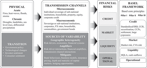
Transition risk drivers represent societal changes (such as progress toward affordability of existing technologies, alterations in public sector policies and investor/consumer sentiment towards a responsible, sustainable environment) which arise from the transition to a low-carbon economy. Although closely monitored by affected parties, these risk drivers could impact financial risks substantially because of their scale and synchronous deployment. Transition risks contribute to portfolio impacts such as value at risk (VaR) and tail—or extreme value—risk.

Transmission channels are the causal conduits through which climate risk drivers influence institutions (such as banks, corporates, and sovereigns) directly and indirectly through their assets, counterparties, and the local economy. The frequency and severity of climate risk driver impacts is influenced by several other variables including the geographic location of the corporate and correlations between transmission channels and climate risk drivers. The impact of climate risk drivers on corporates is manifest through traditional risk categories of credit, market, liquidity, and operational risk. Although the BCBS provides information regarding how climate risk drivers influence bank-specific financial risks, the framework is easily extended to all corporates (and other institutions) so the Basel Framework is included in Figure 1 to support the analysis in this article.

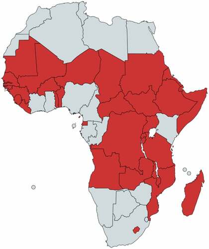
A joint report commissioned by the United Nations Environment Programme (UNEP) recently explored economic growth and development risks for African countries. Regions which will experience disproportionally higher risks from climate change (involving deteriorating health, reduced human and food security, altered water supply, and diminished economic growth) are developing island states and Least Developed Countries (UNCTAD, 2022)—of which 70% (32 out of 46) are African (IPCC, 2018) as shown in Figure 2. African countries will therefore be among the worst affected by rising temperatures impelled by climate change (indeed, any level of warming), with severe macroeconomic consequences impeding economic development.

Figure 2. African countries (shaded red) that will be severely affected by rising temperatures due to climate change. The remainder will also, inevitably, be impacted, but not as severely.

Source: Mapchart (2022) and author inputs.

Two climate change scenarios were considered: a low or optimistic scenario consistent with the goals established by the Paris Agreement (United Nations, 2015) in which global temperature rises are well below +2°C (at least until 2050) and a high-warming, pessimistic scenario which posits a global temperature increase of +2°C by 2050, and more than +4°C by 2100 (Baarsch & Schaeffer, 2019). Baarsch and Schaeffer (2019) argue that mitigating these impacts will require African Governments to integrate climate change risks into development and macroeconomic planning. At the microeconomic scale, assessing the impact of climate change on individual corporations’ credit risk and thus economic value, would contribute considerably to this integration.

Schlenker and Roberts (2009) developed and implemented a model for estimating the impacts of climate change on crop yields in the US. Bezabih et al. (2014) replicated and updated this approach to determine the effects of climate variability on Ethiopian crop production. Using these models, Baarsch and Schaeffer (2019) found that several African countries are already (2022) experiencing lower growth rates and diminished development due to climate change because of low adaptive capacities and limited resilience. GDP per capita growth is already lower in the poorest African countries, on average, by between 10% and 13% and projected macroeconomic consequences from climate change over the next three decades are severely detrimental. In a high-warming scenario, the GDP growth per capita of Eastern and Western African countries is forecast to fall below a baseline scenario (in which climate change does not affect macroeconomic development) by 15% by 2050. Northern and Southern Africa would also be considerably affected, with a 10% decrease in GDP growth by 2050. Central Africa would be less severely affected, with a decrease of 5% in a high-warming scenario (Baarsch & Schaeffer, 2019; Feyen et al., 2020).

By 2030 differences in macroeconomic costs between low and high-warming scenarios become apparent. By 2050, losses in high-warming scenarios are 50% higher for Central Africa and 85% higher for Western African regions. In optimistic (low-warming, low-emission, global) scenarios, however, i.e., those in line with the Paris Agreement’s aim of limiting global warming to below 2°C, simulations show that the most serious macroeconomic consequences for African countries can be circumvented (Feyen et al., 2020).

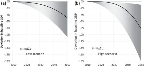
Climate-related disasters are expected to decelerate per capita African GDP growth, heaping pressure on sovereign budgets and fiscal balances, increasing government expenditure, reducing tax volumes, and ultimately swelling government debt. Figure 3 shows the GDP per capital deviation from a baseline over the next three decades for southern African countries resulting from simulations assuming two climate change scenarios.

Figure 3. GDP per capita deviation from a GDP per capita baseline scenario (in which climate change does not affect macroeconomic development) resulting from continued global warming for Southern African countries until 2050. (a) scenario in which global warming is below +2°C and (b) scenario in which global warming exceeds 2°C by 2050 and exceeds +4°C by 2100. Shaded regions represent a 68% statistical confidence interval (i.e., one standard deviation).

Source: authors’ calculations and Baarsch and Schaeffer (2019).

The remainder of this article proceeds as follows. Section 2 explores the relevant literature and contextualises the approach adopted in this article for credit assessment and assignment due to climate impacts. The data used for the analysis and simulations are described in Section 3 along with the mathematics governing the analytical approach adopted while Section 4 describes the output and results of the analysis, the consequences, and implications for affected corporates. Section 5 sets out the limitations of the study, presents possible future research and concludes.

2. Literature review

Empirical literature focussing on the impact of climate-related natural disasters (such as droughts and floods) on economic and social variables is somewhat limited. To bridge this gap in the literature, Shimada (2022) used an African regression model analysis with 50 years of panel data assembled over the period 1961–2011. Over this period, climate change-related natural disasters (principally droughts) negatively impacted Africa’s agriculture, economic growth, and poverty severely by affecting crops such as maize and coffee and increased the frequency and severity of armed conflicts (Shimada, 2022).

The BCBS (2021b) explored climate-related financial risk measurement methodologies, i.e., those risks of concern to banks and regulatory supervisors and distilled the work into key findings (BCBS, 2021a). Unique features of financial risks require forward-looking, granular measurement methodologies—necessarily involving forecasts based on sensible simulations. Banks and supervisors tend to focus on near term transition risk drivers with less progress made on bank exposures to physical risks and, to translate climate-related exposures to financial risk categories, banks’ have focussed on credit risk, less on market risk and even less on operational and liquidity risk. Modelling the impact of climate change on traditional credit risk parameters such as probabilities of default (PD) and losses given default (LGD) are in early stages and have yet to be standardised. Trial analyses have so far favoured a mix of approaches, including forward-looking methodologies and multiple scenario analysis, both involving forecasting of relevant variables, usually through simulations (BCBS, 2021).

Polbennikov et al. (2016) examined the relationship between historical environment, social and governance (ESG) ratings and US corporate bond spread and performance. Corporate bonds with high composite ESG ratings exhibited lower spreads and outperformed corporate bonds with low composite ESG ratings. Korean corporate bond data from 2010 to 2015 were used to explore the relationship between ESG scores and bond returns (Jang et al., 2020). The authors concluded that ESG scores embrace valuable information about the downside risk of firms, particularly for small corporates with high information asymmetry. Of the three ESG criteria, only environmental scores were found to impact bond returns significantly. ESG scores were also found to be complementary to credit ratings in assessing corporate credit quality. A similar study on stocks found that those with high ESG composite ratings generated higher realised returns and provided provide better tail-risk protection than stocks with low ESG composite ratings (Xiong, 2021). High ESG composite rated stocks provided considerable tail risk protection benefits during the COVID-19 crisis.

Using credit derivative prices, Thi Thu Truong and Kim (2019) explored the short- and long-run effects of ESG activities on implied credit risk. The authors used Fama-MacBeth regressions to show that firms with higher ESG scores exhibited lower credit risk (based on the analysis of associated credit default swaps) this is because, on average, ESG activities reduce credit risk in the long run more than in the short run.

The association between poor environmental performance and the combination of low-grade credit ratings and higher spreads for corporate bonds was demonstrated by Bauer and Hann (2010). Oikonomou et al. (2014) explored the link between environmental footprints and corporate debt by examining the impact of several sustainability performance dimensions on corporate debt pricing and specific bond issues’ credit quality. Adding corporate social responsibility factors lowered risk premia considerably, in turn reducing the corporate debt costs. Hoepner and Nilsson (2017) found that companies not embroiled in any environmental, social or governance issues (or scandals) outperform market benchmarks significantly regardless of maturity, particularly in times of market turmoil. Then authors conclude that investors price bonds on riskiness perceptions: companies fortunate to remain out of the news are thus perceived as less risky.

Capasso et al. (2020) explored the relationship between climate change and corporate credit risk using US data from 458 companies which issued investment grade fixed-rate corporate bonds over the decade from Dec-07 and Dec-17. A distance-to-default approach (a widely used market-based measure) for estimating default probabilities as a proxy for credit risk was used. This approach is derived from Black and Scholes (1973) and Merton’s (1974) work on option pricing which is employed here to price corporate debt. Capasso et al. (2020) established a clear link between exposure to climate risks and the creditworthiness of loans and bonds issued by corporates.

The European Banking Authority (EBA) recently (January 2022) published the final draft of Pillar III disclosures for the implementation of technical standards on ESG risks (EBA, 2022). These disclosures are designed, like all other Pillar III disclosures, to foster market discipline, and to allow stakeholders to assess banks’ ESG related risks and sustainable finance strategy. Banks must now disclose how climate change exacerbates their other balance sheet risks and how these are mitigated. In addition, banks’ must report their Green Asset Ratio (the ratio of the bank’s loans and securities meeting the EU environmental taxonomy to most on-balance sheet banking book assets). These disclosures are mandatory for all Basel-compliant banks from 1 January 2024.

In preparation for these new requirements, Licari et al. (2021) have developed a possible set of solutions which combined should enable institutions to assess risks posed by climate change. One aspect of the approach models the ongoing accumulation of carbon dioxide emissions and corresponding global temperature changes. These results are then fed into other model elements to ascertain physical and transition impacts of climate change on the relevant economy. Scenarios are flexible and can be adapted to require user inputs but Licari et al. (2021) explore scenarios consistent with those established by the Network of Central Banks and Supervisors for Greening the Financial System (namely Orderly, Disorderly, and Hot House World scenarios). The modelling framework is applied to two geographies, the US, and the UK, to establish reasonableness.

Edwards et al. (2021) extended the macroeconomic forecasting work of Licari et al. (2021) and adapted the approach for application to corporate credit. The methodology uses Moody’s Analytics Climate Adjusted expected default frequency (EDF) framework (explained in greater detail in Section 3). Although the augmented Moody’s EDF approach for climate risk comprises several connected components, the physical risk-adjusted EDF and the transition risk-adjusted EDF modules are of particular interest.

3. Data and methodology

3.1. Data

Unlike Capasso et al. (2020) who used real corporate data over a specified historical period (companies were selected on the basis that they had issued investment grade debt during this period), we used simulated data for all our analysis. Studies such as those by Castro et al. (2021) which investigate the impact of severe environmental changes on stock prices, are rare but increasing (see, e.g., Faccini et al., 2022 and sources therein). Because of this dearth of data linking climate-related impacts on share prices, we simulate these results for a range of possible impacts. Affected firms may use their own judgment regarding the nature (physical or transition) and scale of any relevant climate-related impacts: we provide a theoretical (and practical) approach for establishing a calibration for such impacts.

To determine the evolution over time of corporate asset and liability values, we used a GBM approach with a range of stylistic annual volatility and drift values on ten years of weekly share prices. Shocks were introduced at different times with varying severity (in percentage terms). Again, the frequency and severity of such shocks may be decided upon by individual affected firms and then implemented.

Outputs from the GBM analysis become inputs for the KMV model (like Baarsch and Schaeffer’s (2019) approach), and here again, simulated (but realistic) parameters for equity volatility, liabilities, market value of assets, risk-free rates, etc., are used. Firms may use their own values for these parameters or obtain such from publicly sourced balance sheets and other corporate data.

3.2. Methodology

The primary aim is to assess the impact of climate transition and physical risk on obligor creditworthiness. This evaluation could be translated into a measure of default probability, which may then be used for IFRS-9 accounting reporting, regulatory credit risk measurements, forecasting and other relevant and important information of affected firms.

The approach involves simulating asset values over time (using GBM) and then stress testing these asset values by introducing a climate event. If the event is “physical”, the shock is immediate, unexpected, and the ramifications can be of varying severity and duration. An important distinction between physical and transition climate shocks is that physical shocks cause the underlying asset volatility to increase after the event while for transition shocks asset volatilities do not increase because the event (such as a policy change or a new sustainable tax) was anticipated.

3.2.1. Geometric Brownian motion

We assume that stock price returns are lognormally distributed, i.e., we assume that asset values, $S$, evolve according to a lognormal distribution over time (Agustini et al., 2018), i.e., that

$ln\left(\frac{S_t}{S_0}\right)\sim \varphi \left[\left(\mu -\frac{{\sigma }^2}{2}\right)dt,\sigma \sqrt{dt}\right]$

which implies that

$dS=S_{t}exp\left[\left(\mu -\frac{{\sigma }^2}{2}\right)dt+\sigma \epsilon \sqrt{dt}\right]$

where $S_t$ represents the stock price at time $t$, $dt$ is the time over which the return is measured, $\mu$ is the average return, ${\sigma }^2$ is the return variance, the term in round brackets represents the stock price drift over time, and $\epsilon$ is distributed $\sim N\left(0,1\right)$. In discrete terms (i.e., where the continuous time variable $dt$ is replaced by the discrete time step $\mathrm{\Delta }t$)

$S_{dt+\mathrm{\Delta }t}=S_{t}exp\left[\left(\mu -\frac{{\sigma }^2}{2}\right)\mathrm{\Delta }t+\sigma \epsilon \sqrt{\mathrm{\Delta }t}\right]$

The time step is commonly taken to be $t=1$ day for most stock price simulations, although $t$ can be any sensible time unit, and which may be adjusted to fit the specific forecast problem. In this work, because annual default rates are the product, daily simulations were deemed too granular while monthly and annual simulation steps led to considerably reduced scenario numbers and diminished forecast accuracy. As a result, weekly timesteps were used to provide some output granularity without sacrificing model accuracy.

Ten years of weekly simulations were generated. This provided enough forecast scenarios to make reasoned observations on ESG event impact severity and duration. By arranging the event to occur—say—in one year’s time and allowing the event’s impact to affect the asset value in accordance with the KMV model predictions, the propagation of the impact could be monitored and assessed over the next nine years. While longer obligation periods exist, this period is sufficient to identify patterns and features in default rates (and other outputs such as post-event volatility) and isolate the effects of event severity and duration. We also explored the impact of multiple climate-related impacts, of different severities, to assess the effect of such events.

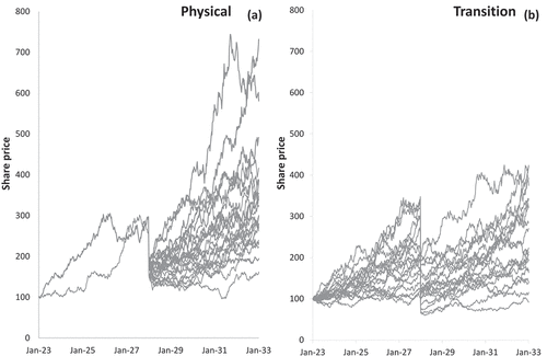
We generated 10000 stock price simulations, all with the arbitrarily selected start value of 100 but we reproduce only a few paths for clarity in Figure 4. Share price ($y$) axes scales are the same for both types of events for comparison.

Figure 4. Simulated share prices for a 60% share price shock occurring halfway through a ten-year simulation cycle, due to (a) a physical climate risk event in which volatilities post the even do increase by 10% and (b) a transition climate risk event in which equity volatilities do not increase after the event. Note the same vertical scale for comparison.

Source: Author’s calculations.

3.2.2. KMV PD estimation

Crosbie and Bohn (2003) set out the mathematics governing the estimation of default probabilities from equity prices. Assume

(1) $d{V}_A=\mu V_{A}dt+{\sigma }_A{V}_{A}dz$(1)

where $V_A$ and $d{V}_A$ are the firm’s asset value and change in asset value, $\mu$ and ${\sigma }_A$ are the firm’s asset value drift rate and volatility, and $dz$ is a Wiener process.

The KMV model allows only two types of liabilities, a single class of debt ($X$) and a single class of equity. If $X$ is the book value of the debt due at time $T$ then the market value of equity and the market value of assets, respectively, are related using:

(2) $V_E=V_{A}N\left(d_1\right)-exp\left(rT\right)XN\left(d_2\right)$(2)

where $V_E$ is the market value of the firm’s equity, $r$ is the risk-free interest rate and

$d_1=\frac{ln\left(\frac{V_A}{X}\right)+\left(r-\frac{{\sigma }_A^2}{2}\right)T}{{\sigma }_A\sqrt{T}}$

$d_2=d_1-{\sigma }_A\sqrt{T},$

A firm’s equity volatility is then related to its asset volatility using

(3) ${\sigma }_E=\frac{V_A}{V_E}\mathrm{\Delta }{\sigma }_A$(3)

Asset values and volatilities implied by equity values, volatilities and liabilities are determined by solving the call price (2) and volatility (3) equations, simultaneously.

The probability of such a firm defaulting is the probability that the firm’s asset market value will be less than the firm’s liabilities book value when the debt matures. This may be written

(4) $p_t=Pr\left[V_A^t\le X_t|V_A^0=V_A\right]=Pr\left[ln{V}_A^t\le ln{X}_t|V_A^0=V_A\right]$(4)

where $p_t$ is the probability of default by time $t$, $V_A^t$ is the market value of the firm’s assets at time $t$, and $X_t$ is the book value of the firm’s liabilities due at time $t$. The change in the value of the firm’s assets is described by (1) and thus the value at time $t$, $V_A^t$, given that the value at time $0$ is $V_A$, is:

(5) $ln\left(\frac{V_A^t}{V_A^0}\right)=\left(\mu -\frac{{\sigma }_A^2}{2}\right)t+{\sigma }_A\epsilon \sqrt{t}$(5)

where $\mu$ is the expected return on the firm’s asset, and $\epsilon$ is the random component of the firm’s return. This is the evolution of the asset value. Combining (4) and (5) gives the probability of default becomes:

$p_t=Pr\left[ln{V}_A+\left(\mu -\frac{{\sigma }_A^2}{2}\right)t+{\sigma }_A\epsilon \sqrt{t}\le X_t\right]$

which may be rearranged to give

$p_t=Pr-\frac{ln\left(\frac{V_A}{X_t}\right)+\left(\mu -\frac{{\sigma }_A^2}{2}\right)t}{{\sigma }_A\sqrt{t}}\le \epsilon$

Recall that the Black and Scholes model assumes that the random component of the firm’s asset returns is normally distributed, $\epsilon \sim N\left(0,1\right)$ as a result the default probability may be defined in terms of the cumulative Normal distribution:

$p_t=N\left[-\frac{ln\left(\frac{V_A}{X_t}\right)+\left(\mu -\frac{{\sigma }_A^2}{2}\right)t}{{\sigma }_A\sqrt{t}}\right]$

The distance-to-default is the number of standard deviations that the firm is away from default and thus in the Black and Scholes formulation is:

(6) $DD=\frac{ln\left(\frac{V_A}{X_t}\right)+\left(\mu -\frac{{\sigma }_A^2}{2}\right)t}{{\sigma }_A\sqrt{t}}$(6)

The approach, then, is:

1. simulate share prices using realistic parameter inputs, such as drift and equity return volatility

2. introduce realistic climate-induced shocks of different frequencies and severities

3. record resulting average firm market values (via share prices) and equity volatilities at selected time intervals after the introduction of the shock(s)

4. input these asset values and equity volatilities into the KMV model to estimate the DD (6) and hence the change from unshocked DDs

5. set up a calibration scale for different climate shocks (physical or transition), shock severities and impact on underlying credit quality.

Steps (1–5) provide a way to calibrate the impact of shock size on corporate default rates.

4. Results and discussion

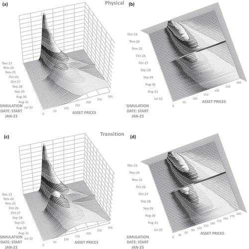
The GBM approach was used to simulate10000potential equity price scenarios, weekly, over ten years. Figure 5 shows a 3D view of the results of these simulations. At each timestep, the mean and standard deviation of the distribution of possible share prices are used to plot the log normal distribution of outcomes. A shock (in this example a $-40\mathrm{\%}$ share price shock) is then introduced at time $t$ (in this example halfway through the 10-year simulation on 1 January 2028). Prices after physical shocks have increased volatilities while those for transition shocks do not.

Figure 5. Simulated lognormal distributions (side and plan view) of share prices for a 40% share price shock occurring halfway through a ten-year simulation cycle, due to (a) a physical climate risk event and (b) a transition climate risk event.

Source: Author’s calculations.

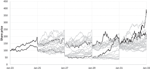
Scenarios involving several shocks were also investigated. In Figure 6, these were introduced at two-year intervals since the start (1 January 2023) of the simulations, but frequencies and severities can be altered to suit practitioner expectations.

Figure 6. Simulated share prices for 40% share price shocks occurring at two-year intervals through a ten-year simulation cycle, due to physical climate risk events.

Source: Author’s calculations.

Outputs (average share prices and equity volatilities) were then used to assess DDs using the KMV model and (6) for various shock severities, shock frequencies and applied to different credit grades. A 40% equity price shock, for example, is expected to have a considerably greater impact on a CCC-rated (high PD) credit than on a AAA-rated (low PD) credit. This turns out to be the case, with average uncertainty ranges being roughly equal as shown in Figure 7. For the results shown in Figure 7, PDs averaged over the period 1920–2020 from associated credit ratings were sourced from S&P Global Ratings (2021).

Figure 7. Scaling factor increase in PD for $-20\%$, $-40\%$, $-60\%$ and $-80\%$ equity price shocks for (a) a physical climate event for credit grades AAA through BBB, (b) a physical climate event for credit grades BBB- through CCC/C, (c) a transition climate event for credit grades AAA through BBB and (d) a transition climate event for credit grades BBB- through CCC/C.

Source: Authors’ calculations.

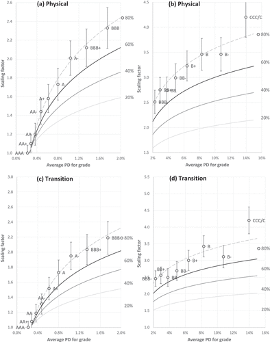
Increases in PDs for highly rated credit are negligible, but increase in severity up to $\approx 4$ for poorest rated credits. Climate change impacts on PDs are non-negligible and can be severe.

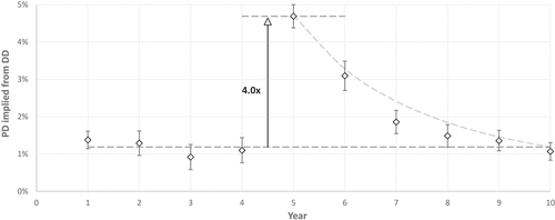
Figure 8 shows the time decay of a 60% climate change shock on the implied PD of an A- credit with average unshocked PD of $\sim 1\mathrm{\%}$ (derived from DDs). The shock introduces a steep fourfold increase in PD, and if there are no subsequent shocks, the PD recovers, ceteris paribus, roughly exponentially to former PD levels within five years. This is by design a stylistic example, subject to the user’s inputs and opinions on volatilities, and both the frequency and the severity of the applied shocks, but it does give some indication of how PDs may change with climate-related events.

Figure 8. Time decay of a 60% climate change shock on the implied PD of an A- credit.

Source: Author’s calculations.

If multiple climate-event shocks—even of mild (20%) severity—are administered at a frequency of one year or less, the firm invariable defaults. The share price is unable to recover no matter the price drift or post-shock equity volatility and the firm defaults. This scenario speaks to consequences for a future in which climate related shocks arrive with increasing frequency, regardless of the shock’s severity.

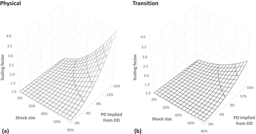
The outcome of the analysis is shown in Figure 9. The scaling factor, which should be applied to unshocked PDs ($z$-axis) has been plotted as a function of shock size and original PD to which the climate-related shock has been applied. As expected, the scaling factor increases as a function of both parameters (shock severity and original, unshocked PD) for both physical and transition climate events. Such a calibration can be applied to a firm’s obligors to assess forward looking PDs, dependent on climate shocks.

Figure 9. Scaling factor to be applied to unshocked obligor PDs for (a) physical and (b) transition related climate events as a function of shock size and unshocked PD. Again, note the same vertical scale for comparison.

Source: Author’s calculations.

5. Conclusion and recommendations

Climate related impacts—whether of physical or transitional origin—have been quantified, calibrated, and used to assess credit quality degradation. The inputs are by nature subjective and must be determined by the user; obligors have unique share price drifts and volatilities, and shock scenarios vary by type, severity, and frequency. This provides considerable flexibility, however. As more climate related events are added to the literature and global databases, specific climate events will eventually be linked to specific shock sizes (so floods might result in a physical shock of 32% while a policy announcement of a carbon tax increase might result in a transition shock of 18%, and so on). The approach outlined in this article should then become less subjective as only the event type will need to be identified.

These results will be of considerable benefit to all IFRS-9 compliant market participants (for forward looking scenarios of obligor credit quality) but also for loan pricing which uses obligor PDs and regulatory capital calculations (which require knowledge of PDs at multiple maturities, not just one-year).

Limitations include the usual limitations argued against the KMV model, namely that the model requires subjective estimation of some input parameters, it assumes that asset returns are normally distributed, it does not distinguish between bonds of different seniority, collateral, covenants, or convertibility and private (unlisted) firms’ expected default frequencies may be calculated only by applying some comparability analysis, usually derived from accounting information. In addition, until some objective database can be installed which isolates the relevant impact frequency and severity of different climate-related events, these inputs will remain in the domain of subject matter experts or experienced economists. Either way, they will be subjective, so some degree of caution should be applied and error bars reflecting the inherent uncertainty associated with this analysis, should be observed.

Possible future work could include mapping specific climate events to credit quality degradation as more data become available. The authors concur that some time may elapse before substantial databases documenting these linkages become available, commonplace and widely used.

Table

List of acronyms
BCBS	– Basel Committee on Banking Supervision
EAD	– exposure at default
EBA	– European Banking Authority
EDF	– expected default frequency
EL	– expected losses
ESG	– environmental, social, governance
GBM	– geometric Brownian motion
GDP	– gross domestic product
IPCC	– Intergovernmental Panel on Climate Change
KMV	– Kolmogorov Merton Vasicek
LGD	– loss given default
PD	– probability of default
UL	– unexpected losses
UNCTAD	– United Nations Conference on Trade and Development
UNEP	– United Nations Environment Programme
VaR	– Value at Risk

Ethics statement

No animal or human studies involved – all data are non-proprietary and freely available from the internet and other non-proprietary sources

Disclosure statement

No potential conflict of interest was reported by the author(s).

Additional information

Funding

The authors received no direct funding for this research.

Notes on contributors

Francesca Bell

Francesca Bell – completed her undergraduate and Honours degrees at the University of Cape Town, specialising in investment management and portfolio analysis. Now wrapping up her Masters degree covering the interrelatedness of modern finance and ESG factors at the University of the Witwatersrand, she also works as a quantitative research analyst at RiskWorx, a boutique consulting firm in Sandton, Johannesburg. ESG-related issues continue to dominate the news and the social conscience of informed citizens. Corporate probabilities of default – and credit risk in general – can be significantly influenced by environmental factors: sensible research is sorely needed to establish how this interaction operates, how the type and magnitude of climate events affect credit riskiness and how these effects may be measured and mitigated.

Gary van Vuuren

Gary van Vuuren – is a professor at the University of the Witwatersrand, where he supervises postgraduate research in risk measurement and management.

References

- Agustini, F., Restu, W. I., Endah, A., & Putri, R. M. 2018. Stock price prediction using geometric Brownian motion. Journal of Physics Conference Series, 974, 12047: 1–16.
- Ahmad, N., Mobarek, A., Roni, N. N., & Tan, A. W. K. (2021). Revisiting the impact of ESG on financial performance of FTSE350 UK firms: Static and dynamic panel data analysis. Cogent Business & Management, 8(1), 1–18. https://doi.org/10.1080/23311975.2021.1900500
- Baarsch, F., & Schaeffer, M. 2019. Climate change impacts on Africa’s economic growth. United Nations Economic Commission for Africa report, African Development Bank Group. Available from: https://www.afdb.org/sites/default/files/documents/publications/afdb-economics_of_climate_change_in_africa.pdf, accessed 13 Feb 22
- Bauer, R., & Hann, D. 2010. Corporate environmental management and credit risk. Maastricht University. 1–44. https://doi.org/10.2139/ssrn.1660470
- BCBS., 2021a. Climate-related risk drivers and their transmission channels. Available from: https://www.bis.org/bcbs/publ/d517.pdf, accessed 17 Apr 22
- BCBS., 2021b. Climate-related financial risks – Measurement methodologies. Available from: https://www.bis.org/bcbs/publ/d518.pdf, accessed 16 Apr 22
- Bezabih, M., Di Falco, S., & Mekonnen, A. 2014. Is it the climate or the weather? Differential economic impacts of climatic factors in Ethiopia. Centre for Climate Change, Economics and Policy, working paper #148. https://www.lse.ac.uk/GranthamInstitute/wp-content/uploads/2014/02/WP148-Is-it-the-climate-or-the-weather-impacts-on-climatic-factors-in-Ethiopia.pdf
- Black, F., & Scholes, M. (1973). the pricing of options and corporate liabilities. Journal of Political Economy, 81(3), 637–654. https://doi.org/10.1086/260062
- Capasso, G., Gianfrate, G., & Spinelli, M. (2020). Climate change and credit risk. Journal of Cleaner Production, 266(1), 1–10. https://doi.org/10.1016/j.jclepro.2020.121634
- Castro, P., Gutierrez-Lopez, C., Tascon, M. T., & Castano, F. J. (2021). The impact of environmental performance on stock prices in the green and innovative context. Journal of Cleaner Production, 320(5), 1–12. https://doi.org/10.1016/j.jclepro.2021.128868
- Crosbie, P., & Bohn, J. 2003. Modeling default risk. KMV internal report. Available from: https://www.moodysanalytics.com/-/media/whitepaper/before-2011/12-18-03-modeling-default-risk.pdf, accessed 5 Mar 22.
- EBA., 2022. Final draft implementing technical standards on prudential disclosures on ESG risks in accordance with Article 449a CRR. Available from https://www.eba.europa.eu/eba-publishes-binding-standards-pillar-3-disclosures-esg-risks, accessed 16 Apr 22
- Edwards, J., Cui, R., & Mukherjee, A. 2021. Assessing the credit impact of climate risk for corporates. Moody’s Analytics. Available from: https://www.moodysanalytics.com/-/media/whitepaper/2021/assessing-the-credit-impact-of-climate-risk-for-corporates.pdf, accessed 7 Jan 22.
- Faccini, R., Rastin, M., & Skiadopoulos, G. S. 2022. Dissecting climate risks: Are they reflected in stock prices? https://ssrn.com/abstract=3795964
- Feyen, E., Utz, R., Huertas, I. Z., Bodgan, O., & Moon, J. 2020. Macro-financial aspects of climate change. World Bank Policy Research, working Paper #9109.
- Hoepner, A., & Nilsson, M. 2017. No news is good news: Corporate social responsibility ratings and fixed income portfolios. SSRN Electronic Journal https://ssrn.com/abstract=2943583
- IPCC., 2018. Intergovernmental panel on climate change special report: Global warming of 1.5°C. Available from: https://www.ipcc.ch/sr15/, accessed 16 Apr 22
- Jang, G., Kang, H., Lee, J., & Bae, K. (2020). ESG scores and the credit market. Sustainability, 12(8), 3456–3476. https://doi.org/10.3390/su12083456
- Licari, J., Zemcik, P., Lafakis, C., & Lee, J. 2021. Climate risk macroeconomic forecasting. Moody’s Analytics. Available from: https://www.moodysanalytics.com/-/media/article/2021/Climate-Risk-Scenarios-Modeling.pdf, accessed 2 Jan 22
- Mapchart. 2022. Available from https://www.mapchart.net/africa.html, accessed 17 Apr 22
- Merton, R. C. (1974). On the pricing of corporate debt: The risk structure of interest rates. Journal of Finance, 29(2), 449–470. https://doi.org/10.1111/j.1540-6261.1974.tb03058.x
- Oikonomou, I., Brooks, C., & Pavelin, S. (2014). The effects of corporate social performance on the cost of corporate debt and credit ratings. The Financial Review, 49(3), 49–75. https://doi.org/10.1111/fire.12025
- Polbennikov, S., Desclée, A., Dynkin, L., & Maitra, A. (2016). ESG ratings and performance of corporate bonds. The Journal of Fixed Income, 26(1), 21–41. https://doi.org/10.3905/jfi.2016.26.1.021
- Schlenker, W., & Roberts, M. J. 2009. Nonlinear temperature effects indicate severe damages to US crop yields under climate change. Proceedings of the National Academy of Sciences of the United States of America, 106(37): 15 594–15 598.
- Shimada, G. (2022). The impact of climate-change-related disasters on Africa’s economic growth, agriculture, and conflicts: Can humanitarian aid and food assistance offset the damage? International Journal of Environmental Research and Public Health, 19(1), 1–16. https://doi.org/10.3390/ijerph19010467
- S&P Global Ratings., 2021. Default, transition, and recovery: 2020 annual global corporate default and rating transition study. Available from https://www.spglobal.com/ratings/en/research/articles/210407-default-transition-and-recovery-2020-annual-global-corporate-default-and-rating-transition-study-11900573
- Thi Thu Truong, T., & Kim, J. (2019). Do corporate social responsibility activities reduce credit risk? Short and long-term perspectives. Sustainability, 11(24), 696–716. https://doi.org/10.3390/su11246962
- UNCTAD., 2022. UN list of least developed countries. Available from: https://unctad.org/topic/least-developed-countries/list, accessed 16 Apr 22
- United Nations., 2015. The Paris agreement. Available from: https://www.un.org/en/climatechange/paris-agreement, accessed 16 Apr 22
- Xiong, J. X. (2021). The impact of ESG risk on stocks. The Journal of Impact and ESG Investing, 2(1), 7–18. https://doi.org/10.3905/jesg.2021.1.025