Employing a generalized reduced gradient algorithm method to form combinations of steel price forecasts generated separately by ARIMA-TF and ANN models

Abstract

The research objective of the present study is the development of a model for increased accuracy of steel-price forecasts, which is of paramount importance for firms who use steel as an input and thus need to make informed decisions with regard to an optimal amount and type of hedge against unfavourable steel-price movement. To achieve its aim, the study forms weighted average combinations of steel price forecasts generated separately by a transfer function ARIMA model (ARIMA-TF) and an artificial neural network model (ANN), as both models are shown to contribute independent information with regard to target variable (steel price) movement. A generalized reduced gradient algorithm (GRG) method is employed to estimate the component model forecast weights, which is a novel approach introduced by this study. The data set employed includes a time series of monthly steel prices (cold rolled flat steel) from February, 2012 to November, 2020. Explanatory variables include iron ore price, coking coal price, capacity utilization, GDP and industrial production. With regard to the out of sample forecasts of all models (component and combining), mean absolute percentage forecast errors (MAPE) are calculated and model comparisons are made. The study finds that the combining model formed with the gradient algorithm approach in which the weights are constrained to be nonnegative and sum to one has the lowest MAPE of all models tested, and overall is found to be very competitive with other models tested in the study. The policy implication for firms that use steel as a major input is to base their hedging decisions on a combination of forecasts generated by ARIMA-TF and ANN models, with the forecast weights generated by a constrained generalized reduced gradient algorithm (GRG) method.

Keywords:

• steel price forecasts
• ARIMA transfer function
• Artificial Neural Network (ANN)
• Gradient Algorithm constrained optimization
• Constrained weighted least squares (WLS) regression analysis
• combination forecasting

JEL code:

• C53 Forecasting and Prediction Methods
• Simulation Methods

1. Introduction

The central aim of this study is to implement constrained optimization methods in forming an optimal combining model, with regard to steel-price forecasts. The component forecasting models employed are a transfer function ARIMA (ARIMA-TF) model, and an artificial neural network (ANN) model. The research problem that this paper addresses is increased accuracy of steel-price forecasts. There is one obvious group for whom forecast accuracy of steel prices is critical: Firms who use steel as an input and thus need to make informed decisions with regard to hedging against unfavorable steel-price movement, either with futures or options contracts; and/or by steel-input inventory stockpiling. In a survey of large U.S. nonfinancial firms, Bodnar et al. (1995) find that about 40% (of respondents) use derivatives to hedge against operating risk, including commodity-input price risk. In a more recent paper, Ajupov et al. (2015) indicate that hedging with derivatives appears to be the most common or preferred strategy in the automotive sector (for whom steel is a major input); and could involve the purchase of call options contracts, or the purchase of a forward contract; depending in part on bullish or bearish forecasts of steel input prices. Derivative hedging may be preferable to steel-input stock piling, for a number of reasons. For example, if demand were to drop off for such steel-products as cars or consumer durables, manufacturers could be saddled with excess steel-input inventory. Additionally, input stock piling could exacerbate the problem with the resultant artificial demand fueling greater steel input prices (Mathews, 2011). There is also the issue of the cost of stock piling to consider, including the construction and maintenance of warehouses. However, for firms such as auto makers that typically use a just in time production system (in which costs are controlled by keeping excess input supply to a minimum), a cut-off from a steel supplier based on a contract dispute over increased steel prices could significantly interrupt production operations (Hakim, 2003). Such firms are likely to consider at least a partial hedge with inventory stock piling. Turcic, (2014) address the issue of such non-cooperative behavior in a supply chain in which manufacturers purchase steel from suppliers that buy steel directly from steelmakers, and then process that steel (stamp, bend, coat and cut) for auto and consumer durable makers. They provide a rationale and offer strategies for hedging with derivatives for manufacturing firms using steel as an input, and operating in such a supply chain. Clearly, accuracy of steel-price forecasts is paramount for firms who utilize use steel as an input, with regard to the firm’s decision of the optimal amount and type of hedge.

This paper undertakes the research problem of developing a model with the objective of improved steel-price forecast accuracy. It stands to reason that the greater the information set on which price-forecasts are based, the greater the potential for enhanced forecast accuracy (Liu, 2020). One established method to achieve a greater information set is to form combinations of forecasts generated by two or more different component models that each contribute independent-information content, with regard to target-variable movement (Bates & Granger, 1969; Bischoff, 1989; Fair & Shiller, 1990). Additionally, combining forecasts of different forecasting models may capture different aspects of the information set available for prediction, without having to identify the underlying process behind a singular model forecast (Clemen, 1989). One or more models may contribute independent-information by either employing different data, or by processing the same data differently (Bates & Granger, 1969). Each of the two component models in the present study (ARIMA-TF and ANN) employs a different data set; and each model processes a common data set differently. Thus each model is likely to contribute independent information with regard to movement of the steel price forecast variable; which makes both models suitable candidates in forming a combining model. Specifically, with regard to processing same data differently, an ARIMA model can be used to analyze any linear functional relations inherent in the data, but not nonlinear; whilst an ANN model does have nonlinear modelling capability, adaptively formed based on any functional relations inherent in the data (Zhang, 2003; Kim et al., 2022). However, as Zhang points out, in practice there may be difficulty in ascertaining whether a particular time-series is generated from a linear or nonlinear underlying set of functional relations; or in fact may be inclusive of both linear and nonlinear functional relations. Echoing the above assertion stated by Clemen (1989), both the Zhang and Kim et al. studies suggest that one way to overcome these issues is to model linear and nonlinear functional relations separately with an employment of ARIMA and ANN models, respectively; and then form a combination of the component model forecasts. In this way, a combining method is able harness both the ARIMA and ANN models in discerning different functional relations inherent in the data, thereby leading to a provision of independent information content by each model. And in fact, in the present study, a test of independent information with an in sample regression analysis (Cooper & Nelson, 1975; Fair & Shiller, 1990; Nelson, 1972) finds the existence of an independent information content in the component model forecasts (ARIMA and ANN) to be the case. As Kim et al., (2022) note, an additional benefit in forming a combination of ARIMA and ANN forecasts lies in utilizing the distinctive strengths of each model to alleviate the limitations of each model: The inclusion of an ARIMA model forecast in the combining model can mitigate the overfitting problems of the ANN; while the inclusion of the ANN forecast can capture the nonlinear dynamics of the time series that the that the ARIMA model is unable to. As a result, the combining model can reduce the forecasting errors stemming from both the overfitting problems of the ANN and the inability of the ARIMA model to capture nonlinear functions in the time series.

With regard to forming a combining model, both the Zhang (2003) and Kim et al., (2022) studies successfully experiment with a two-stage hybrid method, in which an ARIMA model is used to analyze any linear functional relation inherent in the data; and an ANN model is developed to model the residuals from the ARIMA model, which will contain information about any nonlinear functional relations. Both studies find that the resultant combining model consistently outperforms both ARIMA and ANN models, in terms of lower forecast error.The present study takes a different approach in forming a combining model, with the utilization of two different constrained optimization methods: (1) A novel approach in which a generalized reduced gradient algorithm [GRG] technique (L. L. Lasdon et al., 1974; L. S. L. S. Lasdon et al., 1978) is employed to estimate the component model forecast weights. GRG algorithm maximizes or minimizes an objective function with respect to given constraints (such as constraining the combining model forecast weights to be nonnegative and sum to one); which makes GRG algorithm perfectly suitable for error minimization optimizations, including the estimation of combination forecast weights such that forecast error is minimized. (2) A combining model is also formed with the more conventional approach of using estimated regression [in sample] coefficients as forecast weights for the combining model [out of sample]. Pioneers of this latter approach include Nelson (1972), Cooper and Nelson (1975), and Fair and Shiller (1990), who each employed ordinary least squares (OLS) regressions [in sample] of realized values of the target variable against predicted values made by component models, to generate the weights for the combining model [out of sample]. (The method of weighted least squares [WLS] regression analysis is utilized instead of OLS in the present analysis to overcome the problem of heteroscedasticity.) One advantage to using the GRG method to estimate the forecast weights for the combining model is the flexibility to minimize any selected error statistic; whilst the WLS approach is limited to minimizing sum of squared error (SSE), like all other regression-based approaches.

There are two aspects of the research gap that the present study addresses: One, there is a dearth of studies in which the method of combination forecasting is employed to forecast steel-prices. In fact, the present analysis appears to be the initial study to do so. Second, the method of using a generalized reduced gradient algorithm (GRG) technique to estimate the component model forecast weights appears to be a novel approach that is being introduced in this study.

Using only data available prior to an out of sample forecast horizon, the present study generates simulated, ex ante out of sample component model forecasts (ARIMA-TF and ANN) and combining model forecasts of steel prices (employing in turn both the WLS and GRG methods of generating component forecast weights for the combining model). In terms of forecast accuracy as measured by mean absolute percentage error (MAPE), the study finds that both combining model techniques (WLS and GRG) outperform both component models (ARIMA-TF) and ANN); and the combining model formed with the generalized reduced gradient algorithm (GRG) technique outperforms the combining model formed with WLS estimated regression coefficients. However, the results are mixed (to some extent) when another measure of forecast accuracy is considered (root mean square error [RMSE]); and when the differences in forecast error between two models are tested for statistical significance. These findings are discussed in more detail below, in section 4.

The paper is organized as follows: Following the section 1 introduction above, section 2 presents a review of relevant studies to provide context, further indicate research gaps and provide a broader, deeper and more detailed theoretical foundation from which the empirical analysis emanates. Section 3 indicates the data and presents the different methodologies employed in the analysis to generate the different models’ forecasts and to test the results. Section 4 presents and discusses the empirical findings. The paper concludes with summary remarks and conclusions in Section 5.

2. Background

2.1. Steel-price forecasting

With regard to steel price forecasting, there appears to be a research gap in the form of a dearth of studies that endeavour to improve forecast accuracy by combining forecasts of different models. In fact, the present study appears to be the initial attempt. Instead, researchers have tended to employ a singular-model approach, over a range of forecast models of three main types: Multiple regression functions; time-series models; and multivariate Artificial Neural Network (ANN) models.

For example, Mancke (1968), Liebman (2006), Yuzefovych (2006), and Malanichev and Vorobyev (2011) each forecast steel prices with a multiple regression function, with variety of explanatory variables. The factors of demand, supply and market structure are found to significantly affect steel prices in the model employed by Mancke. Safeguard tariffs and antidumping duties, along with other variables (including industrial production; ore price; coal price) are found to have a significant impact on US steel prices in the Liebman study. In a simultaneous equation system for steel price and demand of Eastern Europe (EU), the Yuzefovych study finds that explanatory variables in the form of production indices of US, EU and China are significantly related to steel price. Among explanatory variables including time and raw material price (a weighted average of iron ore and coking coal prices), capacity utilization is found to be the major determinant of steel price in the Malanichev and Vorobyev study.

Chou (2013), Kapl and Müller (2010), and Adli and Sener (2021) each experiment with a different form of time-series modelling to forecast steel prices. Chou employed a fuzzy time series model for long term forecasting of an annual global steel price index, and presented results with a 4.4% mean absolute percentage forecast error (MAPE). Kapl and Muller forecasted quarterly steel price series with a multi-channel singular spectrum analysis (MSSA) and ARIMA models. Both types of time-series models presented similar forecasting precision, according to their results. Adli and Sener (2021) forecasted U.S. steel prices with vector auto regression in levels (LVAR) and vector error correction (VEC) models. Their findings indicate that whilst LVAR produces successful results for short term forecasting, the VEC model can relied upon for both short- and long-term forecasting. The LVAR model produced the greatest forecast accuracy in their research.

Liu et al. (2015) and Mir et al. (2021) each employ a multivariate Artificial Neural Network (ANN) model to forecast steel prices. Using explanatory variables including an iron ore price index, a rebar [reinforcement steel bars] price index and a rebar trading volume, the Liu et al. study forecasts a Chinese steel price index with a 6.8% MAPE. In the Mir et al. study, the most significant variables affecting steel prices in their multivariate ANN model are an iron ore price index, a consumer price index and housing starts.

The current study, then, attempts to fill this research gap and contribute to the literature with regard to steel-price forecasting, by forming a combining model in which forecasts generated independently by a transfer function ARIMA model (ARIMA-TF) and a multivariate Artificial Neural Network (ANN) model are formed into a weighted average; with the component model forecast weights estimated alternately by a generalized reduced gradient algorithm (GRG) method, and by a weighted least squares (WLS) regression analysis.

2.2. Combination forecasting

The concept of combination forecasting appears to have originated with Bates and Granger (1969). The underlying theory introduced in their study is that improved forecast accuracy may be achieved by combining forecasts of two (or more) component models, given that each provides independent information regarding the sources of movement of the forecast variable. The Bischoff (1989) combination forecast study provides an investment portfolio approach analogy to help explain this combining model theory: A portfolio composed of two or more securities may have a lower variance than any individual security if the returns from the securities are not perfectly correlated. Likewise, combining individual forecasts that embody different, independent information may lead to a composite forecast superior to either individual forecast. Put another way, as noted by Rapach and Strauss (2009), much like diversification across individual assets reduces a portfolio’s variance, combining singular model forecasts lowers the forecast variance relative to any of the individual predictive model forecasts. In other words, forecasts can always be combined in such a way that the composite forecast has variance less than or equal to any of the competing forecasts (Diebold & Pauly, 1987). As Bischoff (1989) notes, Nelson (1972) and C. Granger and Newbold (1975) find that combination forecasts have smaller root-mean-square-errors than the individual component model forecasts. As put forth by Bates and Granger (1969)1969, two or more models may contribute independent-information content by either employing different data, or by processing the same data differently. Testing for the existence of independent-information content in two or more candidate models can be achieved with a regression analysis in which realized values of the target variable are regressed against in-sample forecasts made by the two (or more) different component models (Bischoff, 1989; Cooper & Nelson, 1975; Nelson, 1972). If the estimated regression coefficients are nonzero and separately identified, then the existence of independent-information content is confirmed; and forming combinations of those respective component models’ forecasts may achieve superior forecast accuracy (C. Bischoff, 1989; Fair & Shiller, 1990; C. Granger & Newbold, 1975). In addition to testing for the existence of independent information, the estimated in-sample regression coefficients serve another purpose. The coefficients, if found to be nonzero and separately identified, give indication as to the appropriate proportional values of the weights to assign to each component forecast in the out-of-sample combination model (Nelson, 1972); Cooper and Nelson (1975); Fair & Shiller, 1990).

There have been other different approaches with regard to combining methods with varying degrees of success. Drought and McDonald (2011) performed a controlled experiment in which different, known techniques were employed to form out of sample combinations of asset prices (housing), generated from a wide range of prediction models, including both structural and time-series. The combining methods ranged from forming simple equally-weighted averages (Clemen, 1989; Stock & Watson, 2004) to estimating component-forecast weights based on the inverse of component-forecast error (Nowotarski et al., 2014; Rapach & Strauss, 2009; Stock & Watson, 2004), to employing estimated in-sample OLS regression coefficients (unrestricted) as component-forecast weights (C. W. J. C. W. J. Granger & Ramanathan, 1984). While all these combining techniques proved successful, the latter method (employing estimated unrestricted-OLS regression coefficients as forecast weights) achieved the greatest superiority over the component-model forecast accuracy. With regard to this latter method, other studies have made a comparison of the employment of unrestricted versus restricted OLS estimated in-sample regression coefficients as weights for the out-of-sample combining model, and there has been some debate in the literature as to the better approach. C. W. J. C. W. J. Granger and Ramanathan (1984), Guerard (1987), and Lobo (1991) have found in favor of the unrestricted method. Whereas Clemen (1986), Gunter (1992), Aksu and Gunter (1992), Gunter and Aksu (1997), Terregrossa (2005), Nowotarski et al. (2014), and Terregrossa and Ibadi (2021) have independently found that using restricted OLS estimated regression (in sample) coefficients as forecast weights for the combining model (out of sample) proved superior to forming combinations with unrestricted OLS estimated coefficients. Restricted OLS refers to suppressing the constant term and constraining the estimated regression coefficients to be nonnegative and sum to one. Each of this latter set of studies independently show that applying these constraints to the combining model leads to more efficiency of the in-sample estimated regression coefficients, resulting in greater accuracy of the out-of-sample combination forecasts (which are weighted by the estimated coefficients). The theoretical explanation for the better performance of the constrained model may be summarized as follows: Whilst the method of unconstrained ordinary least squares (OLS) results in unbiased estimators and minimum sum-of-squared errors (SSE) for the data employed to fit the regression (as demonstrated by C. W. J. C. W. J. Granger & Ramanathan, 1984), the objective is not to minimize the squared errors within the in-sample fitting data, but to enhance the accuracy of the out-of-sample forecasts (as postulated by both Makridakis et al., 1984; Clemen, 1986). Thus, if the process of constraining the linear combination leads to somewhat biased estimators, it may be worthwhile to trade off some incurred bias for more efficient estimators to enhance the accuracy of the out-of-sample forecasts (as shown by Clemen, 1986) and Gunter, 1992): An estimator with lower dispersion about the mean (more efficient) and some bias will more closely approximate the true parameter than will an unbiased estimator with a larger dispersion about the mean.

The present study, in forming combinations of steel price forecasts generated separately by a transfer function ARIMA model and by an artificial neural network (ANN) model, experiments with both unrestricted and restricted combining methods, respectively; in which the estimated forecast weights are constrained to be nonnegative and to sum to one, for both the restricted GRG and WLS combining techniques; and also with the constant suppressed, with regard to the restricted WLS technique.

The present analysis differs from previous combining model studies in that a novel combining method is proposed with the employment of the GRG algorithm approach; which generates results that are competitive with those of the more conventional, regression-based approach employed in the current study. The current study also differs from other steel-price forecasting studies by forming combinations of singular model (ARIMA-TF and ANNN) forecasts of steel-prices, as noted above.

3. Methodology

3.1. Data

In the present study, the main determinants of the cold rolled (CR) average flat steel price series of Turkey are selected as: 62% Fe CFR North China iron ore price series; HCC 64 Mid Vol FOB Australia coking coal price series; CU (capacity utilization) of Turkish main metal industry series; CPI (consumer price index) series of Turkey; GDP of OECD; IPI (industrial production index) series of Turkey See Figure 1.

Figure 1. Times series observations trends.

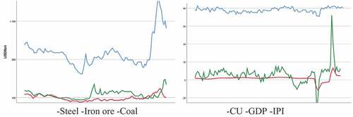
Steel, iron ore and coking coal price series are obtained from industrial resources. Consumer price index (CPI) and producer price index (PPI) of Türkiye are selected as inflation indicators. For capacity utilization (CU) and industrial production index (IPI); steel, automotive, main steel and similar industrial aggregated indexes are taken into account. Europe, OECD and USA GDP and GDP per capita series are taken into consideration. Backward elimination approach is employed to reduce the number of candidate explanatory variables (Makridakis & Wheelwright SC, 1997). See Table 1 and 2.

Table 1. Unit root test

Unit root test	Level	Steel (predicted variable)			Iron ore (explanatory v)
		t	p	Break	t	p	Break
Augmented Dickey–Fuller	0	−2.06	0.3		−2.4	0.2
Augmented Dickey–Fuller	1	−5.37	0		−8.4	0
Philips–Perron	0	−1.6	0.5		−1.9	0.3
Philips–Perron	1	−6.75	0		−8.3	0
Breakpoint	0	−7.82	.01	2020/10	−3.1	0.6	2020/04
Breakpoint	1				−9.9	<.01	2021/07

Table 2. Data Set

Variable	Explanation	Source
Steel price	Cold Rolled flat steel	Industrial
Iron ore price	IODEX 62 Fe CFR China	Industrial
Coking coal price	HCC 64 Mid Vol FOB Australia	Industrial
Inflation	Consumer Price Index (CPI)	TCMB
Capacity Utilization (CU)	CU of main metal industry	TUIK
GDP	GDP of OECD	FRED
Industrial Production	Industrial Production Index (IPI)	TUIK

FRED: Federal Reserve Economic Data

TCMB: Central Bank of the Republic of Türkiye

TUIK: Turkish Statistical Institute

The analysis employs monthly data from February 2012 to November 2020. The justification/explanation of the choice of the study period: The original choice of study period was February 2012 to November 2021, to have the most recent, up-to-date data with which to analyze. However, the periods of the pandemic are removed after structural breaks are determined with unit root testing.

3.1.1. Unit root and breakpoint unit root tests

The unit root test results of both Dickey–Fuller and Philips–Perron suggest that a trend pattern exists in the steel price and iron ore price series; and that first order differencing should be done to remove this trend. There is a breakpoint in the steel price series at period 107, which is at the beginning of the Covid-19 pandemic. Accordingly, the first 105 monthly data points are used in the present analysis; and pandemic period monthly data, which contains the breakpoint, are removed. See Table 1.

3.2. The ARIMA model

An autoregressive moving average (ARMA [p,q]) process includes both an autoregressive function (AR) and a finite moving average (MA) process, where p is the order of autoregressive, q is the order of moving average. Y. Chen et al. (2010) point out that ARMA modelling provides high precision for short-term forecasting, and can be used to reveal the characteristics and dynamic behavior of a time-series. The underlying characteristics of the time-series determine the appropriate model, and can be revealed with an evaluation of the autocorrelation and partial autocorrelation functions; which is a process proposed by Box and Jenkins (1970) to identify the order (d) of an autoregressive integrated moving average [ARIMA (p,d,q)] process, in the case of a non-stationary time-series. In terms of ARIMA model derivation, an autoregressive moving average (ARMA [p,q]) model (equation 3(3) $\mathrm{o}\mathrm{r}\varphi \left(B\right){\tilde{Y}}_t=\theta \left(B\right){\epsilon }_t$(3) ) is constructed from an autoregressive function (AR) and a finite moving average process (MA). The autoregressive process employs lagged predicted variables as explanatory variables (equation 1(1) ${\tilde{Y}}_t={\varphi }_1{\tilde{Y}}_{t-1}+{\varphi }_2{\tilde{Y}}_{t-2}+\dots +{\varphi }_p{\tilde{Y}}_{t-p}+{\epsilon }_t$(1) ); and in a finite moving average process, current and lagged residual series serve as explanatory variables of the model (equation 2(2) ${\tilde{Y}}_t={\epsilon }_t-{\theta }_1{\epsilon }_{t-1}-{\theta }_2{\epsilon }_{t-2}-\dots -{\theta }_q{\epsilon }_{t-q}$(2) ). When differencing is employed an autoregressive integrated moving average [ARIMA (p,d,q)] process is achieved (equation 4(4) ${\omega }_t={\varphi }_1{\omega }_{t-1}+{\varphi }_2{\omega }_{t-2}+\dots {\varphi }_p{\omega }_{t-p}+{\epsilon }_t-{\theta }_1{\epsilon }_{t-1}-{\theta }_2{\epsilon }_{t-2}-\dots -{\theta }_q{\epsilon }_{t-q}$(4) ) in which p indicates the number of lagged periods of predicted variables; and q indicates the amount of residuals included to the model, respectively; and d shows the differencing level of predicted variable (Box & Jenkins, 1970; Box et al., 2016).

(1) ${\tilde{Y}}_t={\varphi }_1{\tilde{Y}}_{t-1}+{\varphi }_2{\tilde{Y}}_{t-2}+\dots +{\varphi }_p{\tilde{Y}}_{t-p}+{\epsilon }_t$(1)

(2) ${\tilde{Y}}_t={\epsilon }_t-{\theta }_1{\epsilon }_{t-1}-{\theta }_2{\epsilon }_{t-2}-\dots -{\theta }_q{\epsilon }_{t-q}$(2)

${\tilde{Y}}_t={\varphi }_1{\tilde{Y}}_{t-1}+{\varphi }_2{\tilde{Y}}_{t-2}+\dots +{\varphi }_p{\tilde{Y}}_{t-p}+{\epsilon }_t-{\theta }_1{\epsilon }_{t-1}-{\theta }_2{\epsilon }_{t-2}-\dots -{\theta }_q{\epsilon }_{t-q}$

(3) $\mathrm{o}\mathrm{r}\varphi \left(B\right){\tilde{Y}}_t=\theta \left(B\right){\epsilon }_t$(3)

If the input of the given process is the differenced series, ARIMA (p,d,q) equation is achieved:

(4) ${\omega }_t={\varphi }_1{\omega }_{t-1}+{\varphi }_2{\omega }_{t-2}+\dots {\varphi }_p{\omega }_{t-p}+{\epsilon }_t-{\theta }_1{\epsilon }_{t-1}-{\theta }_2{\epsilon }_{t-2}-\dots -{\theta }_q{\epsilon }_{t-q}$(4)

where $Y_t$ is the actual value of predicted variable at period t, ${\epsilon }_t$ is the residual, $\mu$ is the level.

$B^m{Y}_t=Y_{t-m}$ represents the lagged terms of predicted series,

$\mathrm{\nabla }{Y}_t=Y_t-Y_{t-1}=\left(1-B\right)Y_t$ is the differenced values,

${\tilde{Y}}_t=Y_t-\mu$ is the differences level,

$\varphi \left(B\right)=1-{\varphi }_{1}B-{\varphi }_2{B}^2-\dots -{\varphi }_p{B}^p$ is the autoregressive component,

${\varphi }_1,{\varphi }_2,\dots ,{\varphi }_p$, and ${\theta }_1,{\theta }_2,\dots ,{\theta }_q$ are coefficients of ARIMA model for autoregressive and residualterms, respectively (Hanke & Wichern, 2014; Kim et al., 2022).

The ARIMA model parameters (p,d,q) are estimated with an error minimizing process. As D. Chen (2011) notes, ARIMA (p,d,q) model building is an empirically driven methodology of systematically identifying, estimating, diagnosing, and forecasting time-series. In other words, the Box–Jenkins ARIMA model estimation approach constitutes a trial-and-error process until obtaining a suitable model and sufficient error reduction.

3.3. The artificial neural network (ANN) model

ANN models have powerful pattern recognition and classification capabilities which make them a powerful tool for forecasting. Multilayer perceptron (MLP) is the main structure used for business forecasting, which has the capability of input-output mapping. MLP may contain several layers of nodes, but three layers is the most common for forecasting. The first layer represent explanatory variables, the second layer is the hidden one and the third layer consists of predicted variable (s; G. Torres-Pruñonosa et al., 2022; Zhang et al., 1998). ANN offers both univariate time-series and multivariate models for forecasting purposes. Armstrong suggests in his forecasting method selection tree that when reliable data exists, multivariate econometric forecasting models should be employed (Armstrong, 2001; Şener, 2015).

In the present study, a feedforward multilayer perceptron network structure is selected for ANN model. The predicted variable and the explanatory variables are standardized or normalized before processing. The predicted variable is employed in third level node and the explanatory variables are entered into the network at first level nodes. The second layer of the network is the hidden one in which the activation function is used. Previous literature mentions that both hyperbolic tangent function and sigmoid function can be used as an activation function in the hidden layer node (M. Zhang, 2008). Weights of the nodes are determined in order to minimize SSE, or MSE in general. Pre-processing of variables and activation function is selected in order to minimize SSE, in the present study.

3.4. Generalized reduced gradient (GRG) algorithms

Generalized reduced gradient (GRG) algorithms (L. L. Lasdon et al., 1974) are utilized to solve nonlinear mathematical models with an objective function to be maximized or minimized, subject to given constraints. It is a gradient based algorithm in which the objective function and constraints can have a nonlinear nature. An objective function value is optimized by searching the steepest descent to the best solution by using a quasi-Newton method for the determination of the minimum gradient. When finding an optimum solution is not allowed by the sophistication of a particular optimization model, a good solution in the feasible region, close to an optimum one, can be determined by GRG algorithm. GRG is mainly used for modelling and solving multivariable models along with successive linear programming, under the operations research discipline. With regard to exponential smoothing methods, GRG algorithm optimizes alpha, beta and gamma weights for level, trend and seasonality estimation functions, respectfully (L. S. L. S. Lasdon et al., 1978). The GRG algorithm technique has been applied in different arenas, such as water resource engineering, load forecasting and fall velocity, for optimizing forecast error parameters mean absolute percentage error (MAPE), sum of squared estimate of errors (SSE) and root mean squared error (RMSE; Shivashankar et al., 2022).

The general form nonlinear model which can be solved by GRG is presented below:

$Minimize\left(ormaximise\right)f\left(X\right)$ $subjectto$ $g_i\left(X\right)=0i=1,2,\dots ,m$ $l_i\le X_i\le u_{i}i=1,2,\dots ,n\mathrm{w}\mathrm{h}\mathrm{e}\mathrm{r}\mathrm{e}{\mathrm{X}}_{\mathrm{i}}\mathrm{a}\mathrm{n}ndimensional\mathrm{v}\mathrm{e}\mathrm{c}\mathrm{t}\mathrm{o}\mathrm{r}.$

GRG algorithm can be used for minimizing model fit statistics, such as MAPE and RMSE, in the determination of the component model forecast weights of the combination forecast, as in the present analysis. Using exclusively in sample data (which is prior to the out of sample forecast period), the present study minimizes MAPE with the GRG algorithm to determine the weights of the out of sample component model forecasts to form an out of sample combination forecast (with the constraint of the weights summing to one, and nonnegative, in the restricted model case:

$MinimizeMAPE\left(X_i\right)where{X}_{i}areweightsofforecasts$

$\left(subjectto\sum X_i=1;and{X}_{i}arenonnegative,intheconstrainedmodelcase\right).$

3.5. Combining methods

3.5.1. Tests of independent information

In the present study, a combining model is formulated in two alternate ways, as indicated above: (1) Using weighted least squares (WLS) estimated regression coefficients (in sample) as forecast weights for the combining model (out of sample). The regressions are alternately run unrestricted and restricted (in which the constant is suppressed and the estimated coefficients are restricted to be nonnegative and to sum to one; (2) Employing a generalized reduced gradient algorithm (GRG) technique (in sample) to estimate the component model forecast weights for the out of sample combination forecasts; with the GRG model alternately run unrestricted and restricted (such that weights are restricted to be nonnegative and to sum to one.)

To begin, following Bates and Granger (1969), C. Granger and Newbold (1975), and Fair and Shiller (1990), the procedure we are proposing in this paper is to run an in-sample regression for the two forecast sources and test the hypothesis that the model 1 (ARIMA-TF) estimated-coefficient = 0; and the hypothesis that model 2 (ANN) estimated-coefficient = 0. The former hypothesis is that model l’s (ARIMA-TF) forecasts contain no information, relevant to forecasting, not in the constant term and in model 2 (ANN). The latter hypothesis is that model 2ʹs forecasts (ANN) contain no information not in the constant term and in model 1 (ARIMA-TF). Paraphrasing Fair and Shiller, and for the case of two component forecasting models (as in the present analysis), if the estimated in-sample regression coefficients are both zero then neither model contains any information useful for out-of-sample forecasting. If both estimated coefficients are nonzero, then it would appear that both models contain independent information useful for out-of-sample forecasting. If both models contain information, but the information in, say, model 1 is completely contained in model 2, and model 2 contains further relevant information as well, then the model 2 estimated coefficient should be nonzero but not the model 1 estimated coefficient. If both models contain the same information, then the forecasts are perfectly correlated and both estimated coefficients are not separately identified.

In the present study, a weighted least squares (WLS) regression of actual (realized) steel prices (in sample values [80%]) against the in sample steel price forecasts generated separately by the ARIMA-TF and the ANN models (employing in sample data), is implemented in the following fashion:

(5) $Y_t={\mathit{B}}_0+\hspace{0.17em}{\mathit{B}}_1\left({\hat{Y}}_{t\left[\mathit{A}\mathit{R}\mathit{I}\mathit{M}\mathit{A}-\mathit{T}\mathit{F}\right]}\right)+\hspace{0.17em}{\mathit{B}}_2\left({\hat{Y}}_{t\left[\mathit{A}\mathit{N}\mathit{N}\right]}\right)\hspace{0.17em}+\hspace{0.17em}{\epsilon }_t$(5)

Where,

$Y_t$ = the actual (realized) steel price for period t from the in sample data set;

${\hat{Y}}_{t\left[\mathit{A}\mathit{R}\mathit{I}\mathit{M}\mathit{A}-\mathit{T}\mathit{F}\right]}$ = the in sample forecasts generated by the ARIMA-TF model using in sample data;

${\hat{Y}}_{t\left[\mathit{A}\mathit{N}\mathit{N}\right]}$ = the in sample forecasts generated by the ANN model using in sample data;

parameters ${\mathit{B}}_0,\hspace{0.17em}{\mathit{B}}_1\mathit{a}\mathit{n}\mathit{d}{\mathit{B}}_2$ are fixed; ${\epsilon }_t$= error term; E [${\epsilon }_t$] = 0.

As noted above, the in-sample regression is alternately run with unrestricted WLS and restricted WLS (in which the constant is suppressed and the estimated regression coefficients are constrained to be nonnegative, and to sum to one).

If the estimated regression coefficients ${\mathit{B}}_1\mathit{a}\mathit{n}\mathit{d}{\mathit{B}}_2$ are nonzero and separately identified, then this would indicate that both models contain independent information content and are thus useful in forming a combining model (Bates & Granger, 1969; C. C. Granger & Newbold, 1975; Fair & Shiller, 1990). As our empirical analysis indicates, this is the case in the present analysis. (See, Table 3 and 5 below.) Subsequently, the in sample estimated regression coefficients $({\mathit{B}}_1\mathit{a}\mathit{n}\mathit{d}{\mathit{B}}_2$) are used as weights for the out of sample component model (ARIMA-TF and ANN) forecasts to generate out of sample combination forecasts of steel prices.

Table 3. ARIMA-TF (1, 1, 0) forecast of in sample (out of sample) data

ARIMA(1,1,0) Model			Coefficient	SE	t-stat	Sig.
Steel price	AR	Lag 1	0.247	0.105	2.348	0.021
Iron ore	Numerator	Lag 0	1341	0.308	4.360	0.000

Table 4. ANN forecast of in sample (out of sample) data

Explanatory Variable	Weight
Iron ore	0.511
Coal	0.018
Inflation	0.048
CU	0.260
GDP	0.153
IPI	0.010

Table 5. WLS regressions of in sample data: $Y_t={\mathit{B}}_0+\hspace{0.17em}{\mathit{B}}_1\left({\hat{Y}}_{t\left[\mathit{A}\mathit{R}\mathit{I}\mathit{M}\mathit{A}-\mathit{T}\mathit{F}\right]}\right)+\hspace{0.17em}{\mathit{B}}_2\left({\hat{Y}}_{t\left[\mathit{A}\mathit{N}\mathit{N}\right]}\right)\hspace{0.17em}+\hspace{0.17em}{\epsilon }_t$

Model		Coefficient	Std. Error	t-stat	Sig.
Unconstrained	(Constant)	−4839	12,669	− .382	0.703
	ARIMA-TF forecasts	0.365	0.054	6.785	0.000
	ANN forecasts	0.642	0.056	11.543	0.000
Constrained	ARIMA-TF forecasts	0.375	N/A	N/A	N/A
	ANN forecasts	0.625	N/A	N/A	N/A

3.5.2. Combination forecasts

Following Bischoff (1989), a combination forecast (${\hat{Y}}_c$) may be expressed as a linear combination of individual model forecasts as follows:

(6) ${\hat{Y}}_c={\mathit{w}}_0+{\sum }_{i=1}^k{\mathit{w}}_i\left({\hat{Y}}_{it}\right)$(6)

where there are k component forecasting models;

And where ${\mathit{w}}_0$ is set to zero and the weights are constrained to be nonnegative and sum to one in the restricted model case.

In the present study, the WLS combining model is constructed by forming a weighted average of both ARIMA-TF and ANN model forecasts (out of sample) as follows:

(7) ${\hat{Y}}_{ct\left[WLS\right]}={\mathit{w}}_0+\hspace{0.17em}{\mathit{w}}_1\left({\hat{Y}}_{t\left[\mathit{A}\mathit{R}\mathit{I}\mathit{M}\mathit{A}-\mathit{T}\mathit{F}\right]}\right)+\hspace{0.17em}{\mathit{w}}_2\left({\hat{Y}}_{t\left[\mathit{A}\mathit{N}\mathit{N}\right]}\right)$(7)

${\hat{Y}}_{ct\left[WLS\right]}$ stands for the out of sample combination forecast formed with estimated regression coefficients from the weighted least squares [WLS] regression (in sample); ARIMA-TF refers to the out of sample forecast made by the transfer function ARIMA model; ANN refers to the out of sample forecast from artificial neural network (ANN) model; w₁,w₂ are the proportional weights, which are the estimated regression coefficients ${\mathit{B}}_1\mathit{a}\mathit{n}\mathit{d}{\mathit{B}}_2$ from the in sample WLS regressions of Eq. 1(1) ${\tilde{Y}}_t={\varphi }_1{\tilde{Y}}_{t-1}+{\varphi }_2{\tilde{Y}}_{t-2}+\dots +{\varphi }_p{\tilde{Y}}_{t-p}+{\epsilon }_t$(1) . Note that WLS combinations are formed alternately using unrestricted and restricted estimated regression coefficients (in sample) as component forecast weights for the out of sample combination forecast, as indicated above.

The GRG combining model is constructed by forming a weighted average of both ARIMA-TF and ANN model forecasts (out of sample) using a generalized reduced gradient algorithm (GRG) technique (in sample) to estimate the component model forecast weights (with the forecast weights also constrained to be nonnegative and to sum to one, in the restricted case):

(8) ${\hat{Y}}_{ct\left[GRG\right]}={\mathit{w}}_1\left({\hat{Y}}_{t\left[\mathit{A}\mathit{R}\mathit{I}\mathit{M}\mathit{A}-\mathit{T}\mathit{F}\right]}\right)+\hspace{0.17em}{\mathit{w}}_2\left({\hat{Y}}_{t\left[\mathit{A}\mathit{N}\mathit{N}\right]}\right)$(8)

Where,

${\hat{Y}}_{ct\left[GRG\right]}$ stands for the out of sample combination forecast made with component model forecast weights generated by the generalized reduced gradient algorithm (GRG) technique (in sample); ARIMA-TF refers to the out of sample forecast made by the transfer function ARIMA model; ANN refers to the out of sample forecast generated by the artificial neural network (ANN) model; w₁,w₂ are the proportional weights which are estimated by the generalized reduced gradient algorithm (GRG) technique (in sample). Note that the GRG combinations are formed alternately using unrestricted and restricted weights for the out of sample combination forecast, as indicated above.

To summarize, the present study calculates the combination-forecast weights using WLS and applies in turn each of two variations regarding the regression restrictions: (1) WLS with a constant term and the coefficients unrestricted; (2) WLS with the constant term suppressed and the coefficients constrained to be nonnegative and sum to one.

Each set of estimated coefficients is then alternately employed as forecast weights to form simulated, ex-ante out-of-sample combination forecasts of steel price.

The present study also calculates the combination-forecast weights using the GRG method and applies in turn each of two variations regarding the forecast weights: (1) unrestricted; (2) constrained to be nonnegative and sum to one.

Each set of estimated weights is then alternately employed to form simulated, ex-ante out-of-sample combination forecasts of steel price.

These two different combining models’ (WLS and GRG) forecasts are generated and compared to each other (and to the component model forecasts) to determine if there is a superior method.

3.5.3. Significance tests of differences in forecast error

While forecast accuracy measures such as root mean square error (RMSE) or mean absolute percentage error (MAPE) can be used to rank or order forecasting models in terms forecast accuracy, the statistical significance of the differences in forecast error between forecast models should also be taken into account. The present analysis utilizes three such tests: The Diebold–Mariano (DM) test, the Harvey–Leybourne–Newbold (HLN) test and the Wilcoxon signed rank test are each employed for testing the null hypothesis that there is no statistically significant difference between an error series of two forecasts. The DM test, initially published in 1995, names the squared differences of error terms as a loss differential and requires it to be covariance stationary (Diebold, 2015; Diebold & Mariano, 1995). The HLN statistic is an adaptation of the DM test (Harvey et al., 1997). Both the DM and HLN statistics provide similar information regarding differences in forecast error between two forecasting models. The nonparametric Wilcoxon signed rank test also compares the absolute error terms of two forecast models (Wilcoxon, 1945) by calculating the differences in each row and ranking them according to magnitude.

3.5.4. Objectives and Statement of Hypotheses

The first objective is to determine whether the employment of the ARIMA-TF model of the present study leads to enhanced forecast accuracy over the employed ANN model. Thus, the first null hypothesis (H₀) to be tested, H₀₁: There is no statistically significant difference between ARIMA-TF and ANN, in forecasting steel price.

The second objective is to determine whether the employment of the ARIMA-TF model of the present study leads to enhanced forecast-accuracy over the GRG combining model (unrestricted). Thus, the second null hypothesis to be tested, H₀₂: There is no statistically significant difference between ARIMA-TF and GRG (unrestricted), in forecasting steel price.

The third objective is to determine whether the employment of the ARIMA-TF model of the present study leads to enhanced forecast-accuracy over the WLS combining model (unrestricted). Thus, the third null hypothesis to be tested, H₀₃: There is no statistically significant difference between ARIMA-TF and WLS (unrestricted), in forecasting steel price.

The fourth objective is to determine whether the employment of the ARIMA-TF model of the present study leads to enhanced forecast-accuracy over the GRG combining model (constrained). Thus, the fourth null hypothesis to be tested, H₀₄: There is no statistically significant difference between ARIMA-TF and GRG (constrained), in forecasting steel price.

The fifth objective is to determine whether the employment of the ARIMA-TF model of the present study leads to enhanced forecast-accuracy over the WLS combining model (constrained). Thus, the fifth null hypothesis to be tested, H₀₅: There is no statistically significant difference between ARIMA-TF and WLS (constrained), in forecasting steel price.

The sixth objective is to determine whether the ANN model of the present study leads to enhanced forecast-accuracy over the GRG combining model (unrestricted). Thus, the sixth null hypothesis to be tested, H₀₆: There is no statistically significant difference between ANN and GRG (unrestricted), in forecasting steel price.

The seventh objective is to determine whether the ANN model of the present study leads to enhanced forecast-accuracy over the WLS combining model (unrestricted). Thus, the seventh null hypothesis to be tested, H₀₇: There is no statistically significant difference between ANN and WLS (unrestricted), in forecasting steel price.

The eighth objective is to determine whether the ANN model of the present study leads to enhanced forecast-accuracy over the GRG combining model (constrained). Thus, the eighth null hypothesis to be tested, H₀₈: There is no statistically significant difference between ANN and GRG constrained, in forecasting steel price.

The ninth objective is to determine whether the ANN model of the present study leads to enhanced forecast-accuracy over the WLS combining model (constrained). Thus, the ninth null hypothesis to be tested, H₀₉: There is no statistically significant difference between ANN and WLS constrained, in forecasting steel price.

The tenth objective is to determine whether the unrestricted GRG combining model outperforms the unrestricted WLS combining model of the present study. Thus, the tenth null hypothesis to be tested, H₀₁₀: There is no statistically significant difference between GRG (unrestricted) and WLS (unrestricted), in forecasting steel price.

The eleventh objective is to determine whether the unrestricted GRG combining model outperforms the constrained GRG combining model of the present study. Thus, the eleventh null hypothesis to be tested, H₀₁₁: There is no statistically significant difference between GRG (unrestricted) and GRG constrained, in forecasting steel price.

The twelfth objective is to determine whether the unrestricted GRG combining model outperforms the constrained WLS combining model of the present study. Thus, the twelfth null hypothesis to be tested, H₀₁₂: There is no statistically significant difference between GRG (unrestricted) and WLS constrained, in forecasting steel price.

The thirteenth objective of the present analysis is to determine whether the unrestricted WLS combining model outperforms the constrained GRG combining model of the present study. Thus, the thirteenth null hypothesis to be tested, H₀₁₃: There is no statistically significant difference between WLS (unrestricted) and GRG constrained, in forecasting steel price.

The fourteenth objective of the present analysis is to determine whether the unrestricted WLS combining model outperforms the constrained WLS combining model of the present study. Thus, the fourteenth null hypothesis to be tested, H₀₁₄: There is no statistically significant difference between WLS (unrestricted) and WLS constrained, in forecasting steel price.

Lastly, the fifteenth objective of the present analysis is to determine whether the constrained GRG combining model outperforms the constrained WLS combining model of the present study. Thus, the fifteenth null hypothesis to be tested, H₀₁₅: There is no statistically significant difference between GRG constrained and WLS constrained, in forecasting steel price.

4. Empirical results and discussion

4.1. Empirical results

To begin, for the analysis of the full data set, which includes monthly data from February, 2012 to November, 2020, divided into 88 in sample periods and 17 out of sample periods: For each component forecasting model (ARIMA-TF and ANN) the present study generates both in sample steel-price forecasts and out of sample steel-price forecasts. (See, Tables 3 and 4 below; no separate tables are presented for the out of sample forecasts, as they are the same.)

With regard to the analysis of the full data set: Regarding the in sample WLS regressions of realized values (monthly price) against predicted values of the two component models (ARIMA-TF and ANN): The estimated regression coefficients are positive and significant with regard to the unrestricted model case. In the restricted model case, the estimated regression coefficients are constrained to be nonnegative and sum to one.¹ The values for these estimated regression coefficients are presented in Table 5 below.

The in sample estimated regression coefficients from both the unrestricted and restricted regressions are then alternately employed as weights to form a weighted average of the out of sample component model steel-price forecasts (ARIMA-TF and ANN).

With regard to the full data set (monthly data from February, 2012 to November, 2020), a combining model is also formed using in sample generated weights that are estimated by the generalized reduced gradient (GRG) algorithm method. This optimization (in-sample forecast-error minimizing [MAPE]) component-forecast weight-determination method is also implemented unrestricted and restricted (with the weights constrained to be nonnegative and sum-to-one in the restricted case.) The estimated values for these weights are presented in Table 7 below.

The in sample estimated weights generated from both the unrestricted and restricted GRG algorithm method are then alternately employed to form a weighted average of the out of sample component model steel-price forecasts (ARIMA-TF and ANN).

(Note: The present analysis does the same above analysis for the two sub segments of the data set. See below.)

For each set of in sample and out of sample forecasts generated by a given model, the current study calculates the mean absolute percentage error (MAPE) and the root mean square error (RMSE) (See, Tables 6 and 7 below).

Table 6. Residual measures of in sample forecasts

Type	Model	MAPE	RMSE	Explanatory Variables
Component Forecasts	ARIMA TF	2.88%	26.20	(1,1,0) Iron ore Lag0
	ANN	2.57%	19.82	Iron ore, Coal, CU, CPI, IPI, GDP

Table 7. Residual measures of out of sample forecasts

Type	Model	MAPE %	RMSE	Weights
				ARIMA	ANN
Component Forecasts	ARIMA TF	6.68	42.68
	ANN	10.67	68.19
Combination Forecasts	GRG unconstrained	6.32	45.38	0.383	0.616
	GRG constrained	6.13	43.66	0.429	0.571
	WLS unconstrained	6.39	46.01	0.370	0.629
	WLS constrained	6.52	46.97	0.357	0.643

The predicted variable steel price and explanatory variable iron ore price are first order differenced according to unit root test results. Six explanatory variables are fit into the ARIMA model, but iron ore price is the only significant one. The ARIMA-TF (1,1,0) with explanatory variable iron ore price produced the best error measures among all other univariate, multivariate and seasonal ARIMA models (see, Table 3). (Note: Once explanatory variables are fit into the ARIMA model it becomes an ARIMA-TF model.)

As mentioned above in section 3 in more detail, all ANN models are constituted with a three-layer perceptron. The first layer is for explanatory variables, the second layer is the hidden one and the third layer employs the dependent variable (steel price). Considering SSE measures from in sample data, standardized, normalized and adjusted normalized data sets are used. Interval offset is selected as 0.1, 0.15 or 0.20.

Both ARIMA-TF and ANN models reveal that iron ore price is the most significant determinant of steel price in the given period (See, Tables 3 and 4, respectively).

In the Table 5, the former model is estimated without constraints; in the latter model however, the constant is suppressed and the coefficients are constrained to be nonnegative and sum to one.

Table 6 indicates that the ANN model outperforms the ARIMA-TF model, by both the MAPE and RMSE measures, with regard to the in sample period.

In contrast to the results presented in Table 6, Table 7 indicates that the ARIMA-TF model outperforms the ANN model, with regard to the out of sample period. However, the out of sample combination forecasts formed with both the WLS and GRG approaches produced remarkably better forecasting performance than the ANN model, and slightly better than ARIMA-TF model, according to the MAPE results.

Table 7 also indicates that the ANN model has the greater weight in all out of sample combination models. There are two possible explanations for the greater weight of the ANN model: One, is that the ANN model produced lower forecast errors (with regard to both MAPE and RMSE measures) for the in sample period, during which the forecast weights are generated; and this information was somehow processed by the study’s weight generating mechanisms (WLS and GRG). Two, the second explanation is that the ANN model contains six explanatory variables, compared to one for the ARIMA-TF model; and thus may have contributed a greater depth of independent information to the combining model.

Marked comparison values in Table 8 represent the existence of significant differences between given forecasts, according to the nonparametric Wilcoxon signed rank test.

Table 8. Wilcoxon signed-rank test for out of sample forecasts

	ARIMA	ANN	GRG	WLS	GRG constrained
ANN	−2.059^b
	0.039
GRG	−0.071^b	−3.574^c
	0.943	0.000
WLS	−0.071^b	−3.574^c	−1.633^b
	0.943	0.000	0.102
GRG constrained	−0.071^c	−3.479^c	−1.349^b	−1.444^b
	0.943	0.001	0.177	0.149
WLS constrained	−0.213^b	−3.574^c	−2.438^b	−3.101^c	−1.728^b
	0.831	0.000	0.015	0.002	0.084

The test results which report significant differences in the compared forecasts are marked in Table 9. The DM and HLN tests presented same results for all comparisons except the WLS constrained and WLS unconstrained combining models. According to the HLN test, there is a difference between them; however, the DM test indicates no significant difference between those given forecasts. Considering the fact that significances of both WLS constrained and unconstrained model are close to the decision threshold, the present study concludes that DM and HLN produced consistent results for the given data set.

Table 9. Diebold–Mariano (DM) and Harvey–Leybourne–Newbold (HLN) results for out of sample forecasts

	ARIMA		ANN		GRG		WLS		GRG cons		WLS cons
ARIMA			HLN	−1.58	HLN	−0.17	HLN	−0.21	HLN	−0.06	HLN	−0.26
			p	0.13	p	0.87	p	0.84	p	0.95	p	0.80
ANN	DM	−1.39			HLN	4.95	HLN	5.01	HLN	4.78	HLN	5.16
	p	0.17			p	0.00	p	0.00	p	0.00	p	0.00
GRG	DM	−0.15	DM	4.35			HLN	−2.94	HLN	2.87	HLN	−2.45
	p	0.88	p	0.00			p	0.01	p	0.01	p	0.03
WLS	DM	−0.18	DM	4.40	DM	−2.58			HLN	2.89	HLN	−2.19
	p	0.85	p	0.00	p	0.01			p	0.01	p	0.043
GRG cons	DM	−0.06	DM	4.20	DM	2.52	DM	2.54			HLN	−2.67
	p	0.96	p	0.00	p	0.01	p	0.01			p	0.02
WLS cons	DM	−0.23	DM	4.54	DM	−2.15	DM	−1.93	DM	−2.35
	p	0.82	p	0.00	p	0.03	p	0.054	p	0.02

The Wilcoxon, DM and HLN tests all indicate that ANN model forecasts are significantly different from other models’ forecasts; and that the ARIMA-TF model produced similar results as other models.

The below results reported in Table 10 indicate that, in general, the accuracy of the ARIMA-TF model forecasts is not significantly different than that of the combining model forecasts of the present study; with the combining models performing slightly better than the ARIMA-TF model (see the MAPE results reported in Table 7 above). However, the results reported in Table 10 indicate that the accuracy of the ANN model forecasts is significantly different than that of the combining model forecasts; with the combining models performing much better than the ANN model (see the MAPE results reported in Table 7 above). Thus, the results reported in Table 10 are consistent with the forecast accuracy measures reported in Table 7, which indicate that the accuracy of the different combination models is slightly better that of the ARIMA-TF model forecasts, but far more precise than that of the ANN model, according to MAPE scores. The above results reported in Table 10 also indicate that the differences in forecast accuracy between the various pairs of combination models can be viewed as slight; which is also consistent with the respective MAPE scores reported in Table 7.

Table 10. Hypotheses of testing summary

H0i	Null Hypothesis	DM	HLN	Wilcoxon
H01	There is no statistically significant difference between ARIMA-TF and ANN	accept	accept	reject
H02	There is no statistically significant difference between ARIMA-TF and GRG (unrestricted)	accept	accept	accept
H03	There is no statistically significant difference between ARIMA-TF and WLS (unrestricted)	accept	accept	accept
H04	There is no statistically significant difference between ARIMA-TF and GRG constrained	accept	accept	accept
H05	There is no statistically significant difference between ARIMA-TF and WLS constrained	accept	accept	accept
H06	There is no statistically significant difference between ANN and GRG (unrestricted)	reject	reject	reject
H07	There is no statistically significant difference between ANN and WLS (unrestricted)	reject	reject	reject
H08	There is no statistically significant difference between ANN and GRG constrained	reject	reject	reject
H09	There is no statistically significant difference between ANN and WLS constrained	reject	reject	reject
H010	There is no statistically significant difference between GRG (unrestricted) and WLS (unrestricted)	reject	reject	accept
H011	There is no statistically significant difference between GRG (unrestricted) and GRG constrained	reject	reject	accept
H012	There is no statistically significant difference between GRG (unrestricted) and WLS constrained	reject	reject	reject
H013	There is no statistically significant difference between WLS (unrestricted) and GRG constrained	reject	reject	accept
H014	There is no statistically significant difference between WLS (unrestricted) and WLS constrained	accept	reject	reject
H015	There is no statistically significant difference between GRG constrained and WLS constrained	reject	reject	reject

A comparison of the DM, HLN, and Wilcoxon tests, suggests that the DM and HLN tests are more sensitive to slight differences in forecast error than the Wilcoxon test. The DM and HLN tests produced results similar to each other.

4.1.1. Sub segment empirical results

As mentioned above, the total data set is divided into two, approximately equal sub segments (the first with 40 in sample and 9 out of sample periods; the second with 43 in sample and 8 out of sample periods). Weighted least squares (WLS) regressions are run over the in-sample data set, for each of the two sub segments of the data set. The results of these regressions are reported in Table 11 below, which indicate that the estimated model coefficients are significantly positive in the unrestricted case; and constrained to be nonnegative and sum to one in the restricted case.²

Table 11. WLS regression results for in sample data of sub segments $Y_t={\mathit{B}}_0+\hspace{0.17em}{\mathit{B}}_1\left({\hat{Y}}_{t\left[\mathit{A}\mathit{R}\mathit{I}\mathit{M}\mathit{A}-\mathit{T}\mathit{F}\right]}\right)+\hspace{0.17em}{\mathit{B}}_2\left({\hat{Y}}_{t\left[\mathit{A}\mathit{N}\mathit{N}\right]}\right)\hspace{0.17em}+\hspace{0.17em}{\epsilon }_t$

Data	Model	Variable	Coefficient	Std. Error	t-stat	Sig.
First half of data	Unconstrained	(Constant)	−34,101	13,771	−2.476	0.018
		ARIMA-TF forecasts	0.265	0.096	2.750	0.009
		ANN forecasts	0.785	0.093	8.464	0.000
	Constrained	ARIMA-TF forecasts	0.072	N/A	N/A	N/A
		ANN forecasts	0.928	N/A	N/A	N/A
Second half of data	Unconstrained	(Constant)	−3.169	55.685	−.057	0.955
		ARIMA-TF forecasts	0.704	0.098	7.170	0.000
		ANN forecasts	0.304	0.133	2.289	0.028
	Constrained	ARIMA-TF forecasts	0.434	N/A	N/A	N/A
		ANN forecasts	0.566	N/A	N/A	N/A

These in sample estimated regression coefficients, for each of the two in sample sub sets, are then employed as weights to form a weighted average of the out-of-sample component model steel-price forecasts (ARIMA-TF and ANN), for each of the two subsets of data. (See, Table 11 below for the sub sample forecasting results.)

The present study also forms a combining model by the generalized reduced gradient algorithm (GRG) method for each of the two sub segments of the data set. The estimated values for these sub-segment in- sample determined weights are presented in Table 11 below.

Considering the in sample results for sub segments data sets presented in Table 12, the first segment’s error measures are lower, and the second segment’s error measures are higher than the respective results of main, full data set. Note that the ARIMA-TF model outperforms the ANN model in the first sub segment; and the ANN model outperforms the ARIMA-TF model in the second sub segment. Iron ore remains the most important explanatory variable in the sub segment data sets.

Table 12. Residual measures of in sample data for sub segments

Data	Model	MAPE	RMSE	Explanatory Variables
First half of the data	ARIMA-TF	2.15%	20.24	(0,1,0) Iron ore
	ANN	1.63%	13.88	Iron ore, Coal, CU, CPI, IPI, GDP
Second half of the data	ARIMA TF	3.70%	30.32	(0,1,0) Iron ore
	ANN	4.54%	36.08	Iron ore, Coal, CU, CPI, IPI, GDP

4.2. Discussion

With regard to the weighted least squares (WLS) in sample regression tests of independent information (equation 1(1) ${\tilde{Y}}_t={\varphi }_1{\tilde{Y}}_{t-1}+{\varphi }_2{\tilde{Y}}_{t-2}+\dots +{\varphi }_p{\tilde{Y}}_{t-p}+{\epsilon }_t$(1) ), by dint of the unrestricted regression model, both the ARIMA-TF and ANN component model in sample forecasts are found to contain independent information, as indicated by the significantly positive estimated regression coefficients, respectively (See, Table 5 for the full data set regression results; and Table 11 for the regression results of the sub segment data sets). Thus, the present study rejects the null hypothesis that the ARIMA-TF model estimated in sample regression coefficient = 0; and the null hypothesis that the ANN model estimated in sample regression coefficient = 0 (as stated in the section 3 Methodology). As noted above (in section 3), if the estimated regression coefficients are nonzero and separately identified, then this would indicate that both models contain independent information content and are thus useful in forming a combining model (Bates & Granger, 1969; Fair & Shiller, 1990; C. Granger & Newbold, 1975). Subsequently, the in sample estimated regression coefficients are used as weights for the out of sample component ARIMA-TF and ANN model forecasts to generate out of sample combination forecasts of steel prices. The present study employed both unrestricted and restricted regression coefficients to form an out of sample combining model (with the coefficients constrained to be nonnegative and to sum to one, and the constant suppressed, in the restricted model) as detailed above in section 3.

The present study also utilized both an unrestricted and restricted GRG algorithm method for determining combination forecast weights. As indicated above, with the restricted GRG method the weights are constrained to be nonnegative and to sum to one.

As reported above, the accuracy of the different combination models (unrestricted and constrained WLS; unrestricted and constrained GRG) is slightly better that of the ARIMA-TF model forecasts, but far more precise than that of the ANN model, according to the forecast accuracy measures (MAPE) scores reported in Table 7.

In the present study, the constrained GRG combining model provided lower error measures than the unconstrained GRG combining model, in general. (See, Tables 6 and 9 for the full data set outcomes; and Table 12 for the outcomes of the sub segment out-of-sample data sets.) The GRG combining model also produced competitive results with the more conventional WLS combining model approach for combination forecasts. (Again, see, Tables 7 and 10 for the full data set outcomes; and Table 13 for the outcomes of the sub segment out-of-sample data sets.) The findings of the present analysis suggest that the GRG combining method is a successful, alternative technique to the WLS combining method, and can also be utilized to improve forecast precision.

Table 13. Residual measures of out of sample data for sub-segments

Data	Model	MAPE %	RMSE	Weights
				ARIMA	ANN
First half of data	ARIMA TF	11.51%	56.61
	ANN	11.79%	55.99
	GRG unconstrained	11.19%	54.00	0.388	0.610
	GRG constrained	11.46%	54.96	0.345	0.655
	WLS unconstrained	17.13%	79.17	0.265	0.785
	WLS constrained	11.72%	55.67	0.072	0.928
Second half of data	ARIMA TF	4.57%	26.68
	ANN	5.08%	30.74
	GRG unconstrained	4.55%	27.22	0.631	0.363
	GRG constrained	4.35%	25.84	0.659	0.341
	WLS unconstrained	4.85%	30.40	0.704	0.304
	WLS constrained	4.54%	26.62	0.434	0.566

Note that for the out of sample period of the second sub segment data set, Table 13 indicates significantly lower forecast error measures for all respective models, compared to those reported for the first sub segment; with the unrestricted GRG model performing best in the first sub segment; and the constrained GRG model performing best in the second sub segment. Note that the weight of the ARIMA-TF forecast is higher than the weight of the ANN forecast in the first three out of four cases in the second sub set; whereas in the first sub segment the ANN model forecast has higher weights in all four cases.

The present study also finds that the WLS combining model approach is more successful when the estimated in sample regression coefficients are constrained to be nonnegative and sum to one, in comparison with the unrestricted WLS combining model approach. See Figure 2. These results are supportive of the previous studies indicated above in section 2 [Clemen (1986), Gunter (1992), Aksu and Gunter (1992), Gunter and Aksu (1997), and Terregrossa (2005), Nowotarski et al. (2014), Terregrossa and Ibadi (2021)], which all found that a constrained regression combining model outperformed the unrestricted regression combining model counterpart.

Figure 2. Vertex line indicating lowest RMSE with forecast weights constrained to be nonnegative and sum to one.

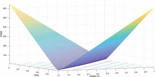
Figure 2 illustrates that constraining the forecast weights in the combining model to be nonnegative and sum to one leads to minimum forecast error, as indicated by the vertex line.

The present study finds that the ANN model produced lower error measures compared to the ARIMA-TF model for in sample periods; whilst the ARIMA-TF model produced better results for out of sample periods.

The present study fills a research gap and breaks new ground with the introduction of the GRG algorithm approach to forming a combining model. The GRG combining method produced slightly more precise forecasting results than WLS method, according to MAPE and RMSE forecast accuracy measures. However, according to Wilcoxon signed rank, DM, and HLN tests, there is no significant difference between the WLS and GRG combining model results. Therefore, the empirical results of the present analysis cannot unequivocally determine which technique is the better combining model approach. Nevertheless, the present study finds that both combining model techniques (GRG and WLS) produced successful (and similar) combination forecast accuracy. Further research is necessary to reveal the comparative performance of both methods.

Last, the present study finds a statistical forecasting technique in the form of an ARIMA-TF model produced competitive results compared with a machine-learning technique in the form of artificial neural network (ANN) method.

5. Conclusions

The present study has developed a model for improved accuracy of steel price forecasts by forming weighted average combinations of forecasts generated separately by a transfer function ARIMA model (ARIMA-TF) and an artificial neural network model (ANN), with the implementation of a constrained generalized reduced gradient algorithm (GRG) technique to estimate the component model forecast weights. These component models (ARIMA-TF and ANN) are chosen for the combination as both models are shown to contribute independent information with regard to steel price determination. The independent information provided by each model partly stems from the fact that the ARIMA model can discern any linear functional relations inherent in the data, but not nonlinear; while the ANN model can discern any nonlinear functional relations inherent in the data. And also, by the fact that the ANN model employs a greater number of explanatory variables.

The present analysis is in part motivated by a research gap in the literature with regard to steel price forecasting: The present study appears to be the first in forming a combining model to enhance accuracy of steel price forecasts. The present analysis is also partly motivated by a methodological gap in the research area of combination forecasting, which the study addresses with the introduction of a constrained generalized reduced gradient algorithm (GRG) technique to estimate the component model forecast weights. The current study finds that the combining model formed with the gradient algorithm approach in which the weights are constrained to be nonnegative and sum to one has the lowest MAPE of all models tested, and overall is found to be very competitive with other models tested in the study. The policy implication for firms that use steel as a major input is to base their hedging decisions on a such a combining model of steel price forecasts as employed in the present study.

One area of future study would be to experiment with different combining methods such as using a hybrid method in which steel price forecasts are first generated with an ARIMA-TF model, and the ARIMA-TF error series is recorded; then an autoregressive neural network (NARNET) model can be employed to model the residuals from the ARIMA model and generate forecasts of the ARIMA-TF error series. The hybrid price forecast is the sum of the ARIMA-TF forecast and the NARNET-generated error forecast. Additionally, a further step may be taken by combining an ARIMA-NARNET (or ARIMA-ANN) hybrid forecast with yet another forecast (for instance, a polynomial regression forecast), employing a constrained gradient algorithm approach (GRG) to determine the component forecast weights. Another idea that may prove useful is to utilize 3-month data periods, as a way to smooth out any noise in monthly data. One limitation of the present analysis stems from the need to eliminate data from the pandemic period, as a result of a structural break as indicated by unit root testing.

Acknowledgments

The authors are grateful for the comments and suggestions provided by the three anonymous reviewers, which led to significant improvements in the manuscript.

Disclosure statement

No potential conflict of interest was reported by the author(s).

Additional information

Funding

The authors received no direct funding for this research.

Notes

1. However, the significance of the restricted regression results can only be inferred from the unrestricted case, as the software utilized in the present study to run constrained WLS regressions [E-views] does not report the t-stat significance test values for the constrained WLS regressions.

2. However, the significance of the results in the restricted case can only be inferred from the unrestricted case, for reasons as explained above with regard to the regression results for the full data set, reported in Table 5 above.

References

- Adli, K. A., & Sener, U. (2021). Forecasting of the U.S. Steel prices with LVAR and VEC models. Business and Economics Research Journal, 12(3), 509–25. https://doi.org/10.20409/berj.2021.335
- Ajupov, A. A., Kurilova A. A, and Ivanov, D. U. (2015). Application of Financial Engineering Instruments in the Russian Automotive Industry. ASS, 11(11). https://doi.org/10.5539/ass.v11n11p162
- Aksu, C., & Gunter, S. I. (1992). An empirical analysis of the accuracy of SA, OLS, ERLS and NRLS combination forecasts. International Journal of Forecasting, 8. https://doi.org/10.1016/0169-2070(92)90005-T
- Armstrong, J. S. (2001). Principles of forecasting A handbook for researchers and practitioners. Springer Science.
- Bates, J. M., & Granger, C. W. J. (1969). The combination of forecasts. Operational Research Society, 20(4), 451–468. https://doi.org/10.1057/jors.1969.103
- Bischoff, C. W. (1989). The combination of macroeconomic forecasts. Journal of Forecasting, Vat, 8(3), 293–314. https://doi.org/10.1002/for.3980080312
- Bodnar, GM et al. (1995). Wharton survey of derivatives usage by US non-financial firms.Financial management,24(2), 104–114.
- Box, G. E. P., & Jenkins, G. M. (1970). Time series analysis: Forecasting and control (1st) ed.). Holden-Day.
- Box, G. E. P., Jenkins, G. M., & Ljung, G. M. (2016). Time series analysis forecasting and control (5th) ed.). Wiley.
- Chen, D. (2011). Chinese automobile demand prediction based on ARIMA model. Proceedings - 2011 4th International Conference on Biomedical Engineering and Informatics, BMEI 2011, 4, 2197–2201. https://doi.org/10.1109/BMEI.2011.6098744
- Chen, Y., Zhao, H., & Yu, L. (2010). Demand forecasting in automotive aftermarket based on ARMA model. 2010 International Conference on Management and Service Science, MASS 2010. https://doi.org/10.1109/ICMSS.2010.5577867
- Chou, M. T. (2013). Review of economics & finance, 3, 90–98.
- Clemen, R. T. (1986). Linear constraints and the efficiency of combined forecasts. Journal of Forecasting, 5(1), 8–31. https://doi.org/10.1002/for.3980050104
- Clemen, R. T. (1989). Combining forecasts: A review and annotated bibliography. International Journal of Forecasting, 5(4), 559–583. https://doi.org/10.1016/0169-2070(89)90012-5
- Cooper, J. P., & Nelson, C. R. (1975). The Ex Ante prediction performance of the St. Louis and FRB-MIT-PENN econometric models and some results on composite predictors. Journal of Money, Credit and Banking, 7(1), 1. https://doi.org/10.2307/1991250
- Diebold, F. X. (2015). Comparing predictive accuracy, twenty years later: A personal perspective on the use and abuse of Diebold–Mariano tests. Journal of Business and Economic Statistics, 33(1), 37–41. https://doi.org/10.1080/07350015.2014.983236
- Diebold, F. X., & Mariano, R. S. (1995). Comparing predictive accuracy. Journal of Business & Economic Statistics, 13(3), 134–144. https://doi.org/10.1016/0169-2070(88)
- Diebold, F. X., & Pauly, P. (1987). Structural change and the combination of forecasts. Journal of Forecasting, 6. https://doi.org/10.1002/for.3980060103
- Drought, S., & McDonald, C. (2011). Forecasting house price inflation: A model combination approach. Reserve Bank of New Zealand Discussion, October, 1–23. http://nzae.org.nz/wp-content/uploads/2011/08/Drought_and_McDonald__Forecasting_House_Price_Inflation.pdf
- Fair, R. C., & Shiller, R. J. (1990). Comparing information in forecasts from econometric models. The American Economic Review, 80(3), 375–389. https://www.jstor.org/stable/2006672
- Granger, C., & Newbold, P. (1975). Economic Forecasting-the atheist's viewpoint. Modelling the economy, 131–147.
- Granger, C. W. J., & Ramanathan, R. (1984). Improved methods of combining forecasts. Journal of Forecasting, 3(2), 197–204. https://doi.org/10.1002/for.3980030207
- Guerard, J. B. (1987). Linear constraints, robust weighing and efficient composite modelling. Journal of Forecasting, 6(3), 193–199. https://doi.org/10.1002/for.3980060305
- Gunter, S. I. (1992). Nonnegativity restricted least squares combinations. International Journal of Forecasting, 8, https://doi.org/10.1016/0169-2070(92)90006-U
- Gunter, S. I., & Aksu, C. (1997). The usefulness of heuristic N(E)RLS algorithms for combining forecasts. Journal of Forecasting, 16(6), 439–462. https://doi.org/10.1002/(sici)1099-131x(199711)16:6<439::AID-FOR624>3.0.CO;2-8
- Hakim, D. (2003). Steel Supplier Is Threatening To Terminate G.M. Shipments. New York Times.
- Hanke, J. E., & Wichern, D. W. (2014). Business forecasting (9th) ed.). Pearson.
- Harvey, D., Leybourne, S., & Newbold, P. (1997). Testing the equality of prediction mean squared errors. International Journal of Forecasting, 13(2), 281–291. https://doi.org/10.1016/S0169-2070(96)00719-4
- Kapl, M., & Müller, W. G. (2010). Prediction of steel prices: A comparison between a conventional regression model and MSSA. Statistics and Its Interface, 3(3), 369–375. https://doi.org/10.4310/sii.2010.v3.n3.a10
- Kim, S., Choi, C.-Y., Shahandashti, M., & Ryu, K. R. (2022). Improving Accuracy in Predicting City-Level Construction Cost Indices by Combining Linear ARIMA and Nonlinear ANNs. Journal of Management in Engineering, 38(2), 2. https://doi.org/10.1061/(asce)me.1943-5479.0001008
- Lasdon, L., Fox, R., & Ratner, M. (1974). Nonlinear optimization using the generalized reduced gradient method. RAIRO - Operations Research - Recherche Opérationnelle, 3(8), 73–103. http://www.numdam.org/item?id=RO_1974__8_3_73_0
- Lasdon, L. S., Waren, A. D., Jain, A., & Ratner, M. (1978). Design and testing of a generalized reduced gradient code for nonlinear programming. ACM Transactions on Mathematical Software (TOMS), 4(1), 34–50. https://doi.org/10.1145/355769.355773
- Liebman, B. H. (2006). Safeguards, China, and the price of steel. Review of World Economics, 142(2), 354–373. https://doi.org/10.1007/s10290-006-0071-y
- Liu X. (2020). Does Industrial Agglomeration Affect the Accuracy of Analysts’ Earnings Forecasts?. AJIBM, 10(05), 900–914. https://doi.org/10.4236/ajibm.2020.105060
- Liu, Z., Wang, Y., Zhu, S., & Zhang, B. (2015). Steel prices index prediction in china based on BP neural network. Springer, 603–608. https://doi.org/10.1007/978-3-662-43871-8
- Lobo, G. (1991). Alternative methods of combining security analysts’ and statistical forecasts of annual corporate earnings. International Journal of Forecasting, 7(1), 57–63. https://doi.org/10.1016/0169-2070(91)
- Makridakis, S. G., Parzen, E., Fildes, R., & Andersen, A. (1984). The forecasting accuracy of major time series methods. John Wiley & Sons.
- Makridakis, S., & Wheelwright SC, H. R. (1997). Forecasting methods and applications. In Forecasting methods and applications (3rd) ed.), (pp. 632). John Wiley & Sons.
- Malanichev, A. G., & Vorobyev, P. V. (2011). Forecast of global steel prices. Studies on Russian Economic Development, 22(3), 304–311. https://doi.org/10.1134/S1075700711030105
- Mancke, R. (1968). The Determinants of Steel Prices in the U.S.: 1947-65. The Journal of Industrial Economics, 16(2), 147. https://doi.org/10.2307/2097798
- Mathews, R. G. (2011). Steel-Price Increases Creep Into Supply Chain. The Wall Street Journal.
- Mir, M., Kabir, H. M. D., Nasirzadeh, F., & Khosravi, A. (2021). Neural network-based interval forecasting of construction material prices. Journal of Building Engineering, 39(February), 102288. https://doi.org/10.1016/j.jobe.2021.102288
- Nelson, C. R. (1972). The prediction performance of the FRB-MIT-PENN model of the U.S. economy. American Economic Association, 62, 5. https://www.jstor.org/stable/1815208
- Nowotarski, J., Raviv, E., Trück, S., & Weron, R. (2014). An empirical comparison of alternative schemes for combining electricity spot price forecasts. Energy Economics, 46, 395–412. https://doi.org/10.1016/j.eneco.2014.07.014
- Rapach, D. E., & Strauss, J. K. (2009). Differences in housing price forecastability across US states. International Journal of Forecasting, 25(2), 351–372. https://doi.org/10.1016/j.ijforecast.2009.01.009
- Şener, U. (2015). Tahmin metodolojisi ve tahmin yöntemi seçimi. Beykoz Akademi Dergisi, 3(1), 85–98. https://dergipark.org.tr/tr/pub/beykozad/issue/52157/682081
- Shivashankar, M., Pandey, M., & Zakwan, M. (2022). Estimation of settling velocity using generalized reduced gradient (GRG) and hybrid generalized reduced gradient–genetic algorithm (hybrid GRG-GA). Acta Geophysica, 0123456789. https://doi.org/10.1007/s11600-021-00706-2
- Stock, J. H., & Watson, M. W. (2004). Combination forecasts of output growth in a seven-country data set. Journal of Forecasting, 23(6), 405–430. https://doi.org/10.1002/for.928
- Terregrossa, S. J. (2005). On the efficacy of constraints on the linear combination forecast model. Applied Economics Letters, 12(1), 19–28. https://doi.org/10.1080/1350485042000307062
- Terregrossa, S. J., & Ibadi, M. H. (2021). Combining housing price forecasts generated separately by hedonic and artificial neural network models. Asian Journal of Economics, Business and Accounting, 21(1), 130–148. https://doi.org/10.9734/ajeba/2021/v21i130345
- Torres-Pruñonosa, J., García-Estévez, P., Raya, J. M., & Prado-Román, C. (2022). How on earth did Spanish banking sell the housing stock? SAGE Open, 12(1), 1. https://doi.org/10.1177/21582440221079916
- Turcic, D., Kouvelis, P., & Bolandifar, E. (2014). Hedging Commodity Procurement in a Bilateral Supply Chain. M&SOM, 17(2), 221–235. https://doi.org/10.1287/msom.2014.0514
- Wilcoxon, F. (1945). Individual comparisons by ranking methods. Biometrics Bulletin, 1(6), 80–83. https://doi.org/10.2307/3001968
- Yuzefovych, I. (2006). Ukrainian industry in transition: Steel price determination model. National University Kyiv-Mohyla Academy.
- Zhang, G.P. Time series forecasting using a hybrid ARIMA and neural network model. Neurocomputing, 50, 159–175.
- Zhang, M. (2008). Artificial higher order neural networks for economics and business. Artificial Higher Order Neural Networks for Economics and Business. https://doi.org/10.4018/978-1-59904-897-0
- Zhang, G., Eddy Patuwo, B., & Y. Hu, M. (1998). Forecasting with artificial neural networks: The state of the art. International Journal of Forecasting, 14(1), 35–62. https://doi.org/10.1016/S0169-2070(97)