Financial stability in the Indonesian monetary policy analysis

Abstract

Financial stability is one of the main factors for a country’s economic sustainability nowadays. Financial instability has adverse effects on the economy which can lead to the financial crisis. This research tries to answer how monetary policy related to Indonesian financial stability in the short and long term, how specific the relations between its parts such as money supply, interest rate, and exchange rate to indonesian financial stability, and which one of these parts that have ways more effective to influence Indonesian financial stability. This research data use time series quarterly as quantitative data in Indonesia. By employing econometric models of error correction on quarter data that consist of the stationary stochastic process, long-run model and cointegration approach and error correction model, this model can indicate how quickly the effect of the money supply, interest rate or exchange rate is fully accepted by the financial stability in the short term. The finding of this study showed that the increase in interest rate began to be able to improve indonesian financial stability responsively in four times the period, namely an increase of one percent in interest rate could increase 0.4161 percent of financial stability in Indonesia.

Keywords:

• financial stability
• money supply
• interest rate
• exchange rate
• error correction model

JEL CLASSIFICATION:

• E44
• E52

PUBLIC INTEREST STATEMENT

Financial stability is one of the main factors for a country’s economic sustainability. Financial instability adversely affects the economy, leading to a financial crisis. This research tries to answer how monetary policy is related to Indonesian financial stability in the short and long-term sense, how specific the relations between its parts, such as money supply, interest rate, and exchange rate to Indonesian financial stability, and which one of these parts that have ways more effective to influences Indonesian financial stability. This study’s finding showed that the interest rate increase began to improve Indonesian financial stability responsively four times. Namely, an increase of one percent in interest rate could increase 0.4161 percent of financial stability in Indonesia.

1. Introduction

Recently, financial stability has become a concern for the central bank and government in an effort to prevent the crisis in the financial sector. In general, financial system can be regarded as stable if it has the capability to intermediate, risk spreading, and make payment; can keep the activities of real sectors and financial system through fund resource allocation and good economic shock absorption; and can support the economic growth and the economy mechanism in pricing (Bank Indonesia, 2018a). Financial instability can be caused by market failure. Market failure can be caused by several factors like monopoly and oligopoly, asymmetrical information, negative externality that causes inhibition of production, increasing marginal cost, and market inefficient such as air pollution, production waste, and so forth. It can be sourced from within the country and abroad. There are risks in financial system activity like credit risk (increase in non-performing loan), liquidity risk (difficulties to provide cash in a certain amount of time), market risk (decrease in investment values), and operational risk (ineffectiveness of internal, human and system processes; Bank Indonesia, 2018a). Wahab et al. (2021) revealed the cointegration relationships of financial stability with structural breaks among consumption-based renewable energy, technological innovation and gross domestic product (Wahab et al., 2022). Likewise, Rahim et al. (2021) and Pattawe et al. (2022) have identified the quantity and quality of natural resources and human resources in economic growth in emerging economies.

The United States financial crisis in 2018, which dubbed a global financial crisis, has domino effects in the global financial market. It was caused by high debt accumulation in mortgage facilitated by securitized banking credit and widely traded in the financial sector. Sub-prime mortgage securities, its structured products, and risky behavior cause stagnancy in high debt (leverage) accumulation that led to the collapsing of all financial systems (Warjiyo & Juhro, 2016). The global financial crisis has an impact on decreasing global market confidence, which can be felt not only by the United States but also in all countries in the active global market. They have to sell their assets at the financial market as a result of the withdrawal of foreign investor funds and declining levels of trust (Bank Indonesia, 2016b). This shock in the financial market can disrupt financial stability.

Monetary policy is expected to have more active roles in Indonesian financial stability. Stabilization efforts can be realized by controlling the money supply, interest rate, and exchange rate. Inflation control is one of the objectives that must be fulfilled in order to implement monetary policy. It has an effect on financial stability. It can be a negative direction to financial stability when its rate has become lower, financial stability has become more stable (Dhal et al., 2011). Nowadays, the government has tried many ways to create financial stability. Financial stability is an important thing because instability bring various bad impacts such as ineffective fund allocation that happened caused by ineffective intermediation so can disrupt economic growth; low level of trust from people regarding financial system that can make investor withdrawing their fund so liquidity risks are getting higher; the cost of economy recovery caused by crisis is getting higher if it tend to crisis with systemic impact and the recovery that not in a short time; ineffective monetary policy caused by its transmission that doesn’t end well (Bank Indonesia, 2018c). It is expected that the policy has positive effects so the financial system can be stable and work well.

Expansive monetary policy leads to an increase in lending, but also a growth in risk-taking behavior and risk aversion which can lead to an increase in bank debt and broker-dealers, and may increase the supply of loans. It causes a decrease in price of risk and contemporary risk. Compression in risk and risk pricing tends to increase expectations of future risk, as it triggers debt due to weak risk management, so that raising concerns about financial instability due to the low-risk premium and low volatility that contribute to the build-up of imbalances namely volatility paradox. Higher debt can increase the vulnerability of the financial system in the form of systemic risk. Empirically, Morris (2010) stated that money supply (m2) significantly affects the dependent variable of aggregate stability index in a negative direction (Morris, 2010). Meanwhile, Albulescu (2012) revealed that economic growth variable and the interest rate have very strong significant effect toward dependent variable namely financial stability which the first has positive direction while the latter has negative one (Albulescu, 2012).

Therefore, this paper tries to analyze the effect of monetary policy toward financial stability in Indonesia during 2006–2015 by using the error correction model approach. Some of the research questions which are developed in this study are how is the short- and long-run relationship of monetary policy toward Indonesian financial stability, and how specific is the relation between the monetary policy parts such as money supply, interest rate, and exchange rate toward Indonesian financial stability and which one of those that has more effective ways to fulfill Indonesian financial stability. By utilizing the two-step Engle-Granger error correction procedure on ten years of quarterly financial stability, money supply, interest rate and exchange rate in Indonesia, this study examines the effect of money supply, interest rate and exchange rate toward financial stability in the short-run and long-run in Indonesia. This model can indicate how quickly the effect of the money supply, interest rate or exchange rate is fully accepted by financial stability in the short term. So, this study can identify monetary policy instruments that most influence the stability of the Indonesian financial system in the long term and short term.

2. Background

The development of the Indonesian interest rate has been declining since 2007. It was caused by stable macroeconomy conditions so the inflation target can be fulfilled and BI can lower its policy rate step by step to push economy activities (Bank Indonesia, 2008). In 2008, the interest rate has been improved until the second quarter and quite stable in the third and fourth quarters. It was caused by the global financial crisis sourced from the United States. Indonesian interest rate is declining in 2009 because there was an encouragement, especially in the improvement of credit supplies, to push real sectors (Bank Indonesia, 2010). The development of inflation and interest rate in Indonesia during 2006Q1-2010Q4 can be seen in Figure 1.

Figure 1. Inflation (%) and Interest Rate (%) in Indonesia, 2006Q1-2010Q4.

Source: Bank Indonesia (processed)

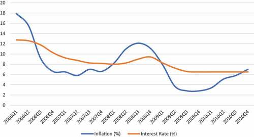
Based on Figure 1, the high inflation rate in Indonesia during 2006 cannot be separated from the increasing prices in fuel and food at the end of 2005. During 2008, its rate was higher than before. It was caused by a high price in global commodities such as fuel and food. The domino effect of the global financial crisis can be felt in the Indonesian inflation rate during this period. The recovery of market confidence in 2009 gives an effect to lower the inflation level and it tends to fluctuate until 2010. Nonetheless, the inflation and interest rate relatively controlled. Indonesia encountered net capital outflow related to the release of domestic financial assets and banking excess liquidity which was relatively high in 2012 (Bank Indonesia, 2013). Indonesia has implemented a range of policies consisting of interest rate policy and some policies (Figure 2).

Figure 2. Inflation (%) and Interest Rate (%) in Indonesia, 2011M1-2018M12.

Source: Bank Indonesia (processed)

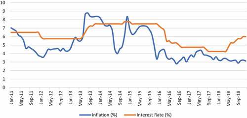
There are three global issues namely lack of clarity over tapering off the fiscal stimulus as signaled by the Fed, uncertainty over global economic recovery, and the prolonged decline in commodity prices in 2013. The domestic economic conditions were affected by the trade and financial channels. Further challenges were posed by the Indonesian economy structure, which lacked the capacity to maintain pace with buoyant domestic demand. As a result, the balance of payments came under mounting pressure, accompanied by rising inflation and weakening in the exchange rate (Bank Indonesia, 2014). In 2015, inflation volatility in Indonesia is influenced by shocks of volatile food and administered prices. One commodity which has big benefaction is chili. Chili has high price instability due to the uneven availability of supply throughout the year (Bank Indonesia, 2016a).

In 2018, Indonesia’s economy faces severe challenges stemming from three global uncertainties. First, slowing global economic growth. Secondly, the increasing Fed Fund Rate is faster and higher than the previous year. Third, the increasing uncertainty in global financial markets due to the US-China trade war. Therefore, the increase in interest rate is directed to provide attractiveness for foreign investment in the domestic financial market. In addition, the policy rate is also pursued to maintain inflation in accordance with its target (Bank Indonesia, 2019). The decline of interest rate was not always followed by inflation increase, on the other hand, it was not always followed by destabilization in financial stability. The development of money supply in Indonesia during 2006Q1-2010Q4 can be seen in Figure 3.

Figure 3. Money Supply (Billions of Rp) in Indonesia, 2006M1-2018M12.

Source: Bank Indonesia (processed)

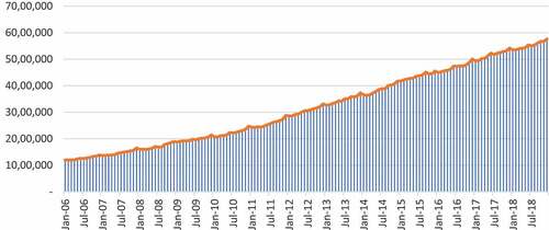
Based on Figure 3, the development of the Indonesian money supply has some positive trends during 2006Q1-2010Q4. It was caused by the increase of the money printing offset by consumption rate, people savings, and inflation rate. In 2007, Bank Indonesia has tried to prove its vital existence by actively facilitating banking financial intermediation in various regions to accelerate the movement of micro, small and medium enterprises, real sectors and its development (Bank Indonesia, 2008). Those efforts led to the money supply in societies has been increased during that year. In 2008, the Indonesian economy has been influenced by global economy turmoil so Bank Indonesia needs to take policies in stabilizing macroeconomy and minimalizing the effects of the global financial crisis on the domestic economy. These policies have been taken care of as an effort to strengthen banking resilience against the global financial crisis and to support real sectors (Bank Indonesia, 2009). That was the reason why the money supply has been increased in 2008. In 2009, increasing money supply has been triggered by the issuance of a 2009 edition of Rp 2,000.00 banknotes to fulfill the need of Rupiah in enough amount, on time, suitable, and circulation worthy in society (Bank Indonesia, 2010).

In 2017, Bank Indonesia seeks to expand circulation of Rupiah issued in the 2016 Emission Year simultaneously with as many as 11 denominations (Bank Indonesia, 2018b). Bank Indonesia is committed to increasing the distribution of money supply to various regions of Indonesia in 2018, including the 3 T regions (the outermost, frontline and disadvantaged regions; Bank Indonesia, 2019). That was the reason why the money supply has been increased from 2017–2018. This increase is not always impacted by the high inflation rate, or on the other hand, it is not always impacted by destabilization in financial stability. The development of the Indonesian exchange rate during 2006Q1-2010Q4 can be seen in Figure 4.

Figure 4. Exchange Rate (IDR/USD) in Indonesia, 2006Q1-2018Q4.

Source: Bank Indonesia (processed)

Based on Figure 4, the development of the Indonesian exchange rate during 2006 was quite stable. It happened because Bank Indonesia tried to balance the supply and demand of foreign exchanges in the money market and its speculation in foreign exchange transactions by co-operating with the government regarding the provision of foreign exchange needs for state-owned enterprises. It also did transaction intervention or sterilization to manage foreign exchange liquidity in the money market, and follow all the activities in the money market and real sector that has an effect on Rupiah currency. The improving performance of Indonesia’s Balance of Payments is also a factor that makes Rupiah currency stable (Bank Indonesia, 2007). The development of the Indonesian exchange rate did not significantly fluctuate in 2007. The integration of the national economy with the economy world causing Bank Indonesia to improve its monitoring quality on transactions in the foreign exchange market and its traffic that can give early warning information regarding perception and behavior-changing of the market participants so it can take preventive measures faster. Interesting yield in domestic financial markets and improving Indonesian risk premium investment has become a factor in the effort to stabilize Rupiah’s currency (Bank Indonesia, 2008).

The development of the Rupiah exchange rate was quite stable in the first until the third quarter and began to depreciate significantly in the fourth quarter of 2008. This depreciation was caused by tight global credit condition and liquidity pressure in financial sector caused by the global liquidity crisis and high demand in domestic credit which most of it were paid by secondary reserves (Bank Indonesia, 2009). Rupiah exchange rate in 2009 was appreciated quite good, as a result of fuel and transportation decreasing price, and stability measures in controlling food prices caused by the improvement of inflation coordination control at the central and regional levels (Bank Indonesia, 2010).

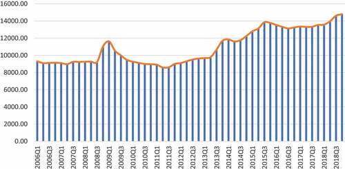
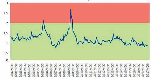
To assess stability in the financial system, Bank Indonesia uses the Financial System Stability Index that can be seen at Figure 5. The higher value of the Bank Indonesia Financial System Stability Index, the higher shock received on financial system stability (deteriorating financial system stability). Conversely, the lower value of the Bank Indonesia Financial System Stability Index, the lower shock received on financial system stability (financial system stability improved). In 2008, Bank Indonesia Financial System Stability Index tend to increase due to the effects of the global financial crisis.

Figure 5. Bank Indonesia Financial System Stability Index.

Notes: The green area is normal condition while the red one is suspected crisis.

Source: Bank Indonesia (processed)

As an effect of the global economic conditions, in 2012 Indonesia experienced net capital outflow related to the release of domestic financial assets and banking excess liquidity which was relatively high (Bank Indonesia, 2013). In 2013, the prolonged decline in commodity prices, lack of clarity over tapering off the fiscal stimulus as signaled by the Fed and uncertainty over global economic recovery have affected the domestic economic conditions. They were influenced by the trade and financial channels. Further challenges were posed by the Indonesian economy structure, which lacked the capacity to take care of pace with buoyant domestic demand. As a result, the balance of payments came under mounting emphasis, accompanied by the weakening in the exchange rate (Bank Indonesia, 2014). In 2014, the lack of certainty of monetary policy normalization by the Federal Reserve affected the Indonesian financial markets and weakened the Rupiah exchange rate (Bank Indonesia, 2015).

High dependency on outboard sources of financing also made vulnerability to fluctuations in the exchange rate, which happened in consequence of the high lack of certainty in the global financial market (Bank Indonesia, 2016a). The decline in foreign capital inflow due to an increase in the US monetary policy rate and uncertainty in the global financial market has increased the pressure on Rupiah in 2018 (Bank Indonesia, 2019). The currency depreciation was not always followed by inflation increasing rate, or on the other hand, it was not quite impacted by destabilization in financial stability.

3. Theoretical literature review

Financial stability is a condition where economy mechanisms of pricing, locating, and financial risks adjustment (credit, liquidity, market, and so forth) can be worked properly and contributed to economy performance (Schinasi, 2004). It is a condition where the financial system able to withstand financial shock without causing the cumulative process that can disrupt the allocation of savings to make investment and payment process in the economy (Padoa-Schioppa, 2002). Law No. 9 of 2016, 2016 about the prevention and treatment of the financial system crisis explains that financial stability is a condition where the financial system is effective, properly worked and able to withstand turmoil from within the country and abroad (Law No. 9 of 2016, 2016).

Minsky said that stability is destabilizing. It is similar to Schumpeter that emphasizes two phases of money role in the economy stating that in the first phase, money has been functioned as driving forces to push innovation in the production sector. When innovation has started well, there is a tendency among economy agents to become more speculative to plan their business for the future. There is cockiness that makes them not careful enough to plan their business. The consequence is money has a role to destabilize economy (phase two) when agents of economy act speculatively. Minsky said that if the economy has become stable, then its agents tend to act expansively and less cautious in debt so the situation leads to instability. So, the source of instability is a stable situation where agents of the economy tend to act speculatively. Keynes explained that their decisions were influenced by their expectations in the future, while the future itself is uncertain, so their economy actions can be regarded as natural speculative acts (Prasetyantoko, 2008).

There are several studies that use similar variables in this paper to explain financial system stability. Albulescu and Goyeau (2014) stated that stability aggregate index (afsi)_t-1, the growth of foreign currency credit to Gross Domestic Product ratio (fccgdp)_t-1, and the growth of the interbank market interest rate at three months statistically significant affects dependent variable namely stability aggregate index (afsi)_t in a negative direction. The Gross Domestic Product growth rate variable (gdpgr)_t and the growth of the Bucharest stock exchange index has significantly positive one (Albulescu & Goyeau, 2014).

Morgan and Pontines (2014) analyzed dynamic panel estimation with the dependent variable of financial stability measured by bank Z-score and bank Non-Performing Loans as an approach. The independent variables used consist of financial inclusion, logarithm of GDP per capita (lgdp_i,t), private credit by deposit money banks and other financial institutions to GDP (cgdp_i,t), liquid assets to deposits and short term funding (liq_i,t), non-FDI capital flow to GDP (nfdi_i,t), and financial openness (opns_i,t). Financial inclusion as the dependent variable in their analysis are using two measurements through Small and Medium Enterprise outstanding loans as a proportion of total outstanding loans of commercial banks (smel_i,t) and the number of Small and Medium Enterprise borrowers as a proportion of the total number of borrowers from commercial banks (smeb_i,t). In their first estimation by using measurement of variable dependent namely financial stability measured by bank Z-score and financial inclusion measured by Small and Medium Enterprise outstanding loans as a proportion of total outstanding loans of commercial banks, the result is the Gross Domestic Product per capita, liquid assets to deposits and short-term funding, financial openness and financial inclusion statistically significant affect financial stability in a positive direction, while private credit by deposit money banks and other financial institutions to Gross Domestic Product statistically significant affects financial stability in a negative direction. In the second estimation by using measurement of variable dependent namely financial stability measured by bank Z-score and financial inclusion measured by the number of Small and Medium Enterprise borrowers as a proportion of the total number of borrowers from commercial banks, the result is the Gross Domestic Product per capita, liquid assets to deposits and short-term funding and financial inclusion statistically significant affect financial stability in a positive direction, while private credit by deposit money banks and other financial institutions to Gross Domestic Product statistically significant affects financial stability in a negative direction. In the third estimation by using measurement of variable dependent namely financial stability measured by bank Non-Performing Loans and financial inclusion measured by Small and Medium Enterprise outstanding loans as a proportion of total outstanding loans of commercial banks, the result is private credit by deposit money banks and other financial institutions to GDP, and liquid assets to deposits and short term funding statistically significant affect financial stability in a positive direction, while GDP per capita, non-FDI capital flow to GDP, and financial inclusion statistically significant affect financial stability in a negative direction. In the fourth estimation by using measurement of variable dependent namely financial stability measured by bank Non-Performing Loans and financial inclusion measured by the number of Small and Medium Enterprise borrowers as a proportion of the total number of borrowers from commercial banks, the result is only financial inclusion statistically significant affects financial stability in a negative direction (Morgan & Pontines, 2014).

Kondratovs, (2012) stated that nominal effective currency exchange rate (log), real workforce effectiveness (logarithm), actual real GDP level deviation from potential real GDP to real GDP, and actual unemployment level deviation from structural unemployment level statistically significant affects dependent variable namely financial stability index in Latvia in a positive direction while ratio of foreign currency loans to nominal GDP and 3-month interbank market interest rate RIGIBOR (Riga Interbank Offered Rate) statistically significant affects dependent variable namely Latvian financial stability index in a negative direction during the 2001 year 2 quarter-2011 year 1 quarter (Kondratovs, 2012).

The research conducted by Morris (2010) demonstrated that the independent variables consist of afsi_t-1, afsi_t-2, and m2_t-1 statistically significant affects the dependent variable namely aggregate stability index in a positive direction, while the yield on 6-month treasury bill and m2 statistically significant affects the dependent variable namely aggregate stability index in a negative direction (Morris, 2010).

Albulescu (2012) revealed that economic growth and the interest rate have the significant impact toward dependent variable namely financial stability where the first has positive direction while the latter has negative one (Albulescu, 2012). Safi et al. (2021) examined that E-7 economies should concentrate on making a stable financial system, which will boost firms to adopt efficient and advance technology, and in turn, help improve the environment and decrease energy consumption (Safi, Chen et al., 2021). Gross Domestic Product, imports, exports of technological innovation and demand-related carbon emissions are co-integrated with systemic splits (Wahab, 2021). Policymakers should make financial reforms that boost and give incentives to firms that adopt eco-friendly and efficient technology to gain financial benefits (Safi, Chen et al., 2021). Financial institutions should be enabled to punish organizations that fulfilling more waste in air and water by limiting their access to easy loans (Safi, Wahab et al., 2021).

Khataybeh and Al-Tarawneh (2016) emphasize that excess reserves have a positive direction toward financial stability index and domestic credit has the significant impact toward financial stability index. These findings support the claim that monetary policy has a significant influence on financial stability through its instruments especially excess reserves (Khataybeh & Al-Tarawneh, 2016).

Dienillah and Anggraeni (2016) revealed that the correlation between financial inclusion (by using Bank Z-score indicator) and financial stability in Asia show a moderate level of relationship. Factors that significantly influence financial stability (BZS) in Asia, based on seven countries during 2007–2011, were financial stability in the previous period (AR(1)), financial inclusion (SMEL), GDP per capita (LNGDPP), non-FDI capital flow to GDP (NFDI), and ratio of current assets to deposits and short term funding (LIQ). These factors statistically significant affect financial stability in a positive direction (Dienillah & Anggraeni, 2016).

Nair and Anand (2020) stated that the central bank should contemplate a procyclical leaning against the wind. The findings from the forward-looking Taylor rule combining asset prices show the aim of price stability at the expense of output growth had retained the interest rate well above the Taylor rule originated interest rate in the recent past. An active central bank that aims asset prices besides the inflation rate and the output gap is a favored option (Nair & Anand, 2020).

Tobal and Menna (2020) concluded that monetary policy meets a more complex trade-off when dealing with financial stability in emerging market economies (EMEs) comparison with advanced economies (AEs). There are two approaches in this study. As for the first approach, in which financial stress is caused by exogenous shocks to capital flows, financial instability notices inflation and output moving in reverse directions, making it difficult to stabilize both simultaneously. As for the second approach, in which crises are endogenous, interest rate policy may be less effective at ruling in excessive credit growth, as it may stimulate additional capital inflows (Reza & Ullah, 2019).

4. Research methods

This study uses time-series quantitative data in Indonesia from 2006–2015 from the internet and literature study. Indonesian aggregate financial stability index data were compiled by chosen indicators sourced through World Bank, Bank of International Settlements, Bloomberg, and Bank Indonesia in quarterly time series during 2006–2015. Stabilization efforts can be realized through monetary policy by controlling the money supply, interest rate, and exchange rate. Money supply data in Indonesia measured by broad money in billion Rupiahs unit, collected from Bank Indonesia in the quarterly time series during that period. Interest rate data in Indonesia measured in percentage unit of BI rate and collected from Bank Indonesia in quarterly time series during the mentioned year. There was a new policy issued by Bank Indonesia related to interest rates after 2015. Exchange rate data measured through BI exchange rates calculator which based on the closing value of the transaction-average exchange rate of Rupiah per 1 USD and collected from it in quarterly time series during that period.

Financial stability (AFSI) was measured by aggregate financial stability index and it was employed a natural logarithm for analysis purposes. Aggregate Financial Stability Index was formed to achieve the purposes of this study. There are several individual indicators in the calculation of aggregate financial stability index, which generally used by kinds of literature about financial stability. Each of the individual indicators has been grouped based on four dimensions of financial stability, which is the Financial Development Index, Financial Vulnerability Index, Financial Soundness Index, and World Economic Climate Index. Financial Development Index was consisting of credit to GDP, market capitalization to GDP, interest spread and Herfindahl–Hirschman Index. Financial Vulnerability Index was consisting of inflation rate, general budget deficit/surplus (% of GDP), current account deficit/surplus (% of GDP), Real Effective Exchange Rate (REER) and loan to deposit. Financial Soundness Index was consisting of Capital Adequacy Ratio (CAR), non-performing loans to total loans, banking sector risk and return on assets. World Economic Climate Index was consisting of world economic growth, world inflation, and world economic climate. Value indicators were normalized by using the empirical normalization method. The index value of financial stability ranges from 0 to 1 where 0 means that the condition of the financial system was very unstable, while 1 means that the condition of it was very stable.

The money supply (MS) has been measured by broad money which is the sum between narrow money and quasi money. The money supply was measured in billion Rupiahs and it was employed the natural logarithm for analysis purposes. The higher the unit value is, then the higher the amount of money supply. The relationship between money supply and financial system stability can be explained by an increase in the money supply making it easier for people to take out loans and encouraging credit growth, but the growth in lender’s risk-taking behavior can reduce underwriting quality and increase the debt burden of borrowers who do not consider deleveraging externalities so it can jeopardize financial system stability (Adrian & Liang, 2016). Thus, the money supply has a negative relationship with the financial system stability.

The interest rate (IR) was measured by BI Rate, which is the reference or policy rate that has been implemented by Bank Indonesia to strengthen the framework of monetary operations. This study uses the BI Rate for analysis purposes because Bank Indonesia has replaced it with BI 7-day (Reverse) Repo Rate on 19 August 2016. The interest rate was measured in percentage and it was employed the natural logarithm for analysis purposes. The greater the unit value is then the higher the interest rate can be. The relationship between interest rates and financial system stability can be explained as in the explanation of the relationship between money supply and financial system stability. Lower interest rates make it easier for people to get loans and encourage credit growth, however, the growing risk-taking behavior of lenders can reduce the quality of underwriting and increase the debt burden of borrowers who do not consider deleveraging externalities, thereby endangering financial system stability (Adrian & Liang, 2016).

The exchange rate (ER) was measured by the transaction-average exchange rate which is the average value of buying and selling rate. Monetary policy through exchange rate control can be seen by the exchange rate indicator measured in IDR/USD, which is the price of the Indonesian Rupiah (IDR) currency measured against the United State Dollar (USD) currency, and it was employed natural logarithm for analysis purpose. When IDR currency has been appreciated then it means that IDR is stronger than USD, which reflected in the decline of the nominal currency of IDR/USD, vice versa. The direct relationship between exchange rates and financial system stability can be explained by conditions where threats to financial system stability originate from external factors, setting a floating exchange rate to prevent banks from relying excessively on external financial sources and to increase the capacity of domestic authorities to act as lenders of last resort so that financial system stability can be maintained. On the other hand, if the main threat comes from internal factors, then the policy of controlling the exchange rate through the fixed exchange rate can still be carried out to discipline domestic policy makers and to release shock through the external sector so that financial system stability can be maintained (Eichengreen, 1998).

This study is using the Stationary Stochastic Process. It was measured by Augmented Dickey-Fuller (ADF) at the same level or degree so the result was stationary data, that is the variant of it was not quite big and tend to approach its average value. If the ADF_statistic result in the stationary test was bigger than Mackinnon Critical Value then the data can be concluded as stationary because it does not contain the unit root. On the other hand, if the ADF_statistic result was smaller than Mackinnon Critical Value, then the data wasn’t stationary in the level degree. Therefore, differencing data that led to producing stationary data in an equal degree at first difference I (1) must be done by reducing it with the data from the previous period. If one of the variables was stationary at the first difference degree then all of it must be stationary at the first difference degree too (Ajija et al., 2011). The analysis of money supply, interest rate and exchange rate toward financial stability by using mathematical functions of error correction model approach written in the equation as follows:

(1) $AFSI=f\left(MS,IR,ER\right)$(1)

$AFSI$ is Indonesian aggregate financial stability index; $MS$ is Indonesian money supply, in billion Rupiahs; $IR$ is Indonesian interest rate, in percentage; and $ER$ is Indonesian exchange rate, in IDR/USD. The first procedure was estimating the long-term model, which written as follows:

(2) $LAFS{I}_t={\theta }_0+{\theta }_{1}LM{S}_t+{\theta }_{2}LI{R}_t+{\theta }_{3}LE{R}_t+u_t$(2)

where $L$ indicates natural logarithm operator; ${\theta }_0$ is intercept in equation (2)(2) $LAFS{I}_t={\theta }_0+{\theta }_{1}LM{S}_t+{\theta }_{2}LI{R}_t+{\theta }_{3}LE{R}_t+u_t$(2) ; ${\theta }_1$ is the long-run coefficient of $LM{S}_t$; ${\theta }_2$ is the long-run coefficient of $LI{R}_t$; ${\theta }_3$ is the long-run coefficient of $LE{R}_t$; $u_t$ is error term in equation (1)(1) $AFSI=f\left(MS,IR,ER\right)$(1) ; $t$ is time-series observation. When it is done, then Ordinary Least Square (OLS) residual can be calculated as follows:

(3) $\widehat{u_t}=LAFS{I}_t-\widehat{{\theta }_0}-\widehat{{\theta }_1}LM{S}_t-\widehat{{\theta }_2}LI{R}_t-\widehat{{\theta }_3}LE{R}_t$(3)

The cointegration analysis result obtained by forming residual that can be obtained through regressing independent variable toward the dependent variable in Ordinary Least Square. That residual has to stationary in level degree so it has cointegration. It can be done through the Dickey-Fuller Stationarity test by seeing the significant t-statistic value toward critical value (Basuki, 2015).

(4) $\mathrm{\Delta }{u}_t={\delta }_1{u}_{t-1}+v_t$(4)

where ${\delta }_1$ is the coefficient of $u_{t-1}$; $u_{t-1}$ is the lagged value of the error term in equation (1)(1) $AFSI=f\left(MS,IR,ER\right)$(1) ; and $v_t$ is the error term in equation (4)(4) $\mathrm{\Delta }{u}_t={\delta }_1{u}_{t-1}+v_t$(4) .

The estimation result of the Error Correction Model shows compatibility between long- and short-term relations that can be corrected. It is also can be used to calculate how far the short term elasticity in independent variables (Ajija et al., 2011). The equation of ECM in this study can be seen as follows (Gujarati & Porter, 2009):

(5) $\mathrm{\Delta }LAFS{I}_t={\psi }_0+{\psi }_1\mathrm{\Delta }LM{S}_t+{\psi }_2\mathrm{\Delta }LI{R}_t+{\psi }_3\mathrm{\Delta }LE{R}_t+{\psi }_4{u}_{t-1}+{\epsilon }_t$(5)

where ${\psi }_0$ is intercept in equation (5)(5) $\mathrm{\Delta }LAFS{I}_t={\psi }_0+{\psi }_1\mathrm{\Delta }LM{S}_t+{\psi }_2\mathrm{\Delta }LI{R}_t+{\psi }_3\mathrm{\Delta }LE{R}_t+{\psi }_4{u}_{t-1}+{\epsilon }_t$(5) ; ${\psi }_1$ is the short-run coefficient of $\mathrm{\Delta }LM{S}_t$; ${\psi }_2$ is the short-run coefficient of $\mathrm{\Delta }LI{R}_t$; ${\psi }_3$ is the short-run coefficient of $\mathrm{\Delta }LE{R}_t$; ${\psi }_4$ is the discrepancy of AFSI—from the robust estimation—to achieve equilibrium; ${\epsilon }_t$ is the White noise error term. Ordinary Least Square has been used because this equation has variables that located only in level degree, standard hypothesis test used t-ratio, and error term diagnostic test has appropriate. The adjustment coefficient ${\psi }_4$ has to be negative.

5. Results and discussion

Table 1 showed the descriptive statistics of the variables examined in this study. The results demonstrated the mean, median, maximum, minimum, standard deviation, skewness and kurtosis for each variable.

Table 1. Descriptive statistics

	AFSI	MS	IR	ER
Mean	0.531750	2,593,015.	7.660750	10,136.81
Median	0.525000	2,406,014.	7.500000	9305.770
Maximum	0.620000	4,481,401.	12.75000	13,850.88
Minimum	0.370000	1,197,153.	5.750000	8590.370
Std. Dev.	0.059910	1,021,308.	1.744816	1490.019
Skewness	−0.879909	0.358870	1.440930	1.154985
Kurtosis	3.743571	1.853371	4.812609	3.095502

Furthermore, Stationary Stochastic Process was measured by Augmented Dickey-Fuller (ADF) at the same level or degree so the result was stationary data, that is the variant of it was not quite big and tend to approach its average value. If the ADF_statistic result in the stationary test was smaller than Mackinnon Critical Value, then the data wasn’t stationary in the level degree. Therefore, differencing data that led to producing stationary data in an equal degree at first difference I (1) must be done and so on until all variables have stationary at the degree the same (Ajija et al., 2011).

Based on Table 2, LAFSI, LMS, and LER are not stationary in Level or I(0). It was caused by the probability value of LAFSI, LMS, and LER was bigger than $\alpha =5\mathrm{\%}$. It can be calculated by seeing its Critical Value (5% level) that smaller than the t-statistic ADF Test. Therefore, this test continues to calculate the integration degree test by looking at what difference level all variables are stationary. Table 3 is the estimation results of the difference stationary process at the first difference.

Table 2. Estimation result of the stationary stochastic process at level

Variable	Prob. ADF Test	t-Statistic ADF Test	Critical Value (5% level)
LAFSI	0.2156	−2.1827	−2.9411
LMS	0.6135	−1.3140	−2.9390
LIR	0.0200	−3.3377	−2.9411
LER	0.8400	−0.6789	−2.9411

Table 3. Estimation result of the difference stationary process at first difference

Variable	Prob. ADF Test	t-Statistic ADF Test	Critical Value (5% level)
LAFSI	0.0008	−4.5290	−2.9411
LMS	0.0000	−6.2153	−2.9411
LIR	0.0047	−3.9155	−2.9434
LER	0.0014	−4.3555	−2.9411

Based on Table 3, all variables have been stationary at first difference or I(1). It was caused by all of the probability value in all variables that were smaller than $\alpha =5\mathrm{\%}$. It can be concluded also by seeing the Critical Value (5% level) which has a bigger value than the t-statistic ADF Test. So, all variables were stationary at first difference or I(1) at $\alpha =5\mathrm{\%}$.

The first procedure was estimating the long-term model. The long-run model in this study can be seen at Table 4.

Table 4. Estimation result of the long-run model: dependent variable is LAFSI

Variable	Coefficient	t-Statistic	Prob.
LMS	0.2817	2.4620	0.0187**
LIR	0.4161	2.4763	0.0181**
LER	−0.3292	−1.2485	0.2199
C	−2.5817	−2.0905	0.0437

Notes: *) significant at $\alpha =1\mathrm{\%}$; **) significant at $\alpha =5\mathrm{\%}$; ***) significant at $\alpha =10\mathrm{\%}$ level of confident

Table 4 shows the estimation result of the long-run model for this research can be seen as follows:

(6) $LAFS{I}_t=-2.5817+0.2817LM{S}_t+0.4161LI{R}_t-0.3292LE{R}_t+u_t$(6)

Statistically, the money supply has a significant relationship toward financial stability. Money supply has positive direction at $\alpha =5\mathrm{\%}$, ceteris paribus. This positive direction shows that increasing the money supply will also enhance financial stability in the long term and vice versa. This finding is in line with Morris (2010) although the direction has a different result.

The same things happen at the interest rate. Interest rate has a significant relationship toward financial stability. Interest rate has positive direction at $\alpha =5\mathrm{\%}$, ceteris paribus. Its increase will enhance financial stability in the long term and vice versa. The interest rate significance finding is in line with Albulescu (2012) although the direction has a negative relationship toward financial stability.

One percent of increasing money supply means 0.2817 percent Indonesian financial stability enhancement and one percent of increasing interest rate can increase 0.4161 percent Indonesian financial stability in the long term. The result of the long-term estimation model was supported also by the result of the cointegration analysis. The estimated critical value for the cointegration test can be seen as follows (MacKinnon, 2010):

(7) ${\beta }_{\mathrm{\infty }}+\frac{{\beta }_1}{T}+\frac{{\beta }_2}{T^2}+\frac{{\beta }_3}{T^3}$(7)

$=-4.119+\frac{-11.892}{40}+\frac{-19.031}{1600}+\frac{77.332}{64000}$

$=-4.119-0.297-0,012+0.001=-4.427$

where ${\beta }_{\mathrm{\infty }}$ is estimated asymptotic critical values (with estimated standard errors in parentheses); ${\beta }_1$ is coefficient on T⁻¹ in response surface regression; ${\beta }_2$ is coefficient on T⁻² in response surface regression; ${\beta }_3$ is coefficient on T⁻³ in response surface regression; $T$ is the sample size. After doing the test of cointegration to test the resulting residual, it is found that the residual series from (6) is stationary at Level degree or I(0). It was caused by its probability value (0.0130) was smaller than $\alpha =5\mathrm{\%}$. It can be concluded that the data has been cointegrated at 5% level.¹ It shows a balanced relationship between the research variables has been proven statistically as indicated by the long-term residual that has been stationary at level degree or I(0).

Based on Table 5, Error Correction Model for this research can be seen as follows:

(8) $\mathrm{\Delta }LAFS{I}_t=0.0259-0.9391\mathrm{\Delta }LM{S}_t-0.4149\mathrm{\Delta }LI{R}_t+0.1437\mathrm{\Delta }LE{R}_t-0.2400u_{t-1}+{\epsilon }_t$(8)

Table 5. Estimation result of the error correction model: dependent variable is ∆LAFSI

Variable	Coefficient	t-Statistic	Prob.
D(LMS)	−0.9391	−1.4283	0.1623
D(LIR)	−0.4149	−2.3356	0.0256**
D(LER)	0.1437	0.5288	0.6004
RESIDUAL(−1)	−0.2400	−2.5063	0.0171**
C	0.0259	1.1150	0.2727

Notes: *) significant at $\alpha =1\mathrm{\%}$; **) significant at $\alpha =5\mathrm{\%}$; ***) significant at $\alpha =10\mathrm{\%}$ level of confident

It shows that the coefficient of residual series in that model has significant at $\alpha =5\mathrm{\%}$ and has a negative direction to financial stability (AFSI) estimation which Error Correction Model in short term can be proven by significant and negative $u_{t-1}$.

The estimation result describes that short-term change in interest rate has negative direction and significant at $\alpha =5\mathrm{\%}$ toward financial stability, ceteris paribus. This finding in line with Albulescu (2012) that the interest rate has significant negative direction. The negative direction shows that increasing interest rate can be destabilizing financial stability in short term model and vice versa. Based on the significant value of $u_{t-1}$, the difference between financial stability and its balance value will be adjusted by lag. The coefficient of residual series by −0.2400 means that the difference between financial stability with its balance value as big as 24 percent and will be adjusted in four times period. The influence of interest rate toward financial stability in the short term shows that one percent of increasing interest rate can be destabilizing financial stability by 0.4149 percent.

6. Conclusion and policy implication

This study has proven the main factors of monetary policy in maintaining Indonesian financial stability by drawing the conclusion that money supply and interest rate statistically significant affects financial stability in the long-run at $\alpha =5\mathrm{\%}$ in a positive direction, ceteris paribus. That positivity shows increasing money supply means financial stability enhancement in the long-run and vice versa. It has the same effects when increasing interest rate mean financial stability will be more stable in the long term and vice versa. One percent of increasing money supply can enhance 0.2817 percent of Indonesian financial stability in the long-run, and then one percent of increasing interest rate can enhance 0.4161 percent of Indonesian financial stability in the long-run.

Residual has been stationary at level degree or I(0) so it can be said that the data in this research were cointegrated and the short term model of ECM can be proven statistically through its significant value and negative direction. Short-term changing of interest rate has negative direction and significant at $\alpha =5\mathrm{\%}$ toward financial stability, ceteris paribus. This negative direction shows that interest rate enhancement will be destabilizing financial stability in the short-run model, vice versa. The influence of interest rate toward financial stability in the short term shows that one percent of increasing interest rate can be destabilizing financial stability by 0.4149 percent. The difference between financial stability with its balance is 24 percent, will be adjusted in four times period.

Empirically, monetary policy is necessary to control financial stability in Indonesia. Bank Indonesia can use the interest rate instrument to maintain financial stability. Empirically, the enhancement of interest rate can stabilize financial stability in Indonesia and vice versa. The enhancement of interest rate can lower speculative acts so market agents can be more careful to manage its finance, especially in high-risk acts. Risk-averse behavior in the capital market can increase Indonesian financial liquidity through the enhancement of interest rate so the risk of drought in it is getting smaller. It will maintain the financial system more stable. The enhancement of interest rate can increase Indonesian financial stability within four times period responsively, with one percent of increasing interest rate can increase 0.4161 percent Indonesian financial stability.

Money supply enhancement can stabilize the Indonesian financial system in the long-run. That enhancement, in the long-run, will have a positive expectation of stable inflation. Stable inflation can increase market and investor confidence to drive the real sector in Indonesia. The good real sector investment climate in the long term will benefit Indonesia. The government needs to pay attention to this thing, so in the long-run, the investor will not withdraw their fund abroad when the development period of real sectors is commencing. Investor fund withdrawal at the same time massively will shock the economy within the country so that the risk of crisis is getting bigger. Empirically, one percent of increasing money supply can enhance 0.2817 percent of Indonesian financial stability in the long-run.

7. Limitations

The limitation of this research lies in its data access availability. The data publication of Indonesian financial stability in Bank Indonesia is very limited. Financial stability data series are not published on the Bank Indonesia website. It only delivered Indonesian financial stability charts routinely published in the Financial Stability Review since 2014. Therefore, the authors try to calculate the Indonesian financial stability index with chosen indicators that have been used by previous studies. Some limitations were also found when the authors tried to choose selected indicators in compiling Indonesian aggregate financial stability index, such as the availability of data for certain individual indicators; and some other indicators that has availability of the data but it has the different type of periods so that it is necessary to adjust the data interpolation. Those individual indicators are Interest Spread, Herfindahl—Hirschman Index, General Budget Deficit/Surplus (% of GDP), and World Economic Growth which usually served annually so that the data interpolation is done into quarterly.

This research also has limitations in the time period that took data only from the 2006–2015 period so it cannot be used as the source to explain how far the monetary policy influences financial stability before, when, and after the financial crisis struck Indonesia in 1997/1998. Furthermore, it is also doesn’t have an explanation regarding how was the condition of the economic system and its influence on financial stability in Indonesia during 2016–2017 because Bank Indonesia has replaced BI Rate with BI 7-day (Reverse) Repo Rate on 19 August 2016.

8. Future guidelines

To achieve a more comprehensive result in the future, by some limitations of the method in this study, it can be done some developments. Financial stability is not influenced by monetary policy alone. Other policy variables can be included in this study to get a complete understanding of how the policy mix can influence financial stability in Indonesia. Therefore, other policy variables are a good addition to create a new model that can explain how far policy mix can control financial stability in Indonesia and also it can be used as policy decision material in the future.

Acknowledgements

We gratefully acknowledge funding provided by Bank Indonesia Institute (BINS) for the 2018 thesis research funding (Bantuan Penelitian/Banlit Program) in collaboration with the Faculty of Economics and Business Diponegoro University.

Disclosure statement

No potential conflict of interest was reported by the author(s).

Additional information

Funding

This work was supported by Bank Indonesia Institute (BINS).

Notes on contributors

Afaqa Hudaya

Afaqa Hudaya earned his bachelor’s degree in Economics and Development Studies from Syarif Hidayatullah State Islamic University in Jakarta and completed his master’s degree in Economics from Diponegoro University with cum laude predicate. Afaqa was a recipient of the 2018 thesis research funding from the Bank of Indonesia Institute. His thesis analyzed how the monetary policy affected financial stability in Indonesia between 2006 and 2015. Afaqa also had a number of research experiences while completing his master’s degree. He assisted numerous research projects from various institutions, including the Central Bank of Indonesia, Bank Jateng, General Secretariat Research Center, and Expertise Agency at the House of Representatives of the Republic of Indonesia, Ministry of Investment of the Republic of Indonesia/ Indonesia Investment Coordinating Board and so forth.

Firmansyah Firmansyah

FirmansyahFirmansyah is the vice dean and senior lecturer in the Faculty of Economics and Business, Universitas Diponegoro, Semarang, Indonesia. He received his bachelor’s and master’s degrees in economics from Gadjah Mada University, Yogyakarta, Indonesia. He obtained his Ph.D. from Curtin University, Perth, Australia. His study interests are microeconomics, econometrics, and industrial economy.

References

- Adrian, T., & Liang, J. N. (2016). Monetary policy, financial conditions, and financial stability. Federal Reserve Bank of New York, Staff Reports, no. 690. https://www.newyorkfed.org/medialibrary/media/research/staff_reports/sr690.pdf
- Ajija, S. R., Sari, D. W., Setianto, R. H., & Primanti, M. R. (2011). Cara cerdas menguasai Eviews. Salemba Empat.
- Albulescu, C. T. (2012). Financial stability, monetary policy and budgetary coordination in EMU. Theoretical & Applied Economics, 19(8), 85–17. http://store.ectap.ro/articole/764.pdf
- Albulescu, C. T., & Goyeau, D. (2014). Assessing and forecasting romanian financial system’s stability using an aggregate index. https://www.researchgate.net/publication/228360426_Assessing_and_Forecasting_Romanian_Financial_System’s_Stability_Using_an_Aggregate_Index
- Bank Indonesia. (2007). Laporan tahunan bank Indonesia 2006. https://www.bi.go.id/id/publikasi/laporan-tahunan/bi/Pages/ltbi2006.aspx
- Bank Indonesia. (2008). Laporan Tahunan Bank Indonesia 2007. https://www.bi.go.id/id/publikasi/laporan-tahunan/bi/Pages/lktbi_07.aspx
- Bank Indonesia. (2009). Laporan Tahunan Bank Indonesia 2008. https://www.bi.go.id/id/publikasi/laporan-tahunan/bi/Pages/ltbi_2008.aspx
- Bank Indonesia. (2010). Laporan Tahunan Bank Indonesia 2009. https://www.bi.go.id/id/publikasi/laporan/Pages/ltbi_09.aspx
- Bank Indonesia. (2013). Laporan Tahunan Bank Indonesia Tahun 2012: https://www.bi.go.id/id/publikasi/laporan-tahunan/bi/Pages/LaporanTahunanBankIndonesiaTahun2012.aspx
- Bank Indonesia. (2014). Laporan Tahunan Bank Indonesia 2013. https://www.bi.go.id/id/publikasi/laporan-tahunan/bi/Pages/LTKBI-2013.aspx
- Bank Indonesia. (2015). Laporan Tahunan Bank Indonesia 2014. https://www.bi.go.id/id/publikasi/laporan-tahunan/bi/Pages/LKTBI-2014a.aspx
- Bank Indonesia. (2016a). Laporan Tahunan Bank Indonesia 2015: https://www.bi.go.id/id/publikasi/laporan-tahunan/bi/Pages/LKTBI-2015.aspx
- Bank Indonesia. (2016b). Mengupas Kebijakan Makroprudensial.
- Bank Indonesia. (2018a). Definisi stabilitas sistem keuangan. https://www.bi.go.id/id/perbankan/ssk/ikhtisar/definisi/Contents/Default.aspx (Accessed: 23 June 2018)
- Bank Indonesia. (2018b). Laporan Tahunan Bank Indonesia 2017. https://www.bi.go.id/id/publikasi/laporan-tahunan/bi/Pages/LKTBI-2017.aspx
- Bank Indonesia. (2018c). Pentingnya stabilitas sistem keuangan. https://www.bi.go.id/id/perbankan/ssk/ikhtisar/pentingnya/Contents/Default.aspx. 23 June 2018)
- Bank Indonesia. (2019). Laporan Tahun Bank Indonesia 2018. https://www.bi.go.id/id/publikasi/laporan-tahunan/bi/Pages/LKTBI-2018.aspx
- Basuki, A. T. (2015). Regresi Model PAM, ECM, dan data panel dengan eviews 7. Andi Offset.
- Dhal, S., Kumar, P., & Ansari, J. (2011). Financial stability, economic growth, inflation and monetary policy linkages in India: An empirical reflection. Reserve Bank of India Occasional Papers, 32(3), 1–35. https://rbidocs.rbi.org.in/rdocs/content/pdfs/1afstab100114.pdf
- Dienillah, A. A., & Anggraeni, L. (2016). Dampak inklusi keuangan terhadap stabilitas sistem keuangan di Asia. Buletin Ekonomi Moneter Dan Perbankan, 18(4), 409–430. https://doi.org/10.21098/bemp.v18i4.574
- Eichengreen, B. (1998). Exchange rate stability and financial stability. Open Economies Review, 9(1), 569–608. https://doi.org/10.1023/A:1008373022226
- Gujarati, D. N., & Porter, D. C. (2009). Basic Econometrics (5th) ed.). McGraw-Hill/Irwin.
- Khataybeh, M., & Al-Tarawneh, A. (2016). Impact of monetary policy on financial stability evidence from Jordan. Dirasat, Administrative Sciences, 43(1), 301–313. https://doi.org/10.12816/0028464
- Kondratovs, K. (2012). Modelling financial stability index for Latvian financial system. Regional Formation and Development Studies, 8(3), 118–129. https://doi.org/10.15181/rfds.v7i2.2368
- Law No. 9 of 2016. (2016). The prevention and handling of financial system crisis. https://jdih.kemenkeu.go.id/fullText/2016/9TAHUN2016UU.pdf
- MacKinnon, J. G. (2010). Critical values for cointegration tests. Queen’s Economics Department Working Paper, No. 1227, Queen’s University, Department of Economics, Kingston (Ontario). https://www.econstor.eu/bitstream/10419/67744/1/616664753.pdf
- Morgan, P., & Pontines, V. (2014). Financial stability and financial inclusion. ADBI Working Paper Series, No. 488, Asian Development Bank Institute (ADBI), Tokyo. https://www.adb.org/sites/default/files/publication/156343/adbi-wp488.pdf.
- Morris, V. C. (2010). Measuring and forecasting financial stability: The composition of an aggregate financial stability index for Jamaica. Bank of Jamaica, Research Papers 2010, 1–19. https://www.boj.org.jm/uploads/pdf/papers_pamphlets/papers_pamphlets_Measuring_and_Forecasting_Financial_Stability__The_Composition_of_an_Aggregate_Financial_Stability_Index_for_Jamaica.pdf
- Nair, A. R., & Anand, B. (2020). Monetary policy and financial stability: Should central bank lean against the wind? Central Bank Review, 20(3), 133–142. https://doi.org/10.1016/j.cbrev.2020.03.006
- Padoa-Schioppa, T. (2002). Central banks and financial stability: Exploring a land in between. second ECB Central banking conference, “The transformation of the European financial system”, Frankfurt am Main, 25 October 2002. https://www.ecb.europa.eu/events/pdf/conferences/tps.pdf.
- Pattawe, A., Abdullah, M. I., Karim, F., Kahar, A., Din, M., Zahra, F., Furqan, A. C., & Dharma, D. M. A. (2022). Improving regional financial management through administration of regional property and financial reporting on regional assets. Research Horizon, 2(1), 283–294. https://doi.org/10.54518/rh.2.1.2022.283-294
- Prasetyantoko, A. (2008). Bencana Finansial: Stabilitas Sebagai Barang Publik. Penerbit Buku Kompas.
- Rahim, S., Murshed, M., Umarbeyli, S., Kirikkaleli, D., Ahmad, M., Tufail, M., & Wahab, S. (2021). Do natural resources abundance and human capital development promote economic growth? A study on the resource curse hypothesis in Next Eleven countries. Resources, Environment and Sustainability, 4, 100018. https://doi.org/10.1016/j.resenv.2021.100018
- Reza, M., & Ullah, S. (2019). Financial reporting quality of the manufacturing firms listed in Indonesian Stock Exchange. Arthatama, 3(1), 37–54. https://arthatamajournal.co.id/index.php/home/article/view/27
- Safi, A., Chen, Y., Wahab, S., Ali, S., Yi, X., & Imran, M. (2021). Financial instability and consumption-based carbon emission in E-7 countries: The role of trade and economic growth. Sustainable Production and Consumption, 27, 383–391. https://doi.org/10.1016/j.spc.2020.10.034
- Safi, A., Wahab, S., Zeb, F., Amin, M., & Chen, Y. (2021). Does financial stability and renewable energy promote sustainable environment in G-7 Countries? The role of income and international trade. Environmental Science and Pollution Research, 28(34), 47628–47640. https://doi.org/10.1007/s11356-021-13991-7
- Schinasi, G. J. (2004). Defining Financial Stability. IMF Working Papers, 2004(187). International Monetary Fund, Washington, DC. https://doi.org/10.5089/9781451859546.001.
- Tobal, M., & Menna, L. (2020). Monetary policy and financial stability in emerging market economies. Latin American Journal of Central Banking, 1(1–4), 100017. https://doi.org/10.1016/j.latcb.2020.100017
- Wahab, S. (2021). Does technological innovation limit trade-adjusted carbon emissions? Environmental Science and Pollution Research, 28(28), 38043–38053. https://doi.org/10.1007/s11356-021-13345-3
- Wahab, S., Imran, M., Safi, A., Wahab, Z., & Kirikkaleli, D. (2022). Role of financial stability, technological innovation, and renewable energy in achieving sustainable development goals in BRICS countries. Environmental Science and Pollution Research, 1–12. https://doi.org/10.1007/s11356-022-18810-1
- Wahab, S., Zhang, X., Safi, A., Wahab, Z., & Amin, M. (2021). Does energy productivity and technological innovation limit trade-adjusted carbon emissions? Economic Research-Ekonomska Istraživanja, 34(1), 1896–1912. https://doi.org/10.1080/1331677X.2020.1860111
- Warjiyo, P., & Juhro, S. M. (2016). Kebijakan bank sentral: teori dan praktik. RajaGrafindo Persada.