Fiscal capacity and public health expenditure in Zimbabwe

Abstract

Public healthcare financing is important for achieving one of the 2030 Sustainable Development Goals (SDGs), the goal of healthy living and well-being (SDG3). Understanding the impact of fiscal capacity on public healthcare financing helps in assessing the government’s commitment towards attaining SDG3. The study sought to investigate the relationship between fiscal capacity and public health expenditure in Zimbabwe. An Autoregressive Distributed Lag (ARDL) model was estimated using annual time series data for the period 1980–2017. The results of the ARDL model were validated using the Fully Modified Ordinary Least Squares (FMOLS) and Canonical Cointegrating Regression (CCR) methods. The study found that fiscal capacity (measured as the ratio of tax revenue to GDP) impacted positively on public health expenditure. The results suggest that following an improvement in resources, the government prioritised the health sector. The study recommends that the government continues to prioritise health in the national budget to enhance the country’s achievement of SDG3.

Keywords:

• public health expenditure
• fiscal capacity
• tax revenue
• gross domestic product
• ARDL model
• Zimbabwe

1. Introduction

Globally, the government plays a key role in the financing of social services such as healthcare. However, the extent of government healthcare financing relative to other financing mechanisms generally varies across nations. In some countries, private health insurance plays a significant role, while in other nations Out of Pocket (OOP) health expenses are substantial. Achieving Universal Health Coverage (UHC), an important target under goal 3 of the 2030 Sustainable Development Goals (SDGs), is generally possible in the presence of effective public prepayment arrangements for healthcare such as government tax financing. UHC is aimed at ensuring access to needed healthcare for all without experiencing financial hardship (United Nations 2015). Jakovljevic, Liu et al. (2021) argue that achieving UHC is a challenge in low- and middle-income countries (LMICs) as well as in some of the world’s richest nations. The authors further argue that increased healthcare financing alone may not make the road to UHC clear—other measures such as dealing with corruption and improving health expenditure efficiency are necessary.

In Zimbabwe, government tax financing has been the main healthcare financing model since independence in 1980. However, fiscal allocations to health have generally fallen short of the Ministry’s requirements and the 15% of the national budget specified in the Abuja (2001) Declaration. The Ministry of Finance and Economic Development (Ministry of Finance and Economic Development (MoFED), 2019) acknowledges that the Abuja target has largely remained elusive for Zimbabwe. This study sought to investigate the impact of fiscal capacity on public health expenditure (PHE) in Zimbabwe. To achieve this objective, an Autoregressive Distributed Lag (ARDL) model was estimated using annual time series data for the period 1980–2017. The results of the ARDL model were validated using the Fully Modified Ordinary Least Squares (FMOLS) and Canonical Cointegrating Regression (CCR) methods.

An understanding of the relationship between fiscal capacity and PHE helps to evaluate the extent to which the government prioritised the health sector despite facing fiscal challenges. In some countries, despite substantial increases in fiscal capacity, spending on healthcare does not improve; instead, the additional resources are directed towards military expenditure (Jakovljevic, Ranabhat et al., 2021; Murshed et al., 2017). Murshed et al. (2017) and Murshed et al. (2020) observe that very few studies have investigated the impact of fiscal capacity on social expenditure in developing countries. With regards to the relationship between fiscal capacity and PHE in Zimbabwe, three studies (Xu et al., 2011; Micah et al., 2019; Murshed et al., 2017), have included Zimbabwe in panel regressions in this study area. Unlike these studies, which used panel data on many countries, this research focuses on a single country (Zimbabwe) and uses yearly time series data covering a much longer period (1980–2017). Whilst panel data has several advantages over time series data (for example, fewer problems of multicollinearity, increased variability, highly informative data, efficiency; Baltagi, 2008; Hsiao, 2007), it has the limitation that the researcher cannot easily suggest country-specific recommendations from panel regression results.

Moreover, no known study has applied the relatively novel methodology, the bounds approach to cointegration proposed by Pesaran et al. (2001), to investigate the effect of fiscal capacity on PHE in Zimbabwe, nor to analyse the determinants of PHE in the country. Dhoro et al. (2011) conducted a Zimbabwean study on the determinants of PHE, but the study applied the Engle-Granger cointegration approach and did not consider the fiscal capacity variable. The application of Pesaran et al. (2001)’s bounds approach has a couple of advantages—it deals with the endogeneity problem, super-consistent estimates are obtained even for a small sample size, and it can be applied on regressors integrated of order zero, order one, or a combination of these (Menegaki, 2019; Murthy & Okunade, 2016; Narayan, 2005).

The rest of the paper is organised as follows: trends in fiscal capacity and PHE are presented in section 2. Section 3 provides a literature review (both theoretical and empirical) on the issue under investigation, while section 4 presents the methodology. The results of the study are presented in section 5, and subsequently discussed in section 6. The last section concludes the paper.

2. Trends in fiscal capacity and public health expenditure in Zimbabwe

As shown in Figure 1, during the period 1980–2017, significant fluctuations have been witnessed in tax revenue (as a share of GDP). It stayed above 15% for the greater part of the period (1980–2004), with the highest values of close to 35% being observed in 1998 and 2004. During the peak of Zimbabwe’s economic crisis (2007–2008), tax revenues fell to below 5% of GDP. It was also during these years when the country’s official inflation rate reached record levels of over 230 million percent (Hanke & Kwok, 2009). Unlike tax revenue, PHE (as a share of GDP) generally remained stable throughout the period; it has largely stayed below 5% of GDP. Like tax revenue, PHE was at its lowest (less than 1% of GDP) during the years 2007 and 2008. Other authors described the period 1997–2008 as a phase of “growth reversal”—Zimbabwe experienced a severe crisis characterised by deindustrialisation, high unemployment, rising poverty levels, high outmigration of people, among other challenges (Madebwe & Madebwe, 2017; Manjokoto & Ranga, 2017; Nyazema, 2010).

Figure 1. Trends in fiscal capacity and public health expenditure.

Sources: Author based on Dhliwayo (2001), Munyuki and Jasi (2009), and Mansour (2014); COMESA (Common Market for Eastern and Southern Africa (COMESA), 2020, International Monetary Fund (IMF; 2021), and World Bank (WB; 2021).

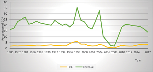
After experiencing the severe economic crisis (late 1990s to 2008), there were significant changes in Zimbabwe’s political and economic landscape in 2009. First, a Government of National Unity (GNU) was formed, thus reducing the political tensions that had existed in the country for more than a decade. Second, the multiple currency system was embraced, and this helped to end the hyperinflation that was being experienced during the use of the local currency. As depicted in Figure 1, tax revenue and PHE levels bounced to the historical averages of 19% and 2.5% of GDP, respectively.

3. Literature review

In this section, the theoretical literature on public expenditure and the empirical literature on the determinants of public health expenditure is reviewed. First is a discussion of the public finance theories, and then a review of the key drivers of public health expenditure. The theories of public finance discussed are Wagner (1883)’s Law of increasing state activity, Peacock and Wiseman (1961)’s Displacement theory, and the Revenue-Spend hypothesis (Friedman, 1978).

3.1. Theoretical literature review

3.1.1. Wagner’s Law of increasing state activity

Propounded in 1883 by a German economist, Adolph Wagner, the law of increasing state activity hypothesises a rise in public spending as the government’s economic, legal, social, and political involvement expands. The rise in expenditure occurs at both central and local governments. According to Jibir and Aluthge (2019), Azolibe et al. (2020), and Gbaka et al. (2021), and Olayiwola, Bakare-Aremu and Abiodun (Olayiwola et al., 2021) the possible avenues leading to this phenomenon are economic development, population growth, and industrialisation. Economic development, manifested in GDP growth per capita, entails increased public revenues and hence expansion of state activities. Thus, state activities are endogenously determined by economic development, that is, increases in per capita GDP are associated with rising public revenues which in turn lead to increases in government spending. In summary, the Wagnerian hypothesis postulates a positive relationship between the size of an economy and the state’s involvement/ functions/ activities, and in turn, government expenditure.

3.1.2. The Revenue-Spend hypothesis

Also known as the Tax-Spend hypothesis, the theory was proposed by Friedman (1978). The main argument behind the theory is that government revenue drives public expenditure, that is, a positive relationship exists between taxes and public spending (Aladejare, 2019; Jibir & Aluthge, 2019; Jaén-García 2020; Afonso et al., 2021; Linhares et al., 2021). It follows that when the government increases taxes, its expenditure rises too, thereby creating fiscal imbalances (Aladejare, 2019). From Friedman (1978)’s viewpoint, tax limitation laws (citizens deciding a limit on the government’s budget) are necessary for curbing increased government spending. Once the people decide the government’s budget, it becomes the responsibility of those elected in public offices to decide how best to make use of the limited revenue in the face of competing obligations. Unlike Friedman (1978)’s view of a positive impact of taxes on expenditure, Buchanan and Wagner (1978) predict a negative relationship. The authors argue that when taxes are reduced, the public perceives a reduction in the cost of running government programmes, hence they demand new public programmes to be instituted. Once the government gives in to such demands, public expenditure inevitably outpaces public revenue, resulting in budget deficits (Aladejare, 2019).

3.1.3. The Displacement theory

Unlike the Revenue-Spend Hypothesis which posits that taxes lead to spending, Peacock and Wiseman (1961)’s Displacement Theory (also called the Spend-Revenue or Spend-Tax Hypothesis) postulates that a temporary increase in government expenditure creates a permanent need for higher taxes/ revenues (Azolibe et al., 2020; Gbaka et al., 2021; Linhares et al. 2021). The temporary increase in public spending could be due to economic, social, or political instability, for example, health crises and wars. It is argued that when a nation is faced with such difficult circumstances, citizens could be more willing to pay taxes in order to improve the situation. However, even after the crisis has been overcome, the government will encourage taxpayers to be tolerant of the new high taxes, hence a permanent displacement from the tax level in the past (the displacement effect). Put differently, the Spend-Tax Hypothesis argues that changes in taxes are driven by changes in public expenditures. It follows that expenditure takes precedence over revenues, thus increasing the likelihood of escalating budget deficits, whose burden future generations will have to shoulder.

3.2. Empirical literature review

3.2.1. Relationship between fiscal capacity and social expenditure

Different proxies of fiscal capacity have been used by studies that included the variable in empirical analysis. One proxy that has been widely adopted is the ratio of total government tax revenue to GDP, a measure popularised by Besley and Persson (2013). Researchers who have utilised the proxy include Baskaran and Bigsten (2013), Chowdhury and Murshed (2016), Rota (2016), Behera and Dash (2019), (Micah et al., 2019), Ricciuti, Savoia and Sen (2019), and Sfakianakis et al. (2021). Other proxies of fiscal capacity utilised are a state’s total revenue (Hooda, 2016) and the ratio of total government revenue to GDP (Murshed et al., 2017). Yet other studies have embraced total government expenditure as a share of GDP (Xu et al. 2011; Micah et al., 2019), or the share of general government expenditure to GDP (Behera & Dash, 2020; Sfakianakis et al. 2021). Generally, fiscal capacity has been found to impact positively on PHE (Xu et al. 2011; Behera & Dash, 2019; Hooda, 2016; Micah et al., 2019; Murshed et al., 2020).

3.2.2. Other determinants of public health expenditure

Besides fiscal capacity, several factors influence PHE. Among them is income, population structure, urbanization, and external debt. The effect of these factors on health expenditure is discussed in this section.

Newhouse (1977) did a pioneering study on the relationship between income and health expenditure. The study was conducted on a sample of 13 developed countries, most of them from the European region. Newhouse (1977) observed that income alone (measured as GDP per capita) explained at least 90 % of the changes in a country’s medical-care expenditure. The results also showed that the income elasticity of health expenditure for the sampled countries was greater than one, implying that medical care was a luxury product. Following the seminal work of Newhouse (1977), several studies that included non-income variables and employed different methodologies have been conducted, and mixed results on medical care being a necessity or luxury were obtained. However, most contemporary studies have established that healthcare is a need rather than a luxury—an income elasticity less than unity has generally been obtained regardless of whether total or PHE was being considered (Abbas & Hiemenz, 2013; Baltagi & Moscone, 2010; Barkat et al., 2019; Chaabouni & Abednnadher, 2014; Hooda, 2016; Khan & Husnain, 2019; Micah et al., 2019; Murthy & Okunade, 2016). Moreover, the empirical findings have generally confirmed a positive relationship between income and health expenditure, suggesting that healthcare is a normal good.

The population structure of a country is another factor that influence healthcare expenditure. In particular, a rise in the proportion of the elderly population (people older than 65 years or 75 years) relative to the total population, tends to be associated with an increase in health costs. This is partly because the frequency of illness among the elderly is high and so is the duration of ill-health and in turn the treatment costs (Morris et al., 2012). Although some scholars have questioned the relevance of population ageing in explaining health expenditure (Hartwig, 2008; Zweifel et al., 1999), studies conducted recently have confirmed that the variable continues to be a significant predictor of increased health expenditure (Xu et al. 2011; Chaabouni & Abednnadher, 2014; Murthy & Okunade, 2016; Barkat et al., 2019; Behera & Dash, 2019; Sfakianakis et al. 2021). Murthy and Okunade (2016) attribute the rise in medical spending to the high incidence of chronic diseases such as heart attacks and diabetes among the aged population. Some of the chronic ailments often develop into functional disabilities, the authors further argue. It has also been observed that in some countries, the health expenditure of the population aged 65 and above is about five times higher than that of young adults (ibid).

Another key determinant of health expenditure considered in the literature is urbanization. The relationship between this variable and health expenditure is ambiguous. Van de Sijpe (2012) and Abbas and Hiemenz (2013) discuss various factors that explain the positive or negative impact of urbanization on health expenditure. Regarding the positive relationship, urbanisation leads to overcrowding of people in cities. This puts pressure on urban infrastructure (water supply and sanitation), leading to an increased incidence of health problems. It is also possible for urbanisation to lead to a decline in health expenditure. First, the presence of many private and public healthcare providers in urban settings may mean that competition in the health industry increases. Increased competition among medical care providers has the effect of reducing healthcare costs. Moreover, when compared to rural areas, the infrastructure (roads, electricity) in urban areas is generally better developed. As a result, the cost of providing healthcare in urban environments is lower in comparison to rural settings. In a study in Pakistan, Abbas and Hiemenz (2013) found a negative relationship between urbanization and PHE. Tajudeen, Tajudeen and Dauda (2018) also confirmed similar results in a Nigerian study. A study in South-East Asia found urbanisation to positively impact government health expenditure (Behera & Dash, 2020).

Yet another factor that influences health expenditure is public debt (domestic, external, or both). Whilst borrowing may sound good in the short run, in the long run it may impact negatively on PHE. This is because debt interest payments reduce the amount of resources available for current government expenditure, including healthcare (Awdeh & Hamadi, 2019; Behera & Dash, 2018). However, if the borrowed funds are used to spur economic growth, the negative effects of the debt burden are dampened by additional revenues arising from economic growth. Empirical literature on the effect of debt on PHE have produced mixed results. Whilst some studies established a negative relationship between the two (Lora & Olivera, 2007), a positive relationship was established in other studies (Behera & Dash, 2018). According to Behera and Dash (2018), the positive relationship implies that part of the government borrowings get directed to the health sector.

4. Materials and methods

In this section the data sources are specified, followed by the presentation of the empirical model. To investigate the relationship between fiscal capacity and PHE in Zimbabwe, annual, secondary data spanning the period 1980–2017 was utilised. The ARDL model was adopted for the empirical analysis.

4.1. Data sources

The variables of interest were PHE (% of GDP), government tax revenue (REV) (% of GDP), Gross Domestic Product (GDP) (constant local currency unit), external debt stocks (DEBT) (% of Gross National Income), urban population (URB) (% of total population), ratio of population aged 65 years and older to the working age population (AGE), and government final consumption expenditure (GGCE) (% of GDP). For robustness checks, two measures of fiscal capacity were used, REV (% of GDP) and GGCE (% of GDP). Data on GDP, DEBT, URB, AGE, and GGCE was obtained from WB (2021). Data on REV came from two sources: (1980–2004; Mansour, 2014), and (2005–2017) (IMF 2021).¹ PHE data was taken from the following sources: 1980–1995 (Dhliwayo, 2001, figures adopted from; Chandiwana et al. (1997); 1996–2004 (Munyuki & Jasi, 2009); 2005–2009 (Common Market for Eastern and Southern Africa (COMESA), 2020); and 2010–2017 (WB 2021).

4.2. Empirical model

Narayan (2005), Murthy and Okunade (2016), and Menegaki (2019) highlight the superiority of the ARDL bounds approach over the Engle-Granger, Johansen, and Johansen-Juselius cointegration methods. First, the approach produces super-consistent estimates even if the sample size is not very large—it is applicable for as long as there are at least 30 observations. Second, the method can be used when variables are stationary in levels, I(0), integrated of order one, I(1), or on a combination of I(0) and I(1) variables. Third, the presence of lagged variables in the ARDL model helps to deal with the endogeneity problem. For example, in the current study, GDP is one of the predictors of PHE. Yet, in the literature the common hypothesis tested is that of health expenditure contributing to economic growth. This means that the issue of reverse causality between PHE and GDP needs to be accounted for, and the ARDL model addresses this endogeneity problem.

After adding some control variables (GDP, URB, DEBT and AGE) and transforming the variables to natural logarithms, the general model can be expressed as follows:

(1) $lnPHE=f(lnREV,lnGDP,lnURB,lnDEBT,lnAGE)$(1)

The linear formulation of equation (1) is:

(2) $lnPHE={\beta }_0+{\beta }_{1}lnREV+{\beta }_{2}lnGDP+{\beta }_{3}lnURB+{\beta }_{4}lnDEBT+{\beta }_{5}lnAGE$(2)

Following Pesaran et al. (2001), the ARDL bounds version of equation 2(2) $lnPHE={\beta }_0+{\beta }_{1}lnREV+{\beta }_{2}lnGDP+{\beta }_{3}lnURB+{\beta }_{4}lnDEBT+{\beta }_{5}lnAGE$(2) takes the form:

(3) $\mathrm{\Delta }lnPH{E}_t={\beta }_0+{\beta }_{1}lnPH{E}_{(t-1)}+{\beta }_{2}lnRE{V}_{(t-1)}+{\beta }_{3}lnGD{P}_{(t-1)}+{\beta }_{4}lnUR{B}_{(t-1)}+{\beta }_{5}lnDEB{T}_{(t-1)}+{\beta }_{6}lnAG{E}_{(t-1)}+{\mathrm{\Sigma }}_{(i=1)}^n{\theta }_{1}i\mathrm{\Delta }lnPH{E}_{(t-i)}+\sum _{i=1}^n{\theta }_{2i}\mathrm{\Delta }lnRE{V}_{t-i}+\sum _{i=1}^n{\theta }_{3i}\mathrm{\Delta }lnGD{P}_{t-i}+\sum _{i=1}^n{\theta }_{4i}\mathrm{\Delta }lnUR{B}_{t-i}+\sum _{i=1}^n{\theta }_{5i}\mathrm{\Delta }lnDEB{T}_{t-i}+\sum _{i=1}^n{\theta }_{6i}\mathrm{\Delta }lnAG{E}_{t-i}+{\mu }_t$(3)

where ${\beta }_0$ is a constant term

${\beta }_1-{\beta }_6$ are the long-run coefficients, showing the long-run relationship among the variables. They show the elasticities of PHE with respect to REV, GDP, URB, DEBT, and AGE

${\theta }_{1\mathrm{i}}-{\theta }_{6\mathrm{i}}$ are the short-run coefficients, with the summation signs showing the short- run error correction dynamics of the model

$\mathrm{\Delta }$ is the first difference operator

${\mu }_t$ is a white-noise disturbance term

As outlined in equation (3), when using the ARDL bounds cointegration model of Pesaran et al. (2001), the long-run and short-run relationships among variables are estimated in a single model. Moreover, for the ARDL bounds approach, it does not matter if the explanatory variables are purely I(0) or purely I(1)—what is important is for the variables to be cointegrated (Pesaran, 2015; Pesaran et al., 2001). However, variables integrated of an order higher that one should be excluded; when such variables are included in the model, the estimation procedure will not work (Pesaran et al., 2001; Murthy & Okunade, 2016; Tajudeen et al. 2018; Menegaki, 2019). Menegaki (2019) suggests that before estimating the ARDL model, the researcher should verify that there are no I(2) variables by conducting unit root tests using both the traditional methods (ADF or PP) and the structural break approaches such as those of Zivot and Andrews, and Bai and Perron.

Whether the researcher eventually estimates the long-run and short-run ARDL model depends on the outcome of a bounds cointegration test. Based on Pesaran et al. (2001)’s F-test, the null hypothesis that all long-run slope coefficients are simultaneously equal to zero (no cointegration) is tested against the alternative that they are not simultaneously equal to zero (a long-run equilibrium relationship exists), that is:

$H_0:{\beta }_1={\beta }_2={\beta }_3={\beta }_4={\beta }_5={\beta }_6=0$

$H_1:{\beta }_1\ne {\beta }_2\ne {\beta }_3\ne {\beta }_4\ne {\beta }_5\ne {\beta }_6\ne 0$

Failing to reject the null hypothesis means that there is no long-run relationship among the variables. Under such circumstances, the researcher can estimate the ARDL model with variables appropriately differenced. On the other hand, when the null hypothesis of no cointegration is rejected, the ARDL bounds model showing the long-run, as well as the short-run relationship, is estimated. In this case, the conventional Error Correction Model (ECM) (short-run ARDL model) takes the following form:

(4) $\mathrm{\Delta }lnPH{E}_t={\theta }_0+\sum _{i=1}^n{\theta }_{1i}\mathrm{\Delta }lnPH{E}_{t-i}+\sum _{i=1}^n{\theta }_{2i}\mathrm{\Delta }lnRE{V}_{t-i}+\sum _{i=1}^n{\theta }_{3i}\mathrm{\Delta }lnGD{P}_{t-i}+\sum _{i=1}^n{\theta }_{4i}\mathrm{\Delta }lnUR{B}_{t-i}+\sum _{i=1}^n{\theta }_{5i}\mathrm{\Delta }lnDEB{T}_{t-i}+\sum _{i=1}^n{\theta }_{6i}\mathrm{\Delta }lnAG{E}_{t-i}+\alpha EC{T}_{t-1}+{\epsilon }_t$(4)

In the ECM (equation 4), ECT is the error correction term (lagged once) and it is obtained from the residuals of equation 3. Its coefficient, $\alpha$, measures the speed of adjustment, that is, the correction of the current period’s errors during the next period. As usual, this adjustment coefficient should be negative and significant and should take a value between 0 and 1 (in absolute terms). Values close to zero imply that correction to long-run equilibrium is very slow whilst a value of −1 means that the adjustment is immediate. For example, in a widely cited Chinese study that adopted the ARDL model, Narayan (2005) found that following a shock in saving, investment adjusted instantaneously.

5. Results

This section presents the descriptive statistics of the variables used in the time series regression, and the results of stationarity tests, cointegration tests, long run and short run models, diagnostic tests, and stability tests. To validate the results of the main model (ARDL model), robustness analysis was conducted using the Fully Modified Ordinary Least Squares (FMOLS) and Canonical Cointegrating Regression (CCR) methods. Data analysis was performed using the EViews software, version 10.

5.1. Descriptive statistics of variables

Summary statistics of the variables used in the regression are presented in Table 1. As shown in the table, during the period 1980–2017, PHE (as a percentage of GDP) varied between 0.4% and 6.03%, with a mean of 2.63%. The ratio of tax revenue to GDP averaged 19.45%, with a minimum of 1.98% and a maximum of 35.4%. During the period 1980–2017, Zimbabwe experienced a wide variation in annual GDP—a low of $9582.74 million and a high of $19,187.85 million. The proportion of the urban population to total population ranged between 22.37% and 34.59%, meaning that most Zimbabweans live in the rural areas. As a proportion of GNI, on average external debt stocks were 59.0%, with a minimum of 12.03% and a maximum of 147.04%. The proportion of the population aged 65 years and above to the working age population ranged between 5.18% and 5.69%, with a mean of 5.45%. Concerning government final consumption expenditure, a minimum of 2.04% and a maximum of 27.49% were observed.

Table 1. Summary statistics

Variable	Description	Obs	Mean	SD	Min	Max
PHE	Public health expenditure (% of GDP)	38	2.63	1.07	0.4	6.03
REV	Tax revenue to GDP ratio (%)	38	19.45	6.69	1.98	35.4
GDP	GDP (local currency unit, millions)	38	14,857.37	2940.25	9582.74	19,187.85
URB	Urban population (% of total population)	38	30.71	3.70	22.37	34.59
DEBT	External debt stocks (% of GNI)	38	59.0	26.41	12.03	147.04
AGE	Ratio of population aged 65 years and older to the working age population (15–64 years)	38	5.45	0.17	5.18	5.69
GGCE	General government final consumption expenditure (% of GDP)	38	17.44	5.12	2.04	27.49

5.2. Stationarity tests

Before estimating the ARDL bounds model, the researcher conducted unit root tests to ensure that there were no variables integrated of an order higher than one.² This was done using the ADF and PP unit root tests, as well as the Zivot and Andrews (ZA) structural break unit root test. It is argued that when time series data has a structural break, the conventional unit root tests (ADF and PP) have low statistical power and may detect a unit root on a series that is actually stationary (Shrestha and Bhatta 2018). The optimal lag length for the ADF unit root test was based on the Akaike Information Criterion (AIC).³ The results of the unit root tests are presented in Table 2.

Table 2. Results of ADF and PP unit root tests

Variable	ADF test statistics		PP test statistics
	Levels	First differences	Levels	First differences
lnPHE	−3.5445**	−5.1649***	−2.1143	−5.7700***
lnREV	−3.2648**	−4.8551***	−2.5234	−4.3738***
lnGDP	−2.8012	−3.9291***	−1.9038	−3.9343***
lnURB	−3.1082***		−4.1295***
lnDEBT	−3.5956**	−4.7522***	−3.5404**	−4.6675***
lnAGE	−4.2514***		−1.7655	−2.1326**
lnGGCE	−2.9270	−4.6207***	−2.4058	−5.5793***

Asterisks show levels of significance (***p < 0.01; ** p < 0.05).

As shown in Table 2, URB was stationary in levels at the 1% significance level according to both the ADF and PP tests. It follows that this variable was integrated of order zero, I(0). The results of the two tests also consistently show that PHE, REV, GDP and DEBT were stationary in first differences. However, contracting results were found for AGE, which was I(0) according to the ADF test, and I(1) based on the PP test. Table 3 shows the results ZA structural break unit root test, accounting for a single structural break in the data, with the null hypothesis of the existence of a unit root.

Table 3. Results of ZA structural break unit root tests

Variable	Levels		First differences
	Break date	t-statistic	Break date	t-statistic
lnPHE	2005	−5.2638**	2009	−7.3071***
lnREV	2005	−4.8878	2009	−6.5318***
lnGDP	2002	−4.0799	2009	−6.3477***
lnURB	2003	−5.6864***
lnDEBT	2009	−5.9047***
lnAGE	1996	−3.6453	2009	−5.4151***
lnGGCE	2011	−3.6863	2009	−6.8182***

Asterisks show levels of significance (***p < 0.01; ** p < 0.05).

The ZA unit root tests (Table 3) show that all the variables were first difference stationary, except for URB and DEBT, which were stationary in levels at 1% significance level. Moreover, a single structural break existed in each variable, with most of the breaks occurring in 2009. As highlighted in section 2, the political and economic reforms of 2009 brought stability to Zimbabwe’s economy. Overall, the conventional and the structural break unit root tests confirmed that there were no I(2) variables in the data. It follows that the ARDL model was applicable.

5.3. Cointegration testing with structural breaks

The presence of a structural break in time series does not only affect the results of unit root tests—spurious cointegration is also possible if the structural break is not accounted for (Hassoun et al., 2021; Mahi et al., 2020; Nair et al., 2008). Thus, in this study the Gregory-Hansen (GH) cointegration test with structural breaks was performed to check if the structural breaks exerted a significant effect on the long run relationship among the variables. The null hypothesis is that there is no cointegration with the structural break. If the ADF statistic is less than the 5% critical value, the null hypothesis is not rejected. The results of the GH test (Table 4) show that the null hypothesis of no cointegration with the breakpoint was not rejected in the three models (C, C/T, C/S). It follows that the long run relationship among the variables was not affected by the presence of the structural break in the series. Accordingly, it was appropriate to estimate the ARDL model without a structural break dummy variable (Kumar & Patel, 2022; Mahi et al., 2020; Nair et al., 2008).

Table 4. Results of Gregory-Hansen cointegration testing with structural breaks

Break specification	ADF statistic	Critical value		Decision
		1%	5%
Level (C)	−5.45	−6.05	−5.56	Do not reject Ho
Trend (C/T)	−5.34	−6.36	−5.83	Do not reject Ho
Regime (C/S)	−5.25	−6.92	−6.41	Do not reject Ho

5.4. ARDL bounds cointegration testing

To confirm the existence of a level relationship between PHE and REV, GDP, URB, DEBT, and AGE, Pesaran et al. (2001)’s bounds cointegration test was performed. The bounds test was based on the Wald F-statistic and the critical values in Pesaran et al. (2001); case 3 (unrestricted constant and no trend), and the number of regressors (k = 5). As shown in Table 5, the F-statistic of the test (5.4191) is greater than the 1% upper bound (4.68). Hence, the null hypothesis of no level relationship (no cointegration) was rejected, meaning that a long-run equilibrium relationship existed.

Table 5. ARDL bounds cointegration testing results

F-statistic	Lower bound; I(0)	Upper bound; I(1)	Significance level	Outcome
5.4191	2.26	3.35	10%	Cointegrated
	2.62	3.79	5%
	3.41	4.68	1%

5.5. Regression results

Since the bounds test confirmed the presence of cointegration, both the long-run ARDL model and short-run ARDL cointegrating ECM were estimated. Results of the long-run ARDL (2, 1, 2, 0, 1, 0) model are presented in Table 6 whilst those of the ECM are shown in Table 7. It follows that the model was composed of two (2) lags of the dependent variable (PHE), one (1) lag for REV, two (2) lags for GDP, one lag for DEBT, and zero lags for URB and AGE.

Table 6. Long-run ARDL (2, 1, 2, 0, 1, 0) model results

Variable	Coefficient	Standard error	t-statistic	p-value
lnREV	0.2823	0.1287	2.1939	0.0382**
lnGDP	1.9444	0.4878	3.9858	0.0005***
lnURB	−2.1348	1.0842	−1.9689	0.0606
lnDEBT	0.1424	0.2686	0.5302	0.6009
lnAGE	0.1451	1.8376	0.0790	0.9377

Asterisks show levels of significance (***p < 0.01; ** p < 0.05).

Table 7. Short-run ARDL (2, 1, 2, 0, 1, 0) cointegrating Error Correction Model results

Variable	Coefficient	Standard error	t-statistic	p-value
∆lnPHEt-1	0.4784	0.0912	5.2450	0.0000***
∆lnREV	0.3548	0.0683	5.1945	0.0000***
∆lnGDP	1.1875	0.4557	2.6057	0.0155**
∆lnGDPt-1	−1.7542	0.3944	−4.4479	0.0002***
∆lnDEBT	−0.2612	0.1603	−1.6294	0.1163
Constant	−8.7857	1.4074	−6.2426	0.0000***
ECTt-1	−0.7297	0.1164	−6.2680	0.0000***
R-squared: 0.8793 Adjusted R^2: 0.8544 Wald F-statistic: 35.2206 (p = 0.0000) Observations: 36

Asterisks show levels of significance (***p < 0.01; (**p < 0.05).

5.5.1. Results of the long-run ARDL model

From the long-run regression results in Table 6, fiscal capacity and GDP were significant determinants of PHE in Zimbabwe. The fiscal capacity variable was positive and significant. Judging by the size of the coefficient, a 1% increase in fiscal capacity causes a 0.28% increase in PHE. GDP was also found to positively influence PHE. A 1% increase in GDP leads to a 1.94% rise in PHE. The urbanization, debt, and proportion of the elderly population coefficients were not significant.

Given the logarithmic transformation of the variables in the model, the coefficient of 1.9444 for GDP shows that PHE in Zimbabwe is income elastic and is therefore a luxury good. Khan and Husnain (2019) note that the debate on whether healthcare is a luxury or necessity good remains unsettled. Whilst several studies conducted recently classify healthcare as a necessity (Murthy & Okunade, 2016; Barkat et al., 2019; Khan & Husnain, 2019; Micah et al., 2019), a contemporary study on the determinants of health expenditure in the OECD found an income elasticity of 1.33 (Yetim et al. 2021). Yetim et al. (2021)’s results suggest that for the OECD countries studied, healthcare is a luxury rather than a necessity. Getzen (2000) argue that healthcare is both a necessity and a luxury—it is largely a necessity for individual health spending but could be a luxury from the viewpoint of national health expenditure.

5.5.2. Error Correction Model results

Table 7 summarises the results of the short-run ARDL ECM. From the results, the lagged dependent variable (PHE_t-1) is positive and significant at the 1% level, showing that PHE in the current period is positively influenced by expenditure during the previous year. In particular, a 1% rise in last year’s PHE results in a 0.48% increase in the current year’s health expenditure. The results also show that in the short-run, revenue exerts a positive impact on PHE. If revenue rises by 1%, PHE increases by about 0.35%. Concerning GDP, a positive and significant relationship with PHE exists in the short-run. The GDP coefficient shows that a 1% increase in GDP leads to a 1.18% increase in PHE. Moreover, the negative coefficient for lnGDP_t-1, shows that in the short-run, GDP in the previous period (lagged GDP) exerts a negative impact on the current PHE.

Additionally, as expected, the coefficient for the lagged ECT is negative and significant at the 1% level. The size of the coefficient implies that about 72.97% of long-run disequilibrium in PHE in a given year gets corrected in the following year. Lastly, although only two variables (REV and GDP) were significant in the long run, the explanatory power of the model was high (adjusted R² = 85.44%). Moreover, the model was significant (Wald F-statistic = 35.2206, probability value = 0.0000).

5.6. Regression diagnostics

The regression model was subjected to residual diagnostic tests (non-autocorrelation, homoscedasticity, and normality), as well as model specification test and the absence of severe multicollinearity among the explanatory variables. Results of the diagnostic tests are summarised in Table 8, and as usual, when the p-value of a test exceeds 0.05 (p > 0.05), the null hypothesis cannot be rejected. Serial correlation was tested using the Breusch-Godfrey Lagrange Multipliers (BGLM) test. A p-value of 0.5412 was obtained, hence the null hypothesis of no serial correlation was not rejected. To test for heteroscedasticity, the White test was applied, and a probability value of 0.1498 was obtained. Thus, the estimated ARDL model did not suffer from the problem of heteroscedasticity. The errors of the model were also subjected to the normality test using the Jarque-Bera (JB) test; the p-value of the test was 0.7158, suggesting that the errors were normal. Moreover, Ramsey’s Regression Specification Error Test (RESET) was applied to check whether the model was correctly specified. The p-value from the test was 0.6416, hence the model was correctly specified.

Table 8. Summary of diagnostic tests

Autocorrelation	Heteroscedasticity	Normality	Specification	Multicollinearity
F = 0.6314 (0.5412)	F = 1.6415 (0.1498)	JB = 0.6686 (0.7158)	F = 0.2228 (0.6416)	Highest VIF = 8.0471

Although the problem of multicollinearity is generally difficult to eliminate in ARDL models due to lagging, in this study, there was no severe multicollinearity among the regressors in the long run model. Variance inflation factors (VIF) were used to detect multicollinearity, and the highest VIF value among the long run regressors was 8.0471. Since the highest VIF value was lower than 10, it follows that the problem of multicollinearity in the long run regression model was not severe.

Probability values are shown in parentheses.

5.7. Stability tests

As Murthy and Okunade (2016) note, a well-specified and performed ARDL model should not suffer from structural instability; parameters must be stable. Parameter stability was tested based on recursive (consecutive) regression residuals from the estimated ARDL model, that is, cumulative sum (CUSUM) as well as the cumulative sum of squared (CUSUMsq) residuals. The results are displayed in Figures 2 and 3.

Figure 2. Cumulative sum of recursive residuals (CUSUM).

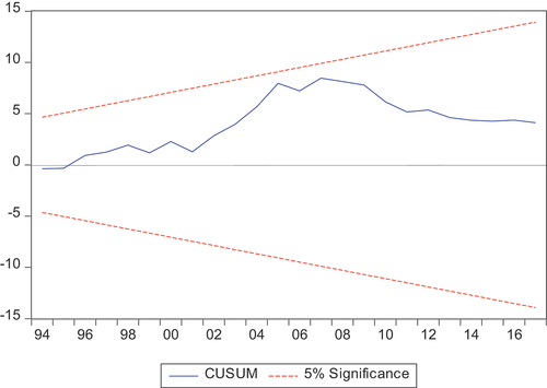
Figure 3. Cumulative sum of squared recursive residuals (CUSUMsq).

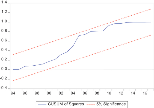
As shown in Figures 2 and 3, CUSUM and CUSUMsq plotted within the critical bounds at the 5 % level of significance, respectively. Thus, the parameters (coefficients) of the ARDL model for this study were stable.

5.8. Robustness analyses

The results of the ARDL model were validated in two ways. First, two alternative estimators (FMOLS and CCR) were used. Second, a different proxy for the main independent variable (fiscal capacity) was utilised. Results of the sensitivity analyses are presented and discussed in sections 5.8.1 and 5.8.2.

5.8.1. Sensitivity analysis using alternative estimators

For robustness of results, the FMOLS method by Phillips and Hansen (1990) and the CCR approach of Stock and Watson (1993) were applied. Just like the ARDL model, these estimators deal with the bias arising from endogeneity (Chen et al., 2017; Merlin & Chen, 2021; Rjoub et al., 2021; Tripathy & Mishra, 2021). In the present analysis, there was a need to account for the endogeneity (reverse causality) between PHE and GDP. Table 9 reports the results of the FMOLS and CCR methods.

Table 9. Regression results of FMOLS and CCR

Variable	FMOLS	CCR
lnREV	0.4911*** (0.0981)	0.4741*** (0.1094)
lnGDP	1.0990** (0.4338)	1.2415** (0.5087)
lnURB	−0.2062 (0.9039)	−0.3761 (0.9503)
lnDEBT	−0.0758 (0.2237)	−0.0404 (0.2060)
lnAGE	0.7913 (1.8991)	1.1153 (1.9657)
Constant	−11.4050 (5.6957)	−12.8336 (6.2098)**
R-squared Adjusted R^2 Observations	0.7951 0.7621 37	0.7938 0.7605 37

Standard errors are shown in parentheses.

Significance levels are shown by asterisks (***p < 0.01, **p < 0.05).

From the sensitivity analysis performed using the FMOLS and CCR, the results of the ARDL model are valid. The robustness checks show that both REV and GDP are significant determinants of PHE in Zimbabwe. Moreover, both the FMOLS and the CCR validate the earlier result from the ARDL model that PHE in the country is a luxury good—the income elasticity coefficient is greater than one. According to the results of the FMOLS, when GDP increases by 1%, PHE rises by 1.1%. Similarly, a 1% increase in fiscal capacity causes PHE to rise by 0.49%. The CCR results show that PHE rises by 1.24% following a 1% increase in GDP, while a 1% rise in fiscal capacity leads to a 0.47% increase in PHE.

5.8.2. Sensitivity analysis with an alternative proxy for fiscal capacity

Robustness analysis was also performed with fiscal capacity being measured as the ratio of general government final consumption expenditure to GDP, a proxy adopted by Behera and Dash (2020) and Sfakianakis et al. (2021). Three estimators, namely the ARDL model, the FMOLS approach, and the CCR method were applied. Results of the estimations are shown in Table 10.

Table 10. Regression results with GGCE as the proxy for fiscal capacity

Variable	ARDL	FMOLS	CCR
lnGGCE	0.2058 (0.1626)	0.5856*** (0.1201)	0.5772*** (0.1290)
lnGDP	2.0508*** (0.4580)	1.1974*** (0.4231)	1.2560** (0.4830)
lnURB	−1.8738 (0.9234)	−0.7694 (0.8902)	−0.8394 (0.9111)
lnDEBT	0.0511 (0.2859)	0.1158 (0.2341)	0.1318 (0.2066)
lnAGE	0.3201 (1.9462)	1.5632 (1.8946)	1.6711 (1.9381)
Constant	−10.1451*** (1.5800)	−12.7221** (5.6490)	−13.2705** (6.0376)
R-squared Adjusted R^2 Observations	0.8582 0.8346 36	0.7608 0.7223 37	0.7610 0.7224 37

Standard errors are shown in parentheses.

Significance levels are shown by asterisks (***p < 0.01, **p < 0.05).

From the results in Table 10, all the three estimators (ARDL, FMOLS, and CCR) have confirmed a positive and significant relationship between PHE and GDP when fiscal capacity is proxied by GGCE. Thus, whether fiscal capacity is measured as the ratio of tax revenue to GDP or the ratio of government final consumption expenditure to GDP, the variable remains a statistically significant positive determinant of PHE in Zimbabwe. Also, the conclusion that PHE in Zimbabwe is a luxury good has been maintained. Although the coefficient for GGCE is positive in the ARDL model, the variable is insignificant at the 5% level. Nonetheless, the same fiscal capacity variable is a significant positive determinant of PHE in the FMOLS and CCR estimations.

Besides using three estimators and an alternative proxy of fiscal capacity for the robustness analysis, it was also worthwhile to validate the results with a different measure of PHE. For example, rather than measuring the dependent variable as PHE (% of GDP), the per capita dollar amounts at current or constant prices, or in terms of purchasing power parity (PPP) could be utilised. However, time series data on Zimbabwe spanning the period 1980–2017 for such measures of PHE could not be obtained. Thus, the study relied on a single measure, PHE as a percentage of GDP.

6. Discussion

With regards to the main variable in the analysis, fiscal capacity, a positive and significant relationship with PHE was found, both in the long-run and in the short-run. This result is in line with previous studies in this area (Hooda, 2016; Behera & Dash, 2019, 2020; Murshed et al., 2020; Sfakianakis et al. 2021), and most importantly, supported by three separate studies that included Zimbabwe in panel regressions (Xu et al. 2011; Micah et al., 2019; Murshed et al., 2017). Hooda (2016) obtained a positive relationship between fiscal capacity and PHE in Indian states. Similar findings were obtained by Behera and Dash (2019) on a panel of 85 LMICs, Micah et al. (2019) in a study involving 46 Sub Saharan African countries, and Behera and Dash (2020) using data on nine countries in South-East Asia. Murshed et al. (2017) and Murshed et al. (2020) also confirmed a positive relationship between fiscal capacity and social spending in panels of 97 and 84 developing countries, respectively. The positive impact of fiscal capacity on PHE found in the current study means that during the period under consideration (1980–2017), the health sector has been one of the government’s priorities; budgetary allocations generally increased when more resources became available. Makochekanwa and Madziwa (2016) also support this observation and argue that, over the years, the Ministry of Health and Child Care (MoHCC) has remained one of the top five out of more than 15 ministries in terms of treasury allocations. Micah et al. (2019) found that Southern African governments, including Zimbabwe, have prioritized the health sector in terms of financing. The authors further argue that such high PHE is necessary, particularly given the fight against the HIV/ AIDS pandemic.

Equally important is for the government to fulfil the Abuja (2001) target of allocating at least 15% of the national budget to healthcare; during the years 2010–2021, on average, 10.65% was allocated to health (MoFED budget estimates 2015–2020; World Health Organisation (WHO), 2016). Moreover, the government needs to move towards achieving a minimum of 5% PHE to GDP ratio recommended for the attainment of UHC (WHO 2010; McIntyre et al., 2017). The data used in this study shows that from 1980 to 2017, government health expenditure (as a percentage of GDP) averaged 2.63%.

The study also established that GDP positively and significantly influence PHE in the long-run as well as the short-run. This means that growth in national income is good for PHE as this enhances the availability of fiscal resources. In a panel study of 84 developing countries, Murshed et al. (2020) found that GDP growth impacted positively on social protection expenditure. A related variable that has been extensively used in investigating the determinants of PHE is income, measured as per capita GDP. In the majority of the studies, a positive relationship between per capita GDP and PHE was found (Abbas & Hiemenz, 2013; Hooda, 2016; Murshed et al., 2017; Tajudeen et al. 2018; Micah et al., 2019; Sfakianakis et al. 2021). Thus, the results of the present study are in tandem with existing literature. The results also support Micah et al. (Micah et al., 2019: 9)’s conclusion that ” … improved economic conditions and strong economic growth are good things for the health sector”. Data from WB (2021) shows that although economic growth in Zimbabwe was positive for most of the years since 1980, the years 1999–2008 represented a crisis period in that the country lost a cumulative 64.63% in GDP. However, starting from 2009 annual real GDP growth rates of up to 19.7% in some years were witnessed, and as highlighted above, such conditions are conducive for the mobilization of healthcare resources.

7. Conclusion

Using time series data for the period 1980–2017, the study investigated the relationship between fiscal capacity and PHE in Zimbabwe. To analyse this relationship, an ARDL model was applied. Urbanisation, external debt, GDP, and the proportion of the elderly population were added as control variables. The study established that fiscal capacity and GDP positively influence PHE in Zimbabwe. The positive relationship between fiscal capacity and PHE means that as more resources become available, allocating more funds to health has been a priority of the government of Zimbabwe. Also, an increase in GDP means an expansion of a country’s tax base as this brings forth an improvement in the ability to pay taxes by firms and households. This, in turn, leads to a general improvement in fiscal capacity, thus enabling the government to channel more resources to health. The study recommends that the government continues to prioritise the health sector in the national budget. Also, given the positive impact of GDP on PHE, the study recommends the government to implement measures to promote macroeconomic stability and economic growth.

Disclosure statement

No potential conflict of interest was reported by the author(s).

Additional information

Funding

The authors have no funding to report.

Notes on contributors

Tamisai Chipunza

Tamisai Chipunza is an Economics lecturer at the Midlands State University, Zimbabwe. He teaches microeconomics and investment analysis modules. He recently earned a PhD in Economics with the University of South Africa. His research interests are in development economics, focusing on health economics.

Senia Nhamo

Senia Nhamo is a senior lecturer and Professor of Economics at the University of South Africa. She teaches econometrics, environmental economics and microeconomics. Her research interests are on the economic empowerment of women in fragile states, green growth indicators, and Agenda 2063 for Africa.

Notes

1. For the period 2005–2017, general government revenue to GDP data from IMF (2021) was used as a proxy for tax revenue to GDP ratio. The values were not significantly different from the tax to GDP ratios reported by WB (2021) (which were not utilised because of missing values for the years 2013 and 2014). It is worth noting that in Zimbabwe, non-tax revenue has generally constituted less than 10% of total government revenue (Government of Zimbabwe and WB 2017).

2. Prior knowledge of the order of integration of the variables is not necessary if the F-statistic of the bounds test lies outside the critical values (Pesaran, 2015; Pesaran et al., 2001).

3. The Akaike Information Criterion (AIC) and the Schwartz-Bayesian Information criteria (SBIC or SIC) are widely used in determining optimal lag lengths. The AIC gives the largest lag length possible whilst the SIC provides the smallest.

References

- Abbas, F., & Hiemenz, U. (2013). What determines public health expenditures in Pakistan? Role of income, urbanization and unemployment. Economic Change and Restructuring, 46(4), 341–20. https://doi.org/10.1007/s10644-012-9130-7
- Abuja Declaration on HIV/AIDS Tuberculosis and Other Related Infectious Diseases, (2001). https://au.int/sites/default/files/pages/32894-file-2001-abuja-declaration.pdf
- Afonso, A., Jalles, J. T., & Venâncio, A. (2021). Structural Tax Reforms and Public Spending Efficiency. Open Economies Review. https://doi.org/10.1007/s11079-021-09644-4
- Aladejare, S. A. (2019). Testing the Robustness of Public Spending Determinants on Public Spending Decisions in Nigeria. International Economic Journal, 33(1), 65–87. https://doi.org/10.1080/10168737.2019.1570302
- Awdeh, A., & Hamadi, H. (2019). Factors hindering economic development: Evidence from the MENA countries. International Journal of Emerging Markets, 14(2), 281–299. https://doi.org/10.1108/IJoEM-12-2017-0555
- Azolibe, C. B., Nwadibe, C. E., & Okeke, C. M. G. (2020). Socio-economic determinants of public expenditure in Africa: Assessing the influence of population age structure. International Journal of Social Economics, 47(11), 1403–1418. https://doi.org/10.1108/IJSE-04-2020-0202
- Baltagi, B. H. (2008). Econometric analysis of panel data. John Wiley & Sons.
- Baltagi, B. H., & Moscone, F. (2010). Health care expenditure and income in the OECD reconsidered: Evidence from panel data. Economic Modelling, 27(4), 804–811. https://doi.org/10.1016/j.econmod.2009.12.001
- Barkat, K., Sbia, R., & Maouchi, Y. (2019). Empirical evidence on the long and short-run determinants of health expenditure in the Arab world. Quarterly Review of Economics and Finance, 73, 78–87. https://doi.org/10.1016/j.qref.2018.11.009
- Baskaran, T., & Bigsten, A. (2013). ‘Fiscal Capacity and the Quality of Government in Sub-Saharan Africa’, World Development. Elsevier Ltd, 45, 92–107. https://doi.org/10.1016/j.worlddev.2012.09.018
- Behera, D. K., & Dash, U. (2018). ‘The impact of macroeconomic policies on the growth of public health expenditure: An empirical assessment from the Indian states’, Cogent Economics and Finance. Cogent, 6, 1. https://doi.org/10.1080/23322039.2018.1435443
- Behera, D. K., & Dash, U. (2019). Impact of macro-fiscal determinants on health financing: Empirical evidence from low-and middle-income countries. Global Health Research and Policy, 4(1), 1–13. https://doi.org/10.1186/s41256-019-0112-4
- Behera, D. K., & Dash, U. (2020). Healthcare financing in South-East Asia: Does fiscal capacity matter ? International Journal of Healthcare Management, 13(s1), s375–s384. https://doi.org/10.1080/20479700.2018.1548159
- Besley, T., & Persson, T. (2013). Handbook of Public Economics. Taxation and Development. https://doi.org/10.1016/B978-0-444-53759-1.00002-9
- Chaabouni, S., & Abednnadher, C. (2014). The determinants of health expenditures in Tunisia: An ARDL bounds testing approach. International Journal of Information Systems in the Service Sector, 6(4), 60–72. https://doi.org/10.4018/ijisss.2014100104
- Chandiwana, S. K., Moyo, I., Woelk, G., Sikosana, P., Braveman, P., & Hongoro, C. (1997). The Essential Step: An Interim Assessment of Equity in Health in Zimbabwe, A report prepared for the workshop on a Situational and Trend Analysis of Equity in Health and Health Care in Zimbabwe. Government Printers.
- Chen, G. S., Yao, Y., & Malizard, J. (2017). Does foreign direct investment crowd in or crowd out private domestic investment in China? The effect of entry mode. Economic Modelling, 409–419. https://doi.org/10.1016/j.econmod.2016.11.005
- Chowdhury, A. R., & Murshed, S. M. (2016). ‘Conflict and fiscal capacity’, Defence and Peace Economics. Routledge, 27(5), 583–608. https://doi.org/10.1080/10242694.2014.948700
- Common Market for Eastern and Southern Africa (COMESA)., (2020) COMESA health expenditure. https://comstat.comesa.int/ofnftuf/comesa-health-expenditure?country=Zimbabwe
- Dhliwayo, R. (2001). The Impact of Public Expenditure Management under ESAP on basic social services: Health and Education. Department of Economics, University of Zimbabwe. http://www.saprin.org/zimbabwe/research/zim_public_exp.pdf
- Dhoro, N. L., Chidoko, C., Sakuhuni, R. C., & Gwaindepi, C. (2011). Economic Determinants of Public Health Care Expenditure in Zimbabwe. International Journal of Economics Research, 13–25. www.ijeronline.com/documents/volumes/…/ijer20110206ND(2).pdf
- Friedman, M. (1978). The Limitations of Tax Limitation. Policy Review, 7–14.
- Gbaka, S., Iorember, P. T., Abachi, P. T., & Obute, C. O. (2021). Simulating the macroeconomic impact of expansion in total government expenditure on the economy of Nigeria. International Social Science Journal, 71(241–242), 283–300. https://doi.org/10.1111/issj.12289
- Getzen, T. E. (2000). Health care is an individual necessity and a national luxury: Applying multilevel decision models to the analysis of health care expenditures. Journal of Health Economics, 19(2), 259–270. https://doi.org/10.1016/S0167-6296(99)00032-6
- Government of Zimbabwe and World Bank, (2017) ‘Zimbabwe public expenditure review. 2017, volume 1: Cross cutting issues’. https://openknowledge.worldbank.org/handle/10986/27649
- Hanke, S. H., & Kwok, A. K. F. (2009). On the measurement of Zimbabwe’s hyperinflation. Cato Journal, 29(2), 353–363. https://s.libertaddigital.com/doc/estudio-de-la-hiperinflacion-en-zimbabue-18931689.pdf
- Hartwig, J. (2008). What drives health care expenditure?-Baumol’s model of “unbalanced growth” revisited. Journal of Health Economics, 27(3), 603–623. https://doi.org/10.1016/j.jhealeco.2007.05.006
- Hassoun, S. E., Adda, K. S., & Sebbane, A. H. (2021). ‘Examining the connection among national tourism expenditure and economic growth in Algeria’, Future Business Journal. Springer Berlin Heidelberg, 7(1), 1–9. https://doi.org/10.1186/s43093-021-00059-8
- Hooda, S. K. (2016). ‘Determinants of Public Expenditure on Health in India: A Panel Data Analysis at Sub-National Level’, Journal of Quantitative Economics. Springer India, 14(2), 257–282. https://doi.org/10.1007/s40953-016-0033-8
- Hsiao, C. (2007). Panel data analysis-advantages and challenges. Test, 16(1), 1–22. https://doi.org/10.1007/s11749-007-0046-x
- International Monetary Fund (IMF)., 2021. World Economic Outlook database, https://www.imf.org/en/Countries/ZWE
- Jaén-García, M. (2020). Tax-spend, spend-tax, or fiscal synchronization. A wavelet analysis. Applied Economics, 52(28), 3023–3034. https://doi.org/10.1080/00036846.2019.1705238
- Jakovljevic, M., Liu, Y., Cerda, A., Simonyan, M., Correia, T., Mariita, R. M., Kumara, A. S., Garcia, L., Krstic, K., Osabohien, R., Toan, T. K., Adhikari, C., Chuc, N. T. K., Khatri, R. B., Chattu, V. K., Wamg, L., Wijeratne, T., Kouassi, E., Khan, H. N., & Varjacic, M. (2021). The Global South political economy of health financing and spending landscape–history and presence. Journal of Medical Economics, 24(S1), 25–33. https://doi.org/10.1080/13696998.2021.2007691
- Jakovljevic, M., Ranabhat, C. L., Ibrahim, M. I. M., & Teixeira, J. (2021). Editorial: Universal Health Coverage: The Long Road Ahead for Low- and Middle-Income Regions. Frontiers in Public Health, 9(November), 1–3. https://doi.org/10.3389/fpubh.2021.746651
- Jibir, A., & Aluthge, C. (2019). ‘Modelling the determinants of government expenditure in Nigeria’, Cogent Economics and Finance. Cogent, 7, 1. https://doi.org/10.1080/23322039.2019.1620154
- Khan, M. A., & Husnain, M. I. U. (2019). ‘Is health care a luxury or necessity good? Evidence from Asian countries’, International Journal of Health Economics and Management. Springer US, 19(2), 213–233. https://doi.org/10.1007/s10754-018-9253-0
- Kumar, N. N., & Patel, A. (2022). Modelling the association between tourism and real exchange rates. Journal of Policy Research in Tourism, Leisure and Events, 1(1), 1–17. https://doi.org/10.1080/19407963.2022.2107656
- Linhares, F., Nojosa, G., & Bezerra, R. (2021). Changes in the revenue–expenditure nexus: Confronting evidence with fiscal policy in Brazil. Applied Economics, 53(44), 5051–5067. https://doi.org/10.1080/00036846.2021.1915463
- Lora, E., & Olivera, M. (2007). Public debt and social expenditure: Friends or foes? Emerging Markets Review, 8(4), 299–310. https://doi.org/10.1016/j.ememar.2006.12.004
- Madebwe, C., & Madebwe, V. (2017). Contextual background to the rapid increase in migration from Zimbabwe since 1990. Inkanyiso, 9(1), 27–36. https://www.ajol.info/index.php/ijhss/article/view/165505
- Mahi, M., Phoong, S. W., Ismail, I., & Isa, C. R. (2020). Energy-finance-growth nexus in ASEAN-5 countries: An ARDL bounds test approach. Sustainability (Switzerland), 12(1), 1–16. https://doi.org/10.3390/SU12010005
- Makochekanwa, A., & Madziwa, C. (2016). Impact of Public Health Expenditure on Health Status in Zimbabwe. University of Zimbabwe Business Review, 4(2), 64–76. https://ir.uz.ac.zw/bitstream/handle/10646/3868/Makochekanwa_Impact_of_public_health_expenditure_on_health_outcomes.pdf?sequence=1&isAllowed=y
- Manjokoto, C., & Ranga, D. (2017). Opportunities and challenges faced by women involved in informal cross-border trade in the city of Mutare during a prolonged economic crisis in Zimbabwe. Journal of the Indian Ocean Region, 25–39. https://doi.org/10.1080/19480881.2016.1270558
- Mansour, M. (2014). A tax revenue dataset for sub-Saharan Africa: 1980-2010. Revue d’Economie du Developpement, 22(3), 99–128. https://doi.org/10.3917/edd.283.0099
- McIntyre, D., Meheus, F., & Rottingen, J. A. (2017). What level of domestic government health expenditure should we aspire to for universal health coverage? Health Economics, Policy and Law, 12(2), 125–137. https://doi.org/10.1017/S1744133116000414
- Menegaki, A. N. (2019). The ARDL method in the energy-growth nexus field; best implementation strategies. Economies, 7(4), 1–16. https://doi.org/10.3390/economies7040105
- Merlin, M. L., & Chen, Y. (2021). ‘Analysis of the factors affecting electricity consumption in DR Congo using fully modified ordinary least square (FMOLS), dynamic ordinary least square (DOLS) and canonical cointegrating regression (CCR) estimation approach’, Energy. Elsevier Ltd, 232, 121025. https://doi.org/10.1016/j.energy.2021.121025
- Micah, A. E., Chen, C. S., Zlavog, B. S., Hashimi, G., Chapin, A., & Dieleman, J. L. (2019). Trends and drivers of government health spending in sub-Saharan Africa, 1995-2015. BMJ Global Health, 4(1), 1–10. https://doi.org/10.1136/bmjgh-2018-001159
- Ministry of Finance and Economic Development (MoFED)., (2015-2020). Budget estimates (various Issues).
- Ministry of Finance and Economic Development (MoFED)., (2019) ‘The 2020 national budget statement: Gearing for Higher Productivity, Growth and Job creation’. http://www.zimtreasury.gov.zw/index.php?option=com_phocadownload&view=category&id=54&Itemid=787
- Morris, S., Devlin, N., Parkin, B., & Spencer, A. (2012). Economic Analysis in Health Care. John Wiley & Sons.
- Munyuki, E., & Jasi, S. (2009) Capital flows in the health care sector in Zimbabwe: Trends and implications for the health system, EQUINET Discussion Paper Series 79. Rhodes University, Training and Research Support Centre, SEATINI, York University, EQUINET:. http://www.equinetafrica.org/bibl/docs/DIS79pppMUNYUKI.pdf
- Murshed, S. M., Badiuzzaman, M., & Pulok, M. H. (2017). Fiscal capacity and social protection expenditure in developing nations. The United Nations University.
- Murshed, S. M., Bergougui, B., Badiuzzaman, M., & Pulok, M. H. (2020). Fiscal Capacity, Democratic Institutions and Social Welfare Outcomes in Developing Countries. Defence and Peace Economics, 1–26. https://doi.org/10.1080/10242694.2020.1817259
- Murthy, V. N. R., & Okunade, A. A. (2016). ‘Determinants of U.S. health expenditure: Evidence from autoregressive distributed lag (ARDL) approach to cointegration’, Economic Modelling. Elsevier B.V, 59, 67–73. https://doi.org/10.1016/j.econmod.2016.07.001
- Nair, M., Samudram, M., & Vaithilingam, S. (2008). Malaysian money demand function revisited: The ARDL approach. Journal of Asia-Pacific Business, 9(2), 193–209. https://doi.org/10.1080/10599230801981944
- Narayan, P. K. (2005). The saving and investment nexus for China: Evidence from cointegration tests. Applied Economics, 37(17), 1979–1990. https://doi.org/10.1080/00036840500278103
- Newhouse, J. P. (1977). Medical care expenditure: A cross-national survey. The Journal of Human Resources, 12(1), 115–125. https://www.jstor.org/stable/145602
- Nyazema, N. Z. (2010). The Zimbabwe crisis and the provision of social services: Health and education. Journal of Developing Societies, 26(2), 233–261. https://journals.sagepub.com/doi/epdf/10.1177/0169796X1002600204
- Olayiwola, S. O., Bakare-Aremu, T. A., & Obiodun, S. O. (2021). Public health expenditure and economic growth in Nigeria: Testing of Wagner’s hypothesis. African Journal of Economic Review, 9(2), 130–150. https://www.ajol.info/index.php/ajer/article/view/205923
- Peacock, A. T., & Wiseman, J. (1961). Determinants of Government Expenditure. In A. T. Peacock & J. Wiseman (Eds.), The Growth of Public Expenditure in the United Kingdom. Princeton University Press. http://www.nber.org/chapters/c2304
- Pesaran, M. H. (2015). Time series and panel data econometrics. Oxford University Press.
- Pesaran, M. H., Shin, Y., & Smith, R. J. (2001). Bounds testing approaches to the analysis of level relationships. Journal of Applied Econometrics, 16(3), 289–326. https://doi.org/10.1002/jae.616
- Ricciuti, R., Savoia, A., & Sen, K. (2019). How do political institutions affect fiscal capacity? Explaining taxation in developing economies. Journal of Institutional Economics, 15(2), 351–380. https://doi.org/10.1017/S1744137418000097
- Rjoub, H., Odugbesan, J. A., Adebayo, T. S., & Wong, W. K. (2021). Sustainability of the moderating role of financial development in the determinants of environmental degradation: Evidence from Turkey. Sustainability (Switzerland), 13(4), 1–18. https://doi.org/10.3390/su13041844
- Rota, M. (2016). Military spending, fiscal capacity and the democracy puzzle. Explorations in Economic History, 60, 41–51. https://doi.org/10.1016/j.eeh.2015.11.002
- Sfakianakis, G., Grigorakis, N., Galyfianakis, G., & Katharaki, M. (2021). The impact of macro-fiscal factors and private health insurance financing on public health expenditure: Evidence from the OECD countries for the period 2000–2017. EuroMed Journal of Business, 16(1), 1–24. https://doi.org/10.1108/EMJB-03-2020-0029
- Shrestha, M. B., & Bhatta, G. R. (2018). Selecting appropriate methodological framework for time series data analysis. Journal of Finance and Data Science, 4(2), 71–89. https://doi.org/10.1016/j.jfds.2017.11.001
- Tajudeen, O. S., Tajudeen, I. A., & Dauda, R. O. (2018). Quantifying Impacts of Macroeconomic and Non-economic Factors on Public Health Expenditure: A Structural Time Series Model. African Development Review, 30(2), 200–218. https://doi.org/10.1111/1467-8268.12326
- Tripathy, N., & Mishra, S. (2021). The Dynamics of Cointegration Between Economic Growth and Financial Development in Emerging Asian Economy: Evidence from India. Vision. https://doi.org/10.1177/09722629211011811
- United Nations (UN). (2015). Transforming our World: The 2030 Agenda for Sustainable Development. https://sustainabledevelopment.un.org/content/documents/21252030%20Agenda%20for%20Sustainable%20Development%20web.pdf
- Van de Sijpe, N. (2012). Is foreign aid fungible? Evidence from the education and health sectors. The World Bank Economic Review, 27(2), 320–356. https://doi.org/10.1093/wber/lhs023
- Wagner, A. (1883). Finanzwissenschaft. Leipzig.
- World Bank (WB)., (2021) World Development Indicators. https://data.worldbank.org/indicator/SH.XPD.GHED.PC.CD?locations=ZW
- World Health Organisation (WHO)., 2016. Global Health Observatory data repository. https://apps.who.int/gho/data/node.main.GHEDGGHEDGDPSHA2011?lang=en
- Xu, K., Saksena, P., & Holly, A. (2011). ‘The Determinants of Health Expenditure : A Country-Level Panel Data Analysis’, Working Paper of the Results for Development Institute. http://www.who.int/health_financing/documents/report_en_11_deter-he.pdf.
- Yetim, B., Ilgun, G., Cilhoroz, Y., Demirci, S., & Konca, M. (2021). The socioeconomic determinants of health expenditure in OECD: An examination on panel data. International Journal of Healthcare Management, 14(4), 1265–1269. https://doi.org/10.1080/20479700.2020.1756112
- Zweifel, P., Felder, S., & Meiers, M. (1999). Ageing of population and health care expenditure: A red herring? Health Economics, 8(6), 485–496. https://doi.org/10.1002/(SICI)1099-1050(199909)8:6<485::