Climate variability impacts on agricultural output in East Africa

Abstract

This paper investigates whether the effects of weather variability in temperature and precipitation on agricultural output are short- or long-run. The contribution of this paper is twofold. First, the paper attempts to establish whether temperature or precipitation variability affects agricultural output in the short or the long run. Second, it examined whether the effects of temperature or precipitation variability on agricultural output are homogenous across East African countries. The results reveal that variability in temperature had a long-run impact on agricultural output, while variability in precipitation had a short-run effect. The findings also reveal that the long-run temperature variability effect was heterogeneous across East African countries, and to some extent, there is also evidence for the long-run effect of precipitation variability. These results are crucial in providing decision-makers and other interested parties a thorough evaluation of climate impacts and adaptation measures aimed at increasing agricultural production and food security.

Keywords:

• Climate variability
• agricultural output
• cross-sectional dependency
• heterogeneity

1. Introduction

Africa is one of the continents most susceptible to climate change and fluctuation (Niang et al., 2014). The continent also has a poor ability for adaptation, leaving it particularly exposed and vulnerable due to high rates of poverty, financial and technological limitations, as well as a significant reliance on agriculture supported by rain. This region has seen substantial seasonal variability in rainfall and a rise in mean, maximum, and minimum temperatures over the past few decades (Gan et al., 2016; S.H. Gebrechorkos et al., 2018). East Africa in particular is vulnerable to climate change and climate extremes since its countries are heavily dependent on rain-fed agriculture, have high levels of poverty, and have low levels of education (Kotikot et al., 2018; Okumu et al., 2021).

In fact, there are already visible direct effects of climate change on the economic growth of climate-dependent sectors like agriculture, which account for 43% of the East Africa’s gross domestic product (GDP) and affect the livelihoods of 80% of the region’s general population (Waithaka et al., 2013).

There has been an increase in the amount of research seeking to quantify the economic effects of climate change (Dell et al., 2009, 2012; Deschênes & Greenstone, 2007; Fisher et al., 2012; Kurukulasuriya & Mendelsohn, 2007; Lippert et al., 2009; Mendelsohn et al., 1994). For instance, the pioneering work of Mendelsohn et al. (1994) strengthened the theoretical underpinning of the Ricardian approach to the economic analysis of the impact of climate change on agriculture. Previously, the traditional production function technique had overlooked farmers’ ability to adapt to changing economic and environmental conditions.

In contrast, the Ricardian technique was a cross-sectional analysis that looked at how climate change and other variables influenced agricultural productivity over time (e.g., land values and farm revenues). This had the advantage of taking into account both the consequences of climate change and farmers’ ability to adapt to them. Mendelsohn et al. (1994) emphasised the need for adaptation efforts, in which farmers maintain their operations in accordance with climate volatility in order to reap higher benefits from agricultural output. Deschênes and Greenstone (2007) assessed the economic impact of climate change on US agricultural land by estimating the impact of random year-to-year temperature and precipitation fluctuations on agricultural profitability. According to their study, climate change would have increased annual revenues by US$1.3 billion or 4.0 percent, year. Large negative or positive effects are unlikely since the 95 percent confidence interval runs from $0.5 billion to $3.1 billion.

In addition, there is also growing concern about the impact of climate change variability on agricultural production per season, particularly in East Africa (Abraha-Kahsay & Hansen, 2016; Alboghdady & El-Hendawy, 2016; Kogo et al., 2021; Matiu, Ankerst, Menzel et al., 2017; Ochieng et al., 2016). For instance, Matiu, Ankerst, Menzel et al. (2017), climate variability explains over 60% of yield variability and is a significant factor influencing food output and farmers’ income. Abraha-Kahsay and Hansen (2016) found that precipitation variability has a negative effect on agricultural output in East Africa. Recently, Kogo et al. (2021) reveal that weather variability is also predicted to affect agricultural yields and patterns across a number of locations in Kenya.

However, these studies employed a variety of methods. Early empirical research on climate and agricultural output used cross-sectional regression analysis (Sachs & Warner, 1997), which is subject to omitted variable bias (Hsiang et al., (2017). As a result, cross-sectional regressions might lead to biased estimates of climate change and agricultural output. Early studies also examined the relationship between weather shocks and agricultural output use fixed effects panel regression models (Abraha-Kahsay & Hansen, 2016; Regan et al., 2019). Because fixed effects models account for unobserved time-invariant group heterogeneity, such as variations in institutions, these models are less susceptible to omitted variable bias. They have been used to investigate the link between weather variability and agricultural output (see, Abraha-Kahsay & Hansen, 2016; Barrios et al., 2008; Burke & Emerick, 2016; Deschênes & Greenstone, 2012; Fisher et al., 2012; Regan et al., 2019; Seo, 2013).

The inability of fixed effects models to account for long-term climatic variability is their limitation. The distinction between short-term extreme occurrences and long-term consequences is critical, since farmers may be better able to respond to long-term changes than to short-term or catastrophic events, by investing in either adaptation or mitigation. Mitigation and adaptation are two important tools for reducing the risks associated with climate variability.

Although there are few empirical research studies on long-run effects of climatic factors on agriculture output, they are crucial for policymakers to implement the policies that lessen the susceptibility of poor farmers to climate change. Examining the effects of climate change on agricultural production in this context, especially for certain African nations, under short-run and long-run distinctions, will add to the ongoing debate in the current literature on climate change and its effects on agriculture.

The studies of Blanc (2012), Kalkuhl and Wenz (2020), and Salahuddin et al. (2020) Ozdemir (2022) are among the exception, as they assess the long-run impact of climate change in the agriculture sector and the environment in general. Kalkuhl and Wenz (2020) explicitly assessed the effect of short-term weather shock and long-term climate change on the gross regional product and found that temperature affects productivity. If the global mean surface temperature rises by 3.5°C by 2100, worldwide production will be reduced by 7–14%, with much greater losses in tropical and poor nations. East Africa is particularly vulnerable to climate change and climate extremes due to its nations’ high levels of poverty, reliance on rain-fed agriculture, and low levels of education. This might undermine efforts put in place by East African governments.

According to the African Development Bank Group report 2019 (Attiaoui & Boufateh, 2019), East Africa economy is expected to grow at a healthy rate of 5.9 percent in 2019 and 6.1 percent in 2020. The nations with the fastest economic development are Djibouti, Ethiopia, Rwanda, Tanzania, and Kenya. However, the region still faces a number of downside risks that might jeopardize opportunities for development and economic progress. The major concerns include agriculture’s reliance on exporting primary commodities, susceptibility to natural disasters, and rising oil costs in nations that import oil.

Other study by Ozdemir (2022) looked at how the short- and long-term impacts of climate change on variables in agricultural productivity in Asia between 1980 and 2016 using dynamic and asymmetric panel autoregressive distributed lag estimators. He found that the climate change variable and agricultural productivity have a long-run relationship. Other studies like Gul et al. (2022) and Baig et al. (2022) also found that climate variables have a long-run effect on the agricultural products.

However, these studies did not account for the effect climate change variability on the agricultural output in the short and long run. Moreover, these studies did not account for the heterogeneous effect of climate variable of the agriculture across countries and mostly based outside Africa.

Our study joins the scant literature that assesses the long-term relationships. We investigate the relationship between climate variability (precipitation and temperature) and agricultural output across East African countries. Our study addresses two policy-relevant issues: (1) Does temperature or precipitation variability affect agricultural output, and if so, is the effect short- or long-term? (2) Is the effect of weather variability on agricultural output homogenous across East Africa?

The assumption that parameters are homogeneous across nations is one of the limitations of panel estimates. Based on the potential of different agricultural systems to expand, and the prevalence of such systems in each of the nations we studied, we expect the impact of temperature and precipitation to be heterogeneous.

Unlike recent studies, this study employs a set of second-generation panel data techniques that account for cross-sectional dependence and cross-country heterogeneity—issues that the first generation of panel data estimation techniques fail to address. To the best of our knowledge, Blanc (2012) and Ozdemir (2022) are the only studies that assess the impact of climate change on agricultural output in the long run by considering cross-country dependency. However, these studies assessed the effect of weather-related variables such as temperature and precipitation, but did not include the variability that exists in those variables.

Nowadays, the economies of the world have become more integrated, economically and financially, than they were a few decades ago; thus, not accounting for cross-sectional dependency (CD) across countries might lead to misleading results.

The results reveal that variability in temperature has a long-run impact on agricultural output, while variability in precipitation has a short-run effect. The results also show that the long-run temperature variability effect is heterogeneous across East African countries; to some extent, there was also evidence of the long-run effect of precipitation variability. After taking into consideration that countries are different in economic structure and dependent on each other, the findings reveal that precipitation variability effects are noticed in a few countries, such as Djibouti, Ethiopia, Rwanda and Uganda.

The structure of this paper is as follows: the literature is presented in section 2, and methodologies in section 3; section 4 reports findings, and section 5 concludes.

2. Literature review

Climate change can reduce food availability and affect the access to food and the quality of food. The reduced agricultural output may be the result of expected temperature rises, modifications to precipitation patterns, modifications to extreme weather events, and decreases in water availability. Therefore, the effects of climate change on agricultural production must thus be carefully considered by policymakers in the agriculture industry. Essentially, different settings may be used to study the impacts of climate change on agriculture, particularly the “Ricardian technique” and “time series/panel data approach” (Mendelsohn, 2008).

With the assumption that land rent would reflect the long-term net productivity of farmland based on survey or country-level data, the Ricardian approach focuses on the estimates of the cost of climate changes by analysing associations between land value and agro-climatic variables using the net revenue climate response function (Gbetibouo & Hassan, 2005; Kabubo-Mariara & Karanja, 2007; Lan-Huong et al., 2019; Mendelsohn & Dinar, 1999, 2003; Mendelsohn et al., 1994, 1996; Nguyen & Scrimgeour, 2022; De Salvo et al., 2013; Severen et al., 2018).

On the other hand, as more data have been available, time series/panel data models have gained popularity. Utilising this method, researchers have also looked at the relationship between the weather and the agricultural output (Sarker et al., 2012; Ortiz-Bobea et al., 2021; Mubenga-Tshitaka et al., 2021; Akpoti et al., 2022; Ozdemir, 2022; Song et al., 2022; Carr et al., 2022; Etwire et al., 2022). The effects of climate change on the physical and biological have been documented in the past (McCarthy et al., 2001; Parmesan & Yohe, 2003).

However, only a few studies have examined the short- and long-term effects of climate change on agricultural production using cutting-edge panel data approaches. For instance, Ozdemir (2022) looked at the short- and long-term impacts of climate change on agricultural productivity in Asia between 1980 and 2016 using dynamic and asymmetric panel autoregressive distributed lag estimators. The findings confirmed that there is existence of a long-run relationship between climate variables and only $\mathrm{C}{\mathrm{O}}_2$ emissions had an effect in the short run. Other studies investigated the effects of climate change factors in the long run. Gul et al. (2022) investigated how key food crop yields in Pakistan from 1985 to 2016 were affected by climate change factors like average temperature and rainfall patterns as well as non-climatic factors like the area devoted to crops with high yields, fertilizer use, and formal credit. After using an autoregressive distributed lag (ARDL), the results confirmed the long-run relationship between climatic and non-climatic factors to the major food crop yield in Pakistan. This study’s findings also pointed that temperature has a variety of effects on the yields of important food crops, whereas the production of key food crops is positively impacted by the area planted with these crops, the average rainfall, the fertilizer used, and formal credit. Baig et al. (2022) investigated the asymmetric dynamic relationship between climate change variables and the production of rice in India for the period spanning from 1991–2018. They considered the nonlinear autoregressive distributed lag (NARDL) model and Granger causality approach. The findings revealed that the mean temperature had a negative impact on the production of rice in the long run but positively affects the production in the short run. Other studies like Zaied & Cheikh (2015), Guntukula & Goyari (2020), Abbas (2020), Chandio et al. 2020a), Attiaoui & Boufateh (2019), Chandio et al. (2021), have investigated the long-run relationship between climate-related variables and the agricultural output and confirmed that the climate variables had a negative long-run effect on the agricultural output. In addition, Chandio et al. (2020b) provided evidence of short- and long-run effects of $\mathrm{C}{\mathrm{O}}_2$ emissions and average temperature on the cereal yield in Turkey, whereas average rainfall indicated a positive effect on the cereal yield in both short and long run. In contrast, Rehman et al. (2020) in their study investigating the climatic and carbon dioxide emissions impact on maize crop production in Pakistan found that there is a positive and long-run relationship between $\mathrm{C}{\mathrm{O}}_2$ emissions and maize crop production.

However, most of these study did not account for the cross-sectional dependence in the estimation. Assume that cross-sectional independence might lead to biased output and wrong conclusions (Lanzafame, 2014). Studies like Ozdemir (2022) are among the few that assess the long-run relationship between climate-related variables and agricultural output without assuming cross-sectional independence. Ozdemir (2022) showed that there is a long-run relationship between climate variables and agricultural productivity in Asian countries but only the $\mathrm{C}{\mathrm{O}}_2$ emissions had an impact in the short-run. They added that the $\mathrm{C}{\mathrm{O}}_2$ emissions effects turn from positive in the short-run to negative in the long-run.

Moreover, the importance of weather variability in the growing season has increased and has been noticed in the literature (Conway & Schipper, 2011; Mutai & Ward, 2000). In particular, the estimates of climate change in southern Africa have also revealed that variability and extreme events occurrences may become more common in the future (Tadross et al., 2005). In addition, concern over how much weather variability affects East African agriculture is growing (Wheeler at al., (2000); Barrios et al., 2008; Abraha-Kahsay & Hansen, 2016; Ochieng et al., 2016; Kogo et al., 2021). For instance, the false start of the growing season, which is a part of the beginning variability associated to agronomic drought and has a negative influence on agricultural productivity, is made worse by climate variability. Farmers frequently become confused about when to begin planting crops due to the false start of the growing season, which has an impact on seed germination and subsequent normal growth. Abraha-Kahsay and Hansen (2016) estimated a production functions for agricultural output in East Africa, using climatic variables broken down into growing and non-growing seasons. The results reveal that growing-season precipitation variability has a significant detrimental impact on plant growth after using the fixed-effect model.

Most of the conducted studies on the impact of climate change variability on the agriculture output consider precipitation and temperature as proxy of climate change. Additionally, they overlooked the possibility the presence of common factors that may contribute to the problem of cross-sectional dependency. African nations interact on a political, economic, social, and cultural level. They are also impacted by common phenomena like climate change, political unrest, the financial crisis, price shocks on global markets, energy use, etc. These articles do not consider cross-sectional dependency. They assume that countries are cross-sectional independent. When panel data is used, all of these variables may result in cross-sectional associations. Due to the assumption of cross-sectional independence, typical panel estimators produce biased outputs and draw the wrong conclusions (Lanzafame, 2014). Blanc (2012) and Ozdemir (2022) are the only studies conducted in Africa that have taken into account cross-sectional dependency in their analysis of the impact of weather-related variables on agricultural output, but they did not consider the impact of long-run weather variability. Our study too did not assume cross-sectional independence. Contrary to most studies on the impact of weather variability on agricultural output—such as Abraha-Kahsay and Hansen (2016); Kogo et al. (2021)

However, contrary to Blanc (2012) and Ozdemir (2022), who considered the long-run effects of temperature, rainfall and evaporation, did not consider the long-run effect of the variability of these weather variables. We also attempt to assess whether the effects of variability in temperature and precipitation on agricultural output are homogeneous in the long run.

3. Methodologies

Nowadays, it is essential to use the correct econometric approach when determining how changes in one or more factors may affect economic variables. Cross-sectional dependency (CD) and slope heterogeneity are two technical considerations that are overlooked by conventional econometric methods. Studies such as Bersvendsen and Ditzen (2021) and Espoir et al., (2022) propose adopting a proper econometric technique that considers two technical points: slope heterogeneity, and cross-sectional dependency.

First, because the world economies have become more financially and economically connected in the last three decades, testing for cross-sectional dependency (CD) before panel causality analysis is now required. The econometric literature has firmly determined that panel datasets are likely to show substantial CD as a result of this integration (Pesaran, 2004). This dependency may arise as a result of shared shocks, technical cross-country spillovers, market integration, and unobserved components that eventually become part of the error term (Espoir and Ngepah, 2021). If the errors (${\epsilon }_{i,t}$) are not independent across units, failing to account for cross-sectional dependency might lead to erroneous causality results (Herzer & Vollmer, 2012). Second, when it comes to slope heterogeneity, panel data methodologies estimate variations in between cross-sectional units by fixed constants (using fixed, random effects technique and the generalised method of moments). However, individual heterogeneity in slopes among cross-sectional units may be found in some panel datasets. Overlooking this variability may bias the results of causal relationships and lead to erroneous conclusions (Bersvendsen & Ditzen, 2021; Chang et al., (2015)). Ignoring slope heterogeneity incorrectly leads to biased findings (Pesaran & Smith, 1995).

For these reasons, this study examines the issue of cross-sectional dependence and slope heterogeneity before assessing the causal relationship between weather variability and agricultural output. Consider a Cobb-Douglass production function of agriculture; our study’s functional form is as follows:

(1) $Q=F\left(L,K,\mathrm{I}\right)$(1)

where $Q$ represents agricultural production, L stands for labour, K stands for capital such as land or machinery or animals, and I stands for additional elements such as fertiliser and irrigation. For this study, the baseline regression is presented in the following way:

$\begin{array}{rl}& In(outpu{t}_{it})={\beta }_0+{\beta }_{1}In(outpu{t}_{it-1})+{\beta }_{2}In(Labo{r}_{it})+{\beta }_{3}In(Lan{d}_{it})+{\beta }_{4}In(Machiner{y}_{it})\\ & +{\beta }_{5}In(Livestoc{k}_{it})+{\beta }_{6}In(Fertilize{r}_{it})+{\beta }_{7}In(Irrigatio{n}_{it})+{\beta }_{8}In(Temperature)\\ & +{\beta }_{9}In(Precipitation)+{\beta }_{10}Variabilit{y}^{Temperature}+{\beta }_{11}Variabilit{y}^{Precipitation}+{\mu }_i+{\epsilon }_{it}\end{array}(2)$

where $Outpu{t}_{it}$ and $Outpu{t}_{it-1}$ are the total agriculture production of the country and the lag of the total agriculture production I (i = 1,2,$\cdots n$) in year t(t = 1,2 $,\cdots ,T$). We include three capital inputs: Land, Machinery, and Livestock. We also include Labour, Fertiliser and Irrigation; ${\mu }_i$ is the unobserved time-invariant country-specific effect, and ${\epsilon }_{it}$ is the error term.

3.1. Econometric techniques

3.1.1. Cross-section dependence (CD)

When working with long-term panel data, it is possible to run into the cross-sectional dependency problem among cross-sectional units. An independent cross-sectional assumption would provide false findings. To counter this, Pesaran’s (2004) cross-sectional dependence test is used to determine if cross-sectional units are independent or dependent. The null hypothesis indicates independence, whereas the alternative hypothesis suggests a dependency,

(3) $C{D}_{statistics}=\sqrt{\frac{2t}{n\left(n-1\right)}\left({\sum }_{i=1}^{n-1}{\sum }_{j=i+1}^n\widehat{{\rho }_{i,j}}\right)}$(3)

in which the mean is zero and the variance is one, and $\rho$ denotes the pairwise correlation. For the null hypothesis, cross-sectional dependency does not exist; the alternative hypothesis implies that there is a cross-sectional dependency between cross-sectional units.

3.1.2. Unit root tests

To cope with cross-sectional dependence, it is important to use a consistent unit root econometric method. This study uses a second-generation unit root test. If there is no link between the cross-sections, according to the Pesaran CD test findings, first-generation unit root tests are utilised. If there is a dependence between cross-sections, however, second-generation unit root tests should be used. The second-generation tests that account for cross-sectional dependency are MADF (Taylor & Sarno, 1998), SURADF (Bai & Ng, 2004; Breuer et al., 2002), PANKPSS (Carrion-i-Silvestre et al., 2005), and CADF (Pesaran, 2007).

Pesaran (2007) introduced the CADF (Cross-Sectionally Augmented Dickey–Fuller Test) panel unit root test to account for cross-sectional dependency. This test, which may be used in both T > N and N > T situations, extends the basic ADF (Augmented Dickey–Fuller Test) regression with initial differences and lagged values of horizontal sections. The CIPS test examines the unit root characteristics of the whole panel; it is based on the CADF test. The estimation equation and hypotheses are as follows:

(4) $CIPS=N^{-1}{\sum }_{i=1}^{N}CAD{F}_t$(4)

Hypotheses of the CIPS test: $H_0$ indicates that the series is not stationary; $H_1$ indicates that the series is stationary. The cointegration technique used by Westerlund and Edgerton (2007) was selected for our investigation.

3.1.3. Panel LM bootstrap cointegration test

Westerlund and Edgerton (2007) developed a panel cointegration test that allows for dependency both within and between cross-sectional units, as well as correlation both within and between cross-sectional units, based on the Lagrange multiplier test of McCoskey and Kao (1998). In this test, a sieve sampling technique is used as a basis. It has the benefit of lowering the asymptotic test distortions substantially.

To conclude, all units in the panel are cointegrated according to the null hypothesis. In order to estimate long-term and short-term coefficients, the Pooled Mean Group Model (Panel ARDL) approach is employed.

3.1.4. Pooled Mean Group Model (Panel ARDL) and Dynamic Fixed Effect (DFE)

For panel cointegration analysis, M. H. Pesaran et al. (1999) proposed the PMG technique (Pooled Mean Group/Panel ARDL). A version of this approach has been developed for the ARDL model. This model allows estimating both short-term and long-term slope coefficients within the scope of the panel cointegration. According to this technique, constant variables, short-term coefficients and error terms can be changed across sections. While this technique does not allow for the change of long-term coefficients between units, it does allow for heterogeneity and the change of error-correction terms across groups in the short-term period. We can rename the explanatory variables in Equation (2) as $X$ for convenience; the Autoregressive distributive lag (ARDL) (p, q) dynamic specification can be written as

(5) $ln\left(Outpu{t}_{it}\right)={\sum }_{j=1}^p{\lambda }_{ij}ln\left(Outpu{t}_{i,t-j}\right)+{\sum }_{j=0}^q{\delta }_{ij}{X}_{i,t-j}+{\mu }_i+{\epsilon }_{it}$(5)

where Ln (Output) is the dependent variable and X is the k x 10 vector of the explanatory variables. ${\lambda }_{ij}$ denotes scalars, and ${\mu }_i$ represents the group-specific fixed effect, while p and q represent lags of dependent and independent variables changing from country to country. The fact that the variables here are cointegrated in the order of I (1). and the error terms I (0) indicates that there is a long-term relationship.

However, deviations from the long-term balance may occur. With a vector error correction model (VECM) to be established, deviations from long-term equilibrium can be expressed as:

(6) $\mathrm{\Delta }ln\left(Outpu{t}_{it}\right)={\varphi }_i\left(ln\left(Outpu{t}_{i,t-j}\right)-{\theta }_t^{\prime }{X}_{it}\right)+{\sum }_{j=1}^p{\lambda }_{ij}\mathrm{\Delta }ln\left(Outpu{t}_{i,t-j}\right)+{\sum }_{j=0}^q{\delta }_{ij}\mathrm{\Delta }{X}_{i,t-j}+{\mu }_i+{\epsilon }_{it}$(6)

(7) ${\varphi }_i=-\left(1-{\sum }_{j=1}^p{\lambda }_{ij}\right)$(7)

(8) ${\theta }_i=\frac{{\sum }_{j=0}^q{\delta }_{ij}}{\left(1-{\sum }_k{\lambda }_{ik}\right)}$(8)

(9) ${\lambda }_{ij}^{\ast }=-{\sum }_{m=j+1}^p{\lambda }_{im}\left(j=1,2,\dots ,p-1\right)$(9)

(10) ${\delta }_{ij}^{\ast }=-{\sum }_{m=j+1}^q{\delta }_{im}\left(j=1,2,\dots ,q-1\right)$(10)

where ${\varphi }_i$ stands for the speed of the error correction coefficient. If the error correction coefficient is zero, then there is no short-term connection, according to the definition. This coefficient is anticipated to be negative and smaller than 1. A large amount of time is required for this approach, because of the correlation between the error term and the estimators whose difference was subtracted from the average.

In our study, the time dimension is large, making this technique suitable. While the constant parameter may be changed in the Pooled Mean Group estimator, the slope parameter cannot be changed. The Dynamic Fixed Effect estimator, on the other hand, assumes that all parameters are constants. Pooled Mean Group Estimators and Dynamic Fixed Effect Estimators are used to estimate short- and long-term parameters in our investigation.

3.1.5. Random coefficient regression model

To check whether the slope coefficients are not consistent or homogeneous across panel units, the Swamy (1970) random linear regression model is used. The Swamy (1970) random-coefficients linear regression model does not need to impose the assumption of consistent parameters across panels.

Parameter heterogeneity is addressed as a stochastic variation in a random-coefficients model. Let assume that

(11) $Y_i=X_i{\beta }_i+{\in }_i$(11)

where $i=1,\dots ,m$ and ${\beta }_i$ is the coefficient vector (K x 1) for the cross-sectional unit, such that

${\beta }_i=\beta +v_i$, $E\left(v_i\right)=0$, $E\left(v_i,v_i^{\prime }\right)=\mathrm{\Sigma }$

To find $\hat{\beta }$ and $\widehat{\Sigma }$, the estimator is developed under the assumption that the cross-sectional specific coefficient vector ${\beta }_i$ is the result of a random process with a mean vector $\beta$ and covariance matrix $\mathrm{\Sigma }$,

(12) $Y_i=X_i{\beta }_i+{ }_i=X_i\left(\beta +v_i\right)+{ }_i=X_i\beta +\left(X_i{v}_i+{ }_i\right)=X_i\beta +{\omega }_i$(12)

where $E\left({\omega }_i\right)=0$, and

$E\left({\omega }_i{\omega }_i^{\prime }\right)=E\left\{\left(X_i{v}_i+{\in }_i\right){\left(X_i{v}_i+{\in }_i\right)}^{\prime }\right\}=E\left({\in }_i{\in }_i^{\prime }\right)+X_{i}E\left(v_i{v}_i^{\prime }\right)X_i^{\prime }={\sigma }_i^2\mathbf{I}+X_i\mathrm{\Sigma }{X}_i^{\prime }={\mathrm{\Pi }}_i$

where $\mathrm{\Pi }\equiv E\left(\omega \omega { }^{\mathrm{\prime }}\right)$ represents the block diagonal matrix with ${\mathrm{\Pi }}_i$, $i=1\text{ldotsm},$ along the main diagonal and zeroes elsewhere. The Generalised Least Squares (GLS) estimate of $\hat{\beta }$ is

(13) $\widehat{\beta }=\sum iXi{\Pi }_i^{-1}X-1\sum iXi{\Pi }_i^{-1}{y}_i={\displaystyle {\sum }_{i=1}^m{W}_i}{b}_i$(13)

where $W_i={\left\{{\sum }_{i=1}^m{\left(\mathrm{\Sigma }+v_i\right)}^{-1}\right\}}^{-1}{\left(\mathrm{\Sigma }+v_i\right)}^{-1}$

$b_i={\left(X_i^{\prime }{X}_i\right)}^{-1}{X}_i^{\prime }{y}_i$ and $V_i={\sigma }_i^2{\left(X_i^{\prime }{X}_i\right)}^{-1}$, representing the GLS estimator, is a matrix-weighted average of the panel-specific OLS estimators. The variance of $\hat{\beta }$ is:

(14) $Var\left(\hat{\beta }\right)={\sum }_{i=1}^m{\left(\mathrm{\Sigma }+V_i\right)}^{-1}$(14)

For more information about the slope and heterogeneity, see Swamy (1970).

In the presence of cross-sectional dependency and slope heterogeneity, using an econometric approach that imposes homogeneity requirements and ignores spatial interaction effects to assess panel causality between weather variability and agricultural output may provide incorrect results.

4. Data

We compiled a panel of nine nations (Burundi, Djibouti, Ethiopia, Kenya, Rwanda, Somalia, Sudan, Tanzania and Uganda) for our research, covering the period from 1961 to 2016. As in Abraha-Kahsay and Hansen (2016), the nine countries were chosen due to their similar crop production season characteristics. Data points were gathered from FAOSTAT (2011). As a dependent variable, the FAO’s net production index was considered for this study. It is considered a proxy for total production output and includes both crop and livestock production, as well as other agricultural outputs. Land input is considered a proxy for total area used for agricultural purposes, while machinery input is measured by the total number of tractors used. For livestock capital input, we employed the headcount for cattle, sheep and goats. Labour is measured by the percentage of the population working in agriculture. Agriculture’s fertiliser input is taken to be the number of metric tons of plant nutrients used. The consideration of these variables follows numerous studies (see, Abraha-Kahsay & Hansen, 2016; Barrios et al., 2008). Mean annual temperature and precipitation data were collected from the Climate Research Unit (CRU), as per Barrios et al. (2008) and Abraha-Kahsay and Hansen (2016).

We measured variability as the deviation of the previous year’s rainfall and temperature from the 30-year historical average during crop seasons (Amare et al., 2018). Variability is also referred to as rainfall and temperature anomalies. Figure 1 reports the general trends in precipitation and temperature during the period under consideration.

Figure 1. Trends in average precipitation and temperature in East Africa.

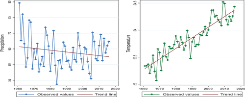
In general, the average annual temperature is increasing, and the trend becomes more significant as time goes by, while the opposite trend is observed for precipitation. The results are partly in line with studies such as S. H. Gebrechorkos et al. (2019), which reported that long-term seasonal rainfall did not show a significant trend (a decreasing trend in the east part of Ethiopia, an increasing trend in Kenya, and a decrease for Tanzania) during the long rainy season. The same study also reported that there is an increasing trend in the maximum and minimum temperatures for virtually the whole eastern region. Table A1 and A2 in the appendix report the descriptive statistics and the results of the Dumitrescu-Hurlin panel causality test for economic and climate variables.

5. Empirical analysis

To analyse the time-series characteristics, we took three preliminary steps. First, we looked for cross-sectional dependencies and slope heterogeneity between the variables across panel units. Second, we evaluated the panel unit root using specialised tests that accommodate the presence of cross-sectional dependency based on affirmative evidence. Finally, we examined whether there is a long-term or cointegration between the agricultural output and the rest of the covariates. If the unobserved dependency in the error terms is overlooked, it might lead to spurious results (Herzer & Vollmer, 2012).

For that, a cross-sectional dependency analysis was performed. The findings of the Pesaran CD test are shown in Table 1.

Table 1. Pesaran CD Test (cross-sectional dependency test)

Part A	CD-test	P-value	Variable	CD-test	P-value
Ln(Output)	29.37	0.00	Ln(Land)	29.70	0.00
Ln(Labour)	28.14	0.00	Ln(Machinery)	26.29	0.00
Ln(Livestock)	23.53	0.00	Ln(Irrigation)	10.60	0.00
Ln(Fertiliser)	6.16	0.00	Ln(Temperature)	30.22	0.00
Ln(Precipitation)	18.25	0.00
Part B: H. M. Pesaran et al. (2008) slope heterogeneity
					P-Value
Model (Equation 2)			$\tilde{\mathrm{\Delta }}$	17.05***	0.000
			${\tilde{\mathrm{\Delta }}}_{Adjusted}$	19.23***	0.000

Similar to the results in Table 1, the null hypothesis of no cross-sectional dependence is rejected at the 1% level of significance, and we can conclude that there is cross-sectional dependence in the data. As a result, these data demonstrate that the variables considered had considerable cross-sectional dependence throughout the period 1961–2016. This finding suggests that agriculture output and other covariates have substantial nearby interaction effects and likely to follow similar transmission mechanisms throughout East Africa. This is in line with one of the objectives of the East African Community (EAC) that strives to increase and strengthen cooperation among the partner nations and other regional economic communities for their mutual benefit in a variety of political, economic, and social spheres. Any study that assesses the impact of weather variability on agricultural output without taking cross-sectional dependence into account might result in misleading findings. Increased economic integration and trade volume and other natural phenomena processes like climate change might be linked to an increase in dependency, and the results of the cross-sectional analysis confirm this. These nine East African economies have an influence on each other’s economic development. Since there is cross-sectional dependency, the first-generation unit root tests are invalidated by these findings. Since cross-sectional units are dependent and heterogeneous, second-panel unit root tests will be used in this research. Pesaran (2007) CIPS unit root test results are considered in this study.

We also check for country-specific homogeneity in the slope coefficients. Using Equation (2), we use the H. M. Pesaran et al. (2008) slope heterogeneity test, and the outcomes are shown in Table 1, part B. At the 1% level of significance, the null hypothesis of slope homogeneity is tested and rejected for all panel units. This means that panel regressions that assume slope homogeneity constraints may provide false conclusions and misleading findings. Our study will account for the country-specific features by making use of appropriate estimation techniques.

The CIPS test, which is one of the second-generation unit root tests that considers cross-sectional dependence, is used in our study. The results are reported in Table 2. Based on the results, the order of integration is mixed, i.e. I (0) and I (1).

Table 2. Pesaran (2007) CIPS unit root test results

		A level		First difference
	Intercept	Intercept and trend	Intercept	Intercept and trend
Ln(Output)	−2.472	−2.605	−6.010***	−6.308***
Ln(Machine)	−2.718	−3.178	−5.005***	−5.331***
Ln(Land)	−1.667	−2.080	−5.645***	−5.734***
Ln(Livestock)	−2.326	−2.487	−6.019***	−6.203***
Ln(Labour)	−2.518	−1.049	−0.456***	−0.464***
Ln(Irrigation)	−2.252	−1.970	−5.721***	−5.912***
Ln(Fertiliser)	−3.526	−3.918	−6.190***	−6.420***
Ln(Temperature)	−5.194	−5.207	−6.250***	−6.420***
Ln(Precipitation)	−6.078	−6.309	−5.190***	−6.110***
Temperature variability	−5.103	−5.419	−6.150***	−6.395***
Precipitation Variability	−6.190	−6.420	−6.290***	−6.490***

Note: *** p < 0.01, ** p < 0.05, * p < 0.1, respectively. The critical values of CIPS test at 10%, 5% and 1% levels of significance are −2.21, −2.33 and −2.54 for Intercept, and −2.72, −2.83 and −3.04 for intercept plus trend, respectively.

Because some variables are stationary at level and others are stationary at the first difference, the predicted results reveal a mixed integration order. Using the Pesaran (2007) CIPS, the findings were achieved for both intercept and intercept and trend. Our results are consistent with those by Ozdemir (2022).

According to Table 2, Ln (machine), Ln (fertiliser), Ln (temperature), Ln (precipitation), Ln (temperature variability) and Ln (precipitation variability) are stationary at level. On the other hand, Ln (land) is not stationary. The findings of Ln (output), Ln (livestock), and Ln (irrigation) are complex. Ln (output) and Ln (livestock) are stationary at a 10% level of significance based on the intercept model, but non-stationary based on the intercept and trend model. This leads us to conclude that the two series are not stationary. After computing the first difference, the null hypothesis of panel non-stationary is rejected at a 1% level of significance for all variables. Due to this, we concluded that all our variables were integrated of order one (1). This means that there might be at least one long-term equilibrium relationship between the variables. Hence, there is a necessity for panel cointegration testing.

As cross-sectional units are Pedroni (1999, 2004) cointegration, metrics are incorrect; an appropriate econometric cointegration method should be considered for efficient results. Ignoring heterogeneous slope coefficients and cross-sectional dependencies in panel data might lead to biased and inconsistent conclusions (2020).

For these reasons, we employ the Westerlund and Edgerton (2007) cointegration test in order to confirm if the cointegration relationship exists in the long run. This is a panel cointegration test that uses error correction. Westerlund’s panel test for cointegration is more robust, according to Hossfeld (2010), because it deals with these issues by detecting structural breakdowns and cross-sectional dependency endogenously. In the presence of heterogeneous and dependent cross-sectional units, this method is appropriate. Using the Westerlund test, one may determine whether there is an error correction for each panel unit or for the complete panel. Statistical categories are broken down into two subcategories, each of which has two statistics in it. The two statistics of the first category are identified as the group mean statistics ($G_t,G_a$). The two statistics are known as the group mean statistics, while the second two statistics of the category are recognised as panel statistics ($P_t$, $P_a$). In both cases, they are pooling information concerning the error correction term along the cross-sectional dimension of the panel. The decision whether to reject the null hypothesis is based on the significance of the majority of the four statistics (Miti´c et al., 2017).

Table 3 reports the estimated Westerlund and Edgerton (2007) panel cointegration results.

Table 3. Westerlund And Edgerton (2007) Panel cointegration

	Intercept			Intercept and trend
Statistics	Values	Z-value	P-value	Values	Z-value	P-value
$G_t$	−2.0100	−0.7750	0.2190	−2.0380	−0.8700	0.1920
$G_a$	−11.7***	−2.5340	0.0060	−9.748*	−1.4360	0.0750
$P_t$	−5.678*	−1.3430	0.0900	−5.856*	−1.5220	0.0640
$P_a$	−10.8***	−4.4500	0.0000	−8.9***	−3.1960	0.0010

Note: p < 0.01***, < 0.05** and 0.1*, respectively

They reveal that under the null hypothesis of panel, no cointegration was ruled out. Except for $G_t$ (which is not significant), the remaining findings, for $G_a$, $P_t$, and $P_a$, respectively, are statistically significant at 1 and 10% levels of significance. It appears that the long-term cointegration relationship between variables is well supported by the calculated coefficients. This implies the existence of at least one long-run relationship between agricultural output and the regressors. Pooled Mean Group Analysis is employed to assess the short- and long-term relationships between the series in order to obtain coefficients.

Table 4 reports the outcomes of the pooled mean group (PMG) estimators.

Table 4. Pooled mean group (panel ARDL) model test results

Coefficients	Model (1)	Model (2)	Model (3)	Model (4)
Long-run coefficient
Ln(Machinery)	0.087 *** (0.000)	0.091*** (0.000)	0.073 *** (0.004)	0.101*** (0.001)
Ln(livestock)	0.5675*** (0.000)	0.565*** (0.000)	0.655*** (0.000)	0.567*** (0.000)
Ln(Labour)	0.349 *** (0.000)	0.338*** (0.000)	0.321 *** (0.000)	0.326*** (0.000)
Ln(Land)	0.648*** (0.000)	0.607*** (0.000)	0.607*** (0.000)	0.557 (0.000)
Ln(Fertiliser)	0.002 (0.858)	0.006 (0.564)	−0 .013 (0.134)	0.011 (0.356)
Ln(Temperature)	−5.781*** (0.000)	−5.969*** (0.000)	-	0.579* (0.085)
Ln(Precipitation)	-	0.165 (0.233)	-	−5.996 (0.000)
$Variabilit{y}^{Temp}$	−0.095** (0.043)	−0.090* (0.069)	-	-
$Variabilit{y}^{Precip}$	-	-	0.002 (0.311)	0.003 (0.520)
Short-run coefficient
$EC{T}_{\left(t-1\right)}$	−0.208*** (0.002)	−0.199*** (0.002)	−0.197*** (0.000)	−0.181*** (0.002)
$\mathrm{\Delta }Ln\left(Machinery\right)$	0.011 (0.864)	−0.001 (0.994)	0.017 (0.788)	0.004 (0.950)
$\mathrm{\Delta }Ln\left(Livestock\right)$	0.147** (0.046)	0.175** (0.017)	0.154** (0.020)	0.181** (0.011)
$\mathrm{\Delta }Ln\left(Labour\right)$	−1.088 (2.475)	−1.118 (2.492)	−1.064* (2.075)	−1.403 (2.310)
$\mathrm{\Delta }Ln\left(Land\right)$	0.302 (0.553)	0.469 (0.355)	0.389 (0.531)	0.395 (0.579)
$\mathrm{\Delta }Ln\left(Fertiliser\right)$	0.001 (0.916)	−0.001 0.898	−0.001 (0.930)	0.002 (0.888)
$\mathrm{\Delta }Ln\left(Irrigation\right)$	0.025 (0.548)	-	-	-
$\mathrm{\Delta }\mathrm{l}\mathrm{n}\left(Temperature\right)$	−0.223 (0.691)	−0.335 (0.515)	-	−0.200 (0.539)
$\mathrm{\Delta }Ln\left(Precipitation\right)$	-	0.049 (0.289)	-	0.171** (0.067)
$\mathrm{\Delta }Ln\left(aiabilit{y}^{Temp}\right)$	−0.002 (0.88)	−0.005 (0.673)	-	-
Observations	495	495	495	495

Standard errors in parentheses

*** p < 0.01, ** p < 0.05, * p < 0.1

Table 4 has two parts. The coefficients of the long-term relationship are presented in the first part. The short-term relationship coefficients are presented in the second part. We report a reduced version of the model, where the insignificant independent variables are eliminated successively. Models (1) and (2) consider only the impact of the temperature and variability in temperature on agricultural output, while Models (3) and (4) consider precipitation and variability in precipitation. Machinery, livestock, labour, and land have a positive and significant effect on agricultural output in the long run, based on the model (1) specification.

The estimated parameters for the physical inputs considered in this study do not vary across the models specified, and all have the expected signs. The specification in Model (4) confirms the findings except for the land coefficient, which is a positive but not significant coefficient. The irrigation coefficient showed no significance across all specifications and has been removed. The lack of significance of the irrigation parameter is not a surprise, as 95% of farming in this part of Africa is highly traditional, small-scale, and non-mechanised (Erikson et al., 2008). However, irrigation facilities are inadequate, since less than 4% of agricultural output in East Africa is generated by irrigation, compared to 33% in Asia (AfDB/IFAD, 2009).

We also find that machinery has a significant impact on agricultural output, contrary to the findings of Erikson et al. (2008) and Abraha-Kahsay and Hansen (2016). This is due to the fact that the fixed effect model used in those papers does not account for variable that varies over time. A specific country might through a national programme increase the number of machines used in the agriculture sector, while a pool mean estimator technique permits a greater degree of parameters heterogeneity in the long run than usual estimator techniques. In addition, it allows also heterogeneity in the short-run relationship (Simões, 2011).

East Africa, which is predominantly dominated by the agriculture sector, can adopt programme to promote this sector. For instance, Xia (2021) reveal that a small number of Chinese investors—many of whom have prior expertise in agricultural trade—have demonstrated increased interest in agricultural investment in countries like Kenya and Tanzania than other sectors. This has promoted the mechanization of the agricultural sector. This heterogeneity effect of machinery can be seen clearly in Table 6.

Table 6. Heterogeneous effect of climate variables on agricultural output

Variable	Burundi	Djibouti	Ethiopia	Kenya	Rwanda	Somalia	Sudan	Tanzania	Uganda
$Ln\left(Machinery\right)$	−0.00830	−0.01827	0.10539***	0.06084**	−0.01590	−0.02738	0.07765**	0.05661**	0.14745***
	(0.0240)	(0.02280)	(0.03431)	(0.02604)	(0.03083)	(0.02642)	(0.03517)	(0.02764)	(0.02877)
$Ln\left(Livestock\right)$	0.4114 ***	0.49559***	0.23904*	0.30267***	0.51345***	0.91774***	−0.06107	0.70162***	−0.11228
	(0.09125)	(0.05022)	(0.12870)	(0.08720)	(0.06358)	(0.07472)	(0.05831)	(0.18512)	(0.15489)
$Ln\left(Labour\right)$	0.08556	1.16237***	1.20105***	0.57441***	0.71111***	0.25175***	0.14081***	0.28452 **	−0.04051
	(0.09067)	(0.10866)	(0.07898)	(0.08869)	(0.06957)	(0.04413)	(0.04603)	(0.14328)	(0.14001)
$Ln\left(Land\right)$	−0.08389	0.11931	−0.72601***	−0.04133	0.83716***	−1.70396***	0.56085***	0.57568	2.34100***
	(0.20761)	(0.10253)	(0.18976)	(0.36763)	(0.23458)	(0.38194)	(0.14763)	(0.52084)	(0.59389)
$Ln\left(Fertiliser\right)$	0.04143	0.00393	0.09033***	0.07571***	0.02626	0.03488***	−0.05340	0.01965	0.20574***
	(0.02714)	(0.00818)	(0.03356)	(0.01138)	(0.01681)	(0.01164)	(0.03559)	(0.02065)	(0.01958)
$Ln\left(Precipitation\right)$	−0.27004	0.72475***	−0.03842	−0.05367	1.10233***	0.00410	0.29691	0.39651*	0.07363
	(0.20389)	(0.19013)	(0.09759)	(0.19777)	(0.23225)	(0.19960)	(0.19919)	(0.23725)	(0.28429)
$Ln\left(Temperature\right)$	0.14556	5.03644***	−0.23191	2.02294*	2.76571***	−2.13965**	−1.4054	4.02651***	4.11739***
	(0.40729)	(0.32586)	(0.66974)	(1.07896)	(0.45648)	(1.13533)	(0.80911)	(0.93092)	(1.10957)
$Ln{\left(Variability\right)}^{Precip}$	−0.00234	0.00704**	−0.00897*	−0.00164	0.00989***	0.00078	0.00931	0.00409	0.00707*
	(0.00261)	(0.00324)	(0.00521)	(0.00329)	(0.00324)	(0.00747)	(0.01110)	(0.00301)	(0.00383)
$Ln{\left(Variability\right)}^{Temp}$	−0.02516	0.11009***	−0.09786***	−0.02080	0.04952	0.01055	−0.00474	−0.08516***	0.04907
	(0.03691)	(0.03015)	(0.03286)	(0.03396)	(0.03946)	(0.02934)	(0.03513)	(0.03311)	(0.03954)
Observations	504	504	504	504	504	504	504	504	504
Number of ids	9	9	9	9	9	9	9	9	9

Standard errors in parentheses

*** p < 0.01, ** p < 0.05, * p < 0.1

Looking at the effect of variable climate on agricultural output, we find that on average, temperature and variability in temperature have a negative and significant effect on agricultural output in the long run. Our findings are partly in line with Baig et al. (2022) who found show that mean temperature has a short-term positive impact on the output but a long-term detrimental impact. In general, temperature and precipitation variations affect crop yields, as do growing $\mathrm{C}{\mathrm{O}}_2$ concentrations in the atmosphere (Wheeler & Von Braun, 2013). Temperature and water quantity are key variables for crop growth; thus, greater temperatures have a detrimental impact on soil quality and soil moisture. However, temperature increases are most likely to have a negative influence on agricultural yields (Ottman et al., 2012). The high temperature observed in the long run is detrimental, as it increases water stress. A reduction in fuel emissions to keep global warming at 1.5 °C is therefore urgently required (IPCC, 2018).

For policy intervention, this information is crucial, as it shows that the impact of the increased temperature in the agricultural sector in East Africa is more of a long-run phenomenon. Any policy measure intending to reduce the effect of water stress will improve agricultural output, since precipitation and its variability tend to have an effect only in the short run. In East Africa, without irrigation the region’s agriculture is subject to rainfall unpredictability and dry periods, even during the rainy season (Mupangwa et al., 2006), putting more stress on the agricultural sector. Policymakers should coordinate efforts to invest in irrigation quickly, in order to ensure food security.

Looking at the short-term relationship, the second part of Table 4 reveals that the error correction coefficient is negative, as theoretically expected. The error correction coefficient is found to be statistically significant with the expected sign, which supports the cointegration test results. The speed of adjustment tends to increase when one considers Models (1) and (2), where the temperature is considered. The estimated coefficients for physical inputs have the expected sign, but are not significant—except for the labour coefficient, which does have a negative sign but is still not significant. This is because most driving force in the agriculture sector in the short run is climate-related variables than economic variables. The coefficients of temperature are not significant, but have the expected sign. We found that annual precipitation has a positive and significant impact on output in East Africa, while precipitation variability has a negative and significant effect on agricultural output in the short run—in line with Abraha-Kahsay and Hansen (2016), who found that growing variability is having a serious negative effect on East African agricultural output and that the effect is more pronounced during the main growing season. This is because the East Africa region in particular is characterised by an increase in weather variability, especially in the main growing seasons, spring and autumn (Conway & Schipper, 2011; Schreck & Semazzi, 2004).

Table 5 reports findings from the dynamic fixed-effect model and consists of two parts.

Table 5. Dynamic fixed effect (DFE) model test results

Coefficients	Model (1)	Model (2)	Model (3)	Model (4)
Long-run coefficient
Ln(Machinery)	− 0.042 (0.067)	−0.049 (0.066)	−0.045 (0.065)	−0.047 (0.066)
Ln(livestock)	0.391*** (0.128)	0.423*** (0.127)	0.396*** (0.115)	0.428*** (0.128)
Ln(Labour)	0.259** (0.111)	0.255*** (0.109)	0.284*** (0.104)	0.280*** (0.104)
Ln(Land)	0.391 (0.352)	0.393 (0.345)	0.408 (0.320)	0.445 (0.344)
Ln(Fertiliser)	−0.013 (0.042)	−0.008 (0.041)	−0.006 (0.042)	−0.003 (0.041)
Ln(Temperature)	−1.286 (4.124)	−0.830 (0.346)	-	0.688 (0.526)
Ln(Precipitation)	-	0.473 (4.054)	-	0.676 (3.594)
$Ln(Variabilit{y}^{Temp})$	−0.115 (0.177)	−0.131 (0.175)	-	-
$Ln\left(Variabilit{y}^{Precip}\right)$	-	-	0.005 (0.008)	0.006 (0.012)
Short-run coefficient
$EC{T}_{\left(t-1\right)}$	−0.109*** (0.020)	−0.111*** (0.019)	−0.109*** (0.0192)	−0.109 (0.0193)
$\mathrm{\Delta }Ln\left(Machinery\right)$	−0.008 (0.022)	−0.005 (0.022)	−0.006 (0.022)	−0.007 (0.021)
$\mathrm{\Delta }Ln\left(Livestock\right)$	0.079* (0.043)	0.077* (0.043)	0.081** (0.044)	0.078 (0.042)
$\mathrm{\Delta }Ln\left(Labour\right)$	−0.010 (0.052)	−0.017 (0.057)	−0.011 (0.054)	−0.019 (0.0549)
$\mathrm{\Delta }Ln\left(Land\right)$	0.377*** (0.136)	0.365*** (0.136)	0.371*** (0.135)	0.370*** (0.136)
$\mathrm{\Delta }Ln\left(Fertiliser\right)$	0.0008 (0.006)	−0.0002 (0.006)	−0.0003 (0.007)	−0.0002 (0.006)
$\mathrm{\Delta }\mathrm{l}\mathrm{n}\left(Temperature\right)$	0.168 (0.428)	0.167 (0.027)	-	0.223 (0.388)
$\mathrm{\Delta }Ln\left(Precipitation\right)$	-	0.044 (0.429)	-	0.071* (0.040)
$\mathrm{\Delta }Ln\left(Variabilit{y}^{Temp}\right)$	−0.006 (0.014)	−0.008 (0.015)	-	-
$\mathrm{\Delta }Ln\left(Variabilit{y}^{Precip}\right)$	-	-	0.0003 (0.001)	−0.0007 (0.0008)
Constant	1.099 (0.369)	−0.799 (0.518)	−0.696* (0.378)	−0.259 (1.089)
Observations	495	495	495	495

Standard errors in parentheses

*** p < 0.01, ** p < 0.05, * p < 0.1

The first part shows the coefficients of the long-run relationship, and the second reports the short-run relationship. Labour and livestock are significant, with the expected sign, in the long run. Other variables have the expected sign, except for machinery and fertiliser; but not all are significant.

Looking at climate variables, the results reveal that both temperature and precipitation are not significant, but have the expected sign. The variability in both temperature and precipitation is not significant in the long term.

The second part of Table 5 reports the short-run relationship. The error correctional model has the expected sign, and variables are significant across all specifications. Land and livestock are the only parameters that are significant with the expected sign across all specifications in the short run. Climate variables have the sign expected, but are not statistically significant.

Given that the PMG gives only the cross-heterogeneous effect in the short term and the weighted-average effect in the long term, it is also possible to obtain the heterogeneous long-run marginal effect of climate variability on output. According to PMG results, for instance, weather-related variables affect the agricultural output across nine countries in the same manner. These results contradict the IPCC (2007) that emphasises that even though climate change is a global phenomenon, its effects vary from one region to another depending on various socio-economic factors. It is crucial to assess the marginal effect of weather-related variables on each country under investigation.

We carry out the analysis one step further to investigate the heterogeneous effect of climate variables on agricultural output across the nine East African countries. Table 1, part B reports the results of H. M. Pesaran et al. (2008) and confirm that the slopes are heterogeneous. We apply the Swamy (1970) random coefficient linear regression model, which does not impose the assumption of constant parameters across the panel. The results are reported in Table 6.

The estimated coefficients for the physical outputs and climate variables do vary across countries. In Burundi, most of the inputs have the expected sign, but are not significant, except livestock input, which is significant, but without the long-run effect of climate variables on output. In Djibouti, labour and livestock are significant, with the expected sign, while other physical inputs have the expected signs, but are not significant, except that machinery does have a negative sign but is not significant. We found evidence of the impact of climate variables in this country. The average temperature and precipitation and their variability have an impact on agricultural output in the long run. In Ethiopia, machinery, labour, land and fertiliser are significant and positive, but the land coefficient is negative and significant. Land in Ethiopia has deteriorated due to climate change, which has had a negative effect on agricultural output. Teshome (2016), for instance, reveals that an increase in temperature, a decrease in rainfall and abnormal precipitation are increasingly making households vulnerable in rural Ethiopia. This is in line with our findings: we found that annual temperature and precipitation have a negative long-term impact on agricultural output. This is in contrast to what we reported in Table 4, where the effect was only coming from temperature in the long run.

In Kenya, only the average temperature has a long-run impact on output. Machinery, livestock, labour and fertiliser have an impact on output in the long run in Kenya. Rwanda also shows a significant positive impact of the physical input parameters on the agricultural output; except for machinery, which is positive but not significant. Results show that in the long run, temperature and precipitation have an effect, but so does temperature variability. In Somalia, the land variability had a negative effect on agricultural output, confirming the presence of climate change in this region. Labour and fertiliser parameters are positive and significant. We find that only temperature has a negative impact in Somalia. In Tanzania and Uganda, temperature has a long-term impact on the agricultural sector, while no effect is observed in Sudan. In Tanzania, there is also the long-run impact of precipitation variability on output.

6. Conclusion

This empirical study aimed to investigate the relationship between weather variability and agricultural output in the long run. In particular, we investigated the relationship between precipitation and temperature and agricultural output across East African countries. The contribution of this paper is twofold. First, the paper attempted to establish whether temperature or precipitation variability affects agricultural output in the short or the long run. Second, it examined whether the effects of temperature or precipitation variability on agricultural output are homogenous across East African countries. For that, we considered economic data from the FAOSTAT from 1961 to 2016 and climate data from the Climate Research Unit (CRU). We first tested whether there was cross-sectional dependency in the data; if this had been the case, the first-generation panel econometric techniques would not have been applicable. Variability in temperature and precipitation are measured as the deviation of the previous year’s precipitation and temperature from the 30-year historical average. Variability is referred to as rainfall and temperature anomalies observed during the period under consideration. We found that variability in temperature had a long-run impact on agricultural output, while variability in precipitation had a short-run effect. We also found that the long-run temperature variability effect was heterogeneous across East African countries, and to some extent, there was also evidence for the long-run effect of precipitation variability.

As per our study findings, it is recommended that studies on the impact of climate change on agricultural output should consider the cross-sectional dependency that exists between countries, as countries do not have the same agricultural system. In addition, the effects of temperature and precipitation variability are different between the short run and the long run. The effect of temperature and precipitation variability on agricultural output is a specific-country reality, due to the different responses that have been put in place. Policies intended to promote irrigation in East Africa can have a significant impact; especially in the short run, precipitation variability is more serious in the short run. There should also be investment in technology, as agricultural technology provides farmers with several benefits including improved production, and crops that are more adaptable to climate change.

In addition, in order to increase crop production and achieve food security while reducing the challenges brought on by climate change, governments can play a critical role by encouraging appropriate farm-level adaptation measures, providing timely early warning information on seasonal climate forecasts, and developing supportive policies and investments.

Finally, there are several caveats to this study. First, results from this study are different from those of previous studies, as we attempted to investigate the long-run impact of weather variability on agricultural output. The generality of previous studies should be viewed with caution, as there is evidence of a substantial increase in weather variability in the growing seasons (Abraha-Kahsay & Hansen, 2016; Kogo et al., 2021; Ochieng et al., 2016). Future studies should investigate the long-run impact of growing season temperature and precipitation variability on agricultural output under the assumption of cross-dependency in the panel data.

In addition Kogo et al. (2021), revealed that climate change and variability would continue to have detrimental effect the crop production and food security to the already vulnerable communities in countries like Kenya. Future research should also consider investigating the long-run relationship between temperature and precipitation variability on different types of crops, as such effects cannot be captured when one uses an aggregate variable. This relationship might also be investigated at two levels: at the agricultural system and household level.

Disclosure statement

No potential conflict of interest was reported by the author(s).

Additional information

Funding

The authors received no direct funding for this research.

Appendix

Table A1. Descriptive statistics of economic and climate data

Variables	Mean	St. Dev.
Dependent variable
Output (in millions of international US dollars)	7444.88	5910.00
Independent variables
Physical
Land (1000 persons)	31,226.30	34,763.56
Labour (1000 of hectares)	19,964.49	26,190.84
Machinery	3057.55	3835.89
Livestock (Head count of cattle, sheep and goats, in millions)	28.20	31.30
Irrigation (1000 of hectares)	0.48	0.50
Fertiliser (1000 of hectares)	21,539.26	36,567.19
Climate variables
Temperature	23.83	2.97
Precipitation	64.11	34.65
$Variabilit{y}^{Temp}$	0.06	0.35
$Variabilit{y}^{Precip}$	−0.53	7.30
countries	9
Sample	504

Table A2. Results of the Dumitrescu–Hurlin panel causality test

	O	M	La	Li	Lo	Irr	Fe	T	P	VT	VP
O	–	1.77*	1.95**	2.92***	4.52***	0.83	0.40	0.11	−0.26	0.96	−0.64
		(0.08)	(0.05)	(0.003)	(0.000)	(0.408)	(0.67)	(0.91)	(0.79)	(0.34)	(0.52)
M	5.3***	–	6.6***	4.83***	8.74***	10.***	1.25	0.97	1.32	0.62	0.209
	(0.000)		(0.000)	(0.000)	(0.000)	(0.000)	(0.210)	(0.330)	(0.188)	(0.539)	(0.834)
La	1.52	1.83 *	–	4.02***	6.12***	3.8***	0.12	2.7***	2.40**	−0.13	2.30**
	(0.128)	(0.066)		(0.000)	(0.000)	(0.000)	(0.907)	(0.006)	(0.016)	(0.893)	(0.021)
Li	2.6***	0.43	6.3***	–	3.40***	1.70*	−0.04	3.3***	−0.01	0.82	−0.03
	(0.010)	(0.668)	(0.000)		(0.001)	(0.08)	(0.971)	(0.001)	(0.993)	(0.414)	(0.976)
Lo	23.***	12.7***	10.***	17.35***	–	4.2***	17.***	1.77*	2.93**	0.75	1.42
	(0.000)	(0.000)	(0.000)	(0.000)		(0.000)	(0.000)	(0.076)	(0.003)	(0.455)	(0.155)
Irr	2.85** (0.004)	12.1*** (0.000)	6.9*** (0.000)	1.46 (0.144)	2.69*** (0.007)	–	3.9*** (0.000)	2.36** (0.018)	0.44 (0.663)	−0.92 (0.356)	−0.32 (0.747)
Fe	4.2*** (0.000)	3.01*** (0.003)	0.149 (0.881)	1.92* (0.055)	1.01 (0.311)	0.016 (0.986)	–	0.30 (0.762)	0.68 (0.496)	−0.12 (0.914)	0.24 (0.809)
T	17.*** (0.000)	9.69*** (0.000)	15.*** (0.000)	8.7*** (0.000)	32.4*** (0.000)	14.*** (0.000)	3.6*** (0.000)	–	1.485 (0.137)	24.*** (0.000)	1.262 (0.206)
P	0.734 (0.462)	2.1** (0.034)	1.158 (0.246)	1.063 (0.287)	0.959 (0.337)	0.206 (0.836)	3.9*** (0.000)	0.078 (0.937)	–	−0.827 (0.407)	1.85* (0.064)
VT	5.4*** (0.000)	5.2*** (0.000)	5.4*** (0.000)	4.1*** (0.000)	4.8*** (0.000)	4.9*** (0.000)	1.183 (0.237)	6.8*** (0.000)	−0.749 (0.453)	–	−1.252 (0.210)
VP	0.002* (0.076)	2.5** (0.012)	0.11** (0.028)	−0.90* (0.067)	−0.523 (0.600)	−0.34** (0.030)	2.55** (0.011)	−0.794 (0.427)	−1.403 (0.161)	−1.121 (0.262)	–

Note: P-values are shown in parentheses, ***, **, * represents 1%, 5%, 10% level of significance respectively. O represents output, M (machine), La (land), Li (livestock), Lo (labour),Irr (Irrigation), Fe (fertilizer), T (temperature), P (precipitation), VT (variability in temperature), VP (variability in precipitation)

References

- Abbas, S. (2020). Climate change and cotton production: An empirical investigation of Pakistan. Environmental Science and Pollution Research, 27(23), 29580–25. https://doi.org/10.1007/s11356-020-09222-0
- Abraha-Kahsay, G., & Hansen, L. G. (2016). The effect of climate change and adaptation policy on agricultural production in Eastern Africa. Ecological Economics, 121, 54–64. https://doi.org/10.1016/j.ecolecon.2015.11.016
- AfDB/IFAD. (2009). AFDB/IFAD Joint Evaluation of their agricultural operations and policies in Africa, Rome: Draft Report. African Development Bank.
- Akpoti, K., Groen, T., Dossou-Yovo, E., Kabo-bah, A. T., & Zwart, S. J. (2022). Climate change-induced reduction in agricultural land suitability of West-Africa’s inland valley Landscapes. Agricultural Systems, 200, 103429. https://doi.org/10.1016/j.agsy.2022.103429
- Alboghdady, M., & El-Hendawy, S. E. (2016). Economic impacts of climate change and variability on agricultural production in the Middle East and North Africa region. International Journal of Climate Change Strategies and Management, 8(3), 463–472. https://doi.org/10.1108/IJCCSM-07-2015-0100
- Amare, M., Jensen, N. D., Shiferaw, B., & Cissé, J. D. (2018). Rainfall shocks and agricultural productivity: Implication for rural household consumption. Agricultural Systems, 166, 79–89. https://doi.org/10.1016/j.agsy.2018.07.014
- Attiaoui, I., & Boufateh, T. (2019). Impacts of climate change on cereal farming in Tunisia: A panel ARDL-PMG approach. Environmental Science Pollution Research, 26(13), 13334–13345. https://doi.org/10.1007/s11356-019-04867-y
- Baig, I. A., Chandio, A. A., Ozturk, I., Kumar, P., Khan, Z. A., & Salam, M. A. (2022). Assessing the long‑ and short‑run asymmetrical effects of climate change on rice production. Empirical Evidence from India, Environmental Science and Pollution Research, 29(23), 34209–34230. https://doi.org/10.1007/s11356-021-18014-z
- Bai, J., & Ng, S. (2004). A panic attack on Unit Roots and Cointegration. Econometrica, 72(4), 1127–1177. https://doi.org/10.1111/j.1468-0262.2004.00528.x
- Barrios, S., Ouattara, B., & Strobl, E. (2008). The impact of climatic change on agricultural production: Is it different for Africa. Food Policy, 33(4), 287–298. https://doi.org/10.1016/j.foodpol.2008.01.003
- Bersvendsen, T., & Ditzen, J. (2021). Testing for slope heterogeneity in Stata. The Stata Journal, 21(1), 51–80. https://doi.org/10.1177/1536867X211000004
- Blanc, E. (2012). The impact of climate change on crop yields in sub-Saharan Africa. American Journal of Climate Change, 1(1), 1–13. https://doi.org/10.4236/ajcc.2012.11001
- Breuer, B. B., McNown, R., & Wallac, M. (2002). Series-specific unit root tests with panel data. Oxford Bulletin of Economics and Statistics, 64(5), 527–546. https://doi.org/10.1111/1468-0084.00276
- Burke, M., & Emerick, K. (2016). Adaptation to climate change: Evidence from US agriculture. American Economic Journal: Economic Policy, 8(3), 104–140. https://doi.org/10.1257/pol.20130025
- Carrion-i-Silvestre, J. L., Barrio-Castro, T. D., & López-Bazo, E. (2005). Breaking the panels: An application to the GDP per capita. The Econometrics Journal, 8(2), 159–175. https://doi.org/10.1111/j.1368-423X.2005.00158.x
- Carr, T. W., Mkuhlani, S., Segnon, A. C., Ali, Z., Zougmoré, R., Dangour, A. D., Green, R., & Scheelbeek, P. (2022). Climate change impacts and adaptation strategies for crops in West Africa: A systematic review. Environmental Research Letters, 17(5), 053001. https://doi.org/10.1088/1748-9326/ac61c8
- Chandio, A. A., Jiang, Y., Rehman, A., & Rauf, A. (2020a). Short and long-run impacts of climate change on agriculture: an empirical evidence from China. International Journal of Climate Change Strategies Management,12(2), 201–221.
- Chandio, A. A., Jiang, Y., Akram, W., Adeel, S., Irfan, M., & Jan, I. (2021). Addressing the effect of climate change in the framework of financial and technological development on cereal production in Pakistan. Journal of Cleaner Production, 288, 125637. https://doi.org/10.1016/j.jclepro.2020.125637
- Chandio, A. A., Ozturk, I., Akram, W., Ahmad, W., & Mirani, A. A. (2020b). Empirical analysis of climate change factors affecting cereal yield: Evidence from Turkey. Environmental Science and Pollution Research, 27(11), 11944–11957. https://doi.org/10.1007/s11356-020-07739-y
- Chang, T., Gupta, R., Inglesi-Lotz, R., Simo-Kengne, B., Simithers, D., & Trembling, A. (2015). Renewable energy and growth: Evidence from heterogeneous panel of G7 countries using Granger causality. Renewable and Sustainable Energy Reviews, 52, 1405–1412. https://doi.org/10.1016/j.rser.2015.08.022
- Conway, D., & Schipper, E. L. F. (2011). Adaptation to climate change in Africa: Challenges and opportunities identified from Ethiopia. Global Environmental Change, 21(1), 227–237. https://doi.org/10.1016/j.gloenvcha.2010.07.013
- Dell, M., Jones, B. F., & Olken, B. A. (2009). Temperature and income: Reconciling new cross-sectional and panel estimates. American Economic Review, 99(2), 198–204. https://doi.org/10.1257/aer.99.2.198
- Dell, M., Jones, B. F., & Olken, B. A. (2012). Temperature shocks and economic growth: Evidence from the last half century. American Economic Journal Macroeconomics, 4(3), 66–95. https://doi.org/10.1257/mac.4.3.66
- De Salvo, M., Raffaelli, R., & Moser, R. (2013). The impact of climate change on permanent crops in an Alpine region. a Ricardian Analysis, Agricultural Systems, 118, 23–32. https://doi.org/10.1016/j.agsy.2013.02.005
- Deschênes, O., & Greenstone, M. (2007). The economic impacts of climate change: Evidence from agricultural output and random fluctuations in weather. American Economic Review, 97(1), 354–385. https://doi.org/10.1257/aer.97.1.354
- Deschênes, O., & Greenstone, M. (2012). The economic impacts of climate change: Evidence from agricultural output and random fluctuations in weather: Reply. American Economic Review, 102(7), 3761–3773. https://doi.org/10.1257/aer.102.7.3761
- Erikson, S., O’Brien, K., & Rosentrater, L. (2008). Climate Change in Eastern and Southern Africa: Impacts, Vulnerability and Adaptation. Global Environment Change and Human Security.
- Espoir, D. K. & Ngepah, N. (2021). Income distribution and total factor productivity: across-country panel. International Economics and Economic, 18, 661–698.
- Espoir, D. K. Mudiangombe, B. M., Bannor, F., Sunge, R., Mubenga-Tshitaka, J. L. (2022). CO2 emissions and economic growth: Assessing the heterogeneous effects across climate regimes in Africa. Science of the Total Environment, 804, 150089. https://doi.org/10.1016/j.scitotenv.2021.150089
- Etwire, P. M., Koomson, I., & Martey, E. (2022). Impact of climate change adaptation on farm productivity and household welfare. Climatic Change, 170(1–2), 11. https://doi.org/10.1007/s10584-022-03308-z
- Fisher, A. C., Hanemann, M. W., Roberts, M. J., & Schlenker, W. (2012). The economic impacts of climate change: Evidence from agricultural output and random fluctuations in weather: Comment. American Economic Review, 102(7), 3749–3760. https://doi.org/10.1257/aer.102.7.3749
- Gan, T. Y., Ito, M., Hülsmann, S., Qin, X., Lu, X. X., Liong, S. Y., Rutschman, P., Disse, M., & Koivusalo, H. (2016). Possible climate change/variability and human impacts, vulnerability of drought-prone regions, water resources and capacity building for Africa. Hydrological Science Journal, 61, 1209–1226. https://dx.doi.org/10.1080/02626667.2015.1057143©2016IAHS
- Gbetibouo, G. A., & Hassan, R. M. (2005). Measuring the economic impact of climate change on major South African field crops. a Ricardian Approach, Global and Planetary Change, 47(4), 143–152. https://doi.org/10.1016/j.gloplacha.2004.10.009
- Gebrechorkos, S. H., Hülsmann, S., & Bernhofer, C. (2018). Changes in temperature and precipitation extremes in Ethiopia, Kenya, and Tanzania. International Journal of Climatology, 39(1), 18–30. https://doi.org/10.1002/joc.5777
- Gebrechorkos, S. H., Hülsmann, S., & Bernhofer, C. (2019). Long-term trends in rainfall and temperature using high-resolution climate datasets in East Africa. Nature, 9, 11376. https://doi.org/10.1038/s41598-019-47933-8
- Gul, A., Chandio, A. A., Siyal, S. A., Rehman, A., & Xiumin, W. (2022). How climate change is impacting the major yield crops of Pakistan? an exploration from long‑ and short‑run estimation. Environmental Science and Pollution Research, 29(18), 26660–26674. https://doi.org/10.1007/s11356-021-17579-z
- Guntukula, R., & Goyari, P. (2020). The impact of climate change on maize yields and its variability in Telangana, India: A panel approach study. Journal of Public Affairs, 20(3), 1. https://doi.org/10.1002/pa.2088
- Herzer, D., & Vollmer, S. (2012). Inequality and growth: Evidence from panel cointegration. The Journal of Economic Inequality, 10(4), 489–503. https://doi.org/10.1007/s10888-011-9171-6
- Hossfeld, O. (2010). Equilibrium real effective exchange rates and real exchange rate misalignments: Time series vs. panel estimates. Econstor FIW Working Paper, 65. http://hdl.handle.net/10419/121070
- Hsiang, S. Kopp, R., Jina, A., Rising, J., Delgado, M., Mohan, S., Rasmussen, D. J., Muin-Wood, R., Wilson, P., Oppenheiner, M., Larsen, K., & Houser, T. (2017). Estimating economic damage from climate change in the United States. Science, 356, 1362–1369. https://doi.org/10.1126/science.aal4369
- IPCC. (2007). Climate change 2007: The physical science basis. In S. Solomon, D. Qin, M. Manning, Z. Chen, M. Marquis, K. B. Averyt, M. Tignor, & H. L. Miller (Eds.), Contribution of working group I to the fourth assessment report of the intergovernmental panel on climate change (pp. 996). Cambridge University Press.
- IPCC., 2018. Summary for Policymakers of IPCC Special Report on Global Warming of 1.5°C approved by governments, Special Report.
- Kabubo-Mariara, J., & Karanja, F. K. (2007). The economic impact of climate change on Kenyan crop agriculture. A Ricardian Approach, Global and Planetary Change, 57, 3(4), 319–330. https://doi.org/10.1016/j.gloplacha.2007.01.002
- Kalkuhl, M., & Wenz, L. (2020). The impact of climate conditions on economic production. Evidence from a global panel of regions. Journal of Environmental Economics and Management, 103, 102360. https://doi.org/10.1016/j.jeem.2020.102360
- Khan, Z., Ali, M., Jinyu, L., Shahbaz, M., & Siqun, Y. (2020). Consumption –based carbon emissions and trade nexus: evidence from nine oil exporting countries. Energy Economics, 89, 104806. https://doi.org/10.1016/j.eneco.2020.104806
- Kogo, B. K., Kumar, L., & Koech, R. (2021). Climate change and variability in Kenya. a Review of Impacts on Agriculture and Food Security, Environment, Development and Sustainability, 23, 23–43. https://doi.org/10.1007/s10668-020-00589-1
- Kotikot, S. M., Flores, A., Griffin, R. E., Sedah, A., Nyaga, J., Mugo, R., Limaya, A., & Irwin, D. E. (2018). Mapping threats to agriculture in East Africa. Performance of MODIS Derived LST for Frost Identification in Kenya’s Tea Plantations, International Journal of Applied Earth Observation and Geoinformation, 72, 131–139. https://doi.org/10.1016/j.jag.2018.05.009
- Kurukulasuriya, P., & Mendelsohn, R. (2007). . In Policy Research Working Paper (pp. 4307). .
- Lan-Huong, N. T., Bo, Y. S., & Fahad, S. (2019). Economic impact of climate change on agriculture using Ricardian approach: A case of northwest Vietnam. Journal of the Saudi Society of Agricultural Sciences, 18(4), 449–457. https://doi.org/10.1016/j.jssas.2018.02.006
- Lanzafame, M. (2014). Temperature, rainfall and economic growth in Africa. Empirical Economics, 46(1), 1–18. https://doi.org/10.1007/s00181-012-0664-3
- Lippert, C., Krimly, T., & Aurbacher, J. (2009). A Ricardian analysis of the impact of climate change on agriculture in Germany. Climatic Change, 97(3–4), 593–610. https://doi.org/10.1007/s10584-009-9652-9
- Matiu, M., Ankerst, D. P., & Menzel, A. (2017). Interaction between temperature and drought in global and regional crop yield variability. PLoS ONE, (1), 1. https://doi.org/10.1371/journal.pone.0178339
- McCarthy, J. J., Canziani, O. F., Leary, N. A., Dokken, D. J., & White, K. S. (Eds.). (2001). Climate change 2001: impacts, adaptation, and vulnerability: contribution of Working Group II to the third assessment report of the Intergovernmental Panel on Climate Change (Vol. 2). Cambridge University Press.
- McCoskey, S., & Kao, C. (1998). A residual-based test of the null of cointegration in panel data. Econometric Reviews, 17(1), 57–84. https://doi.org/10.1080/07474939808800403
- Mendelsohn, R. (2008). The impact of climate change on agriculture in developing countries. Journal of Natural Resources Policy Research, 1(1), 5–19. https://doi.org/10.1080/19390450802495882
- Mendelsohn, R., & Dinar, A. (1999). Climate change, agriculture, and developing countries: Does adaptation matter? World Bank Research Observer, 14(2), 277–293. https://doi.org/10.1093/wbro/14.2.277
- Mendelsohn, R., & Dinar, A. (2003). Climate, water, and agriculture. Land Economics, 79(3), 328–341. https://doi.org/10.2307/3147020
- Mendelsohn, R., Nordhaus, W., & Shaw, D. (1994). The impact of global warming on agriculture: A Ricardian analysis. The American Economic Review, 84(3), 622–641. https://www.jstor.org/stable/2118029
- Mendelsohn, R., Nordhaus, W., & Shaw, D. (1996). Climate impacts on aggregate farm values: Accounting for adaptation. Agricultural and Forest Meteorology, 80(1), 55–67. https://doi.org/10.1016/0168-1923(95)02316-X
- Miti´c, P., Ivanovi´c, O. M., & Zdravkovi´c, A. (2017). A cointegration analysis of real GDP and CO2 emissions in transitional countries. Sustainability, 9(4), 568. https://doi.org/10.3390/su9040568
- Mubenga-Tshitaka, J. L., Muteba-Mwamba, J. W., Dikgang, J., & Gelo, D. (2021) Risk spill-over between climate variables and the agricultural commodity market in East Africa, ECONSTOR (Leibniz Information Centre For Economics) Working Paper Series. http://hdl.handle.net/10419/243160
- Mupangwa, W., Love, D., & Twomlow, S. (2006). Soil-water conservation and rainwater harvesting strategies in the semi-arid Mzingwane Catchment Limpopo Basin Zimbabwe. Physics and Chemistry of the Earth, Parts A/B/C, 31(15–16), 893–900. https://doi.org/10.1016/j.pce.2006.08.042
- Mutai, C. C., & Ward, M. N. (2000). East African rainfall and the tropical circulation/convection on intraseasonal to interannual timescales. American Meteorological Society, 13, 3915–3939. https://doi.org/10.1175/1520-0442(2000)013<3915:EARATT>2.0.CO;2
- Nguyen, C. T., & Scrimgeour, F. (2022). Measuring the impact of climate change on agriculture in Vietnam. a Panel Ricardian Analysis, Agricultural Economics, 53, 37–51. https://doi.org/10.1111/agec.12677
- Niang, I., Ruppel, O. C., Abdrabo, M. A., Essel, A., Lennard, C., Padgham, J., Urquhart, P. et al. (2014). Africa. Climate Change 2014: Impacts, Adaptation, and Vulnerability. Part B: Regional Aspects (pp.1202–1204). Cambridge Univ. Press WG2.
- Ochieng, J., Kirimi, L., & Mathenge, M. (2016). Effects of climate variability and change on agricultural production: The case of small scale farmers in Kenya. NJAS - Wageningen Journal of Life Sciences, 77(1), 71–78. https://doi.org/10.1016/j.njas.2016.03.005
- Okumu, B., Kehbila, A. G., & Osano, P. (2021) A review of water-forest-energy-food security nexus data and assessment of studies in East Africa, Current Research in Environment Sustainability, 3, 100045, https://www.sciencedirect.com/science/article/pii/S2666049021000219
- Ortiz-Bobea, A., Ault, T. R., Carrillo, C. M., Chambers, R. G., & Lobell, D. B. (2021). Anthropogenic climate change has slowed global agricultural productivity growth. Nature Climate Change, 11(4), 306–312. https://doi.org/10.1038/s41558-021-01000-1
- Ottman, M. J., Kimball, B. A., White, J. W., & Wall, G. W. (2012). Wheat growth response to increased temperature from varied planting dates and supplemental infrared heating. Agronomy Journal, 104(1), 7–16. https://doi.org/10.2134/agronj2011.0212
- Ozdemir, D. (2022). The impact of climate change on agricultural productivity in Asian countries: a heterogeneous panel data approach. Environmental Science and Pollution Research, 29, 8205–8217. https://doi.org/10.1007/s11356-021-16291-2
- Parmesan, C., & Yohe, G. (2003). A globally coherent fingerprint of climate impacts across natural systems. Nature, 421(6918), 37–42. https://doi.org/10.1038/nature01286
- Pedroni, P. (1999). Critical values for cointegration tests in heterogeneous panels with multiple regressors. Oxford Bulletin of Economics and Statistics, 61(s1), 653–670. https://doi.org/10.1111/1468-0084.61.s1.14
- Pedroni, P. (2004). Panel cointegration: Asymptotic and finite sample properties of pooled time series tests with an application to the PPP hypothesis. Econometric Theory, 20(3), 597–625. https://doi.org/10.1017/S0266466604203073
- Pesaran, M. H., 2004 . General diagnostic tests for cross section dependence in panels. University of Cambridge, Faculty of Economics, Cambridge Working Papers in Economics, No. 0435.
- Pesaran, M. H. (2007). A simple panel unit root test in the presence of cross-section dependence. Applied Econometrics, 22(2), 265–312. https://doi.org/10.1002/jae.951
- Pesaran, M. H., Shin, Y., & Smith, R. P. (1999). Pooled Mean Group Estimation of Dynamic Heterogeneous Panels. Journal of the American Statistical Association, 94(446), 621–634. https://doi.org/10.1080/01621459.1999.10474156
- Pesaran, M. H., & Smith, R. (1995). Estimating long-run relationships from dynamic heterogeneous panels. Journal of Econometrics, 68(1), 79–113. https://doi.org/10.1016/0304-4076(94)01644-F
- Pesaran, H. M., Ullah, A., & Yamagata, T. (2008). A bias‐adjusted LM test of error cross‐ section Independence. The Econometrics Journal, 11(1), 105–127. https://doi.org/10.1111/j.1368-423X.2007.00227.x
- Regan, P. M., Kim, H., & Maiden, E. (2019). Climate change, adaptation, and agricultural output. Regional Environmental Change, 19(1), 113–123. https://doi.org/10.1007/s10113-018-1364-0
- Rehman, A., Ma, H., & Ozturk, I. (2020). Decoupling the climatic and carbon dioxide emission influence to maize crop production in Pakistan. Air Quality Atmosphere & Health, 13(6), 695–707. https://doi.org/10.1007/s11869-020-00825-7
- Sachs, J. D., & Warner, A. M. (1997). Sources of slow growth in African economies. Journal of African Economies, 6(3), 335–376. https://doi.org/10.1093/oxfordjournals.jae.a020932
- Salahuddin, M., Gow, J., & Vink, N. (2020). Effects of environmental quality on agricultural productivity in sub Saharan African countries: A second generation panel based empirical assessment. Science of the Total Environment, 741, 140520. https://doi.org/10.1016/j.scitotenv.2020.140520
- Sarker, M. A. R., Alam, K., & Gow, J. (2012). Exploring the relationship between climate change and rice yield in Bangladesh. an Analysis of Time Series Data, Agricultural Systems, 112, 11–16. https://doi.org/10.1016/j.agsy.2012.06.004
- Schreck, C. J., & Semazzi, F. H. M. (2004). Variability of the recent climate of Eastern Africa. International Journal of Climatology, 24(6), 681–701. https://doi.org/10.1002/joc.1019
- Seo, N. S. (2013). An essay on the impact of climate change on US agriculture: Weather fluctuations, climatic shifts, and adaptation strategies. Climatic Change, 121(2), 115–124. https://doi.org/10.1007/s10584-013-0839-8
- Severen, C., Costello, C., & Deschênes, O. (2018). A forward-looking Ricardian approach. Do Land Markets Capitalize Climate Change Forecasts? Journal of Environmental Economics and Management, 89, 235–254. https://doi.org/10.1016/j.jeem.2018.03.009
- Simões, M. C. N. (2011). Education Composition and Growth. A Pooled Mean Group Analysis of OECD Countries, Panaeconomicus, 4, 455–471. https://doi.org/10.2298/PAN1104454S
- song, Y., Zhang, B., Wang, J., & Kwek, K. (2022). The impact of climate change on China’s agricultural green total factor productivity. Technological Forecasting & Social Change, 185, 122054. https://doi.org/10.1016/j.techfore.2022.122054
- Swamy, P. A. V. B. (1970). Efficient inference in a random coefficient regression model. Econometrica, 38(2), 311–323. https://www.jstor.org/stable/1913012
- Tadross, M., Jack, C., & Hewitson, B. (2005). On RCM-based projections of change in Southern African summer climate. Geophysical Research Letters, 32(23), L23713. https://doi.org/10.1029/2005GL024460
- Taylor, M. P., & Sarno, L. (1998). The behavior of real exchange rates during the post-Bretton Woods period. Journal of International Economics, 46(2), 281–312. https://doi.org/10.1016/S0022-1996(97)00054-8
- Teshome, M. (2016). Rural households’ agricultural land vulnerability to climate change in Dembia Woreda, Northwest Ethiopia. Environmental Systems Research, 3, 5–14. https://doi.org/10.1186/s40068-016-0064-3
- Waithaka, M., Nelson, G. C., Thomas, T. S., & Kyotalimye, M. (2013) East Africa africulture and climate change (a comprehensive analysis) International Foot Policy Research Institute: Washington, DC, USA.
- Westerlund, J., & Edgerton, D. L. (2007). A panel bootstrap cointegration test. Economics Letters, 97(3), 185–190. https://doi.org/10.1016/j.econlet.2007.03.003
- Wheeler, T. R., Craufurd, P. Q., Ellis, R. H., Porter, J. R., & Prasad, P. V. V. (2000). Temperature variability and the yield of annual crops. Ecosystems and Environment, 82, 159–167. https://doi.org/10.1016/S0167-8809(00)00224-3
- Wheeler, T., & Von Braun, J. (2013). Climate change impacts on global food security. Science, 341(6145), 508–513. https://doi.org/10.1126/science.1239402
- Xia, Y. (2021). Chinese investment in East Africa: History. Status,and Impacts, Journal of Chinese Economic and Business Studies, 19(4), 269–293. https://doi.org/10.1080/14765284.2021.1966733
- Zaied, Y. B., & Cheikh, N. B. (2015). Long-run vs short-run analysis of climate change impacts on agricultural crops. Environmental Modeling & Assessment, 20(3), 259–271. https://doi.org/10.1007/s10666-014-9432-4