An experiment on information presentation and investor mutual fund selection

Abstract

Our experiments evaluate the role of information presentation in reducing violations of the Law of One Price in individual investor selection of index mutual funds. The results indicate that most individuals fail to minimize fees. However, individuals allocate nearly 27% (43%) more of their investment dollars to the lowest fee index mutual fund when receiving fee information in the form of a table compared to a graph presentation (in ten-year rather than one-year form). Overall, a simple change from table to graph fee presentation results in a statistically and economically significant reduction in the fees paid by investors.

Keywords:

• Mutual funds
• S&P index funds
• behavioral finance
• diversification bias
• data visualization

JEL Classifications:

• C91
• D03
• D14
• G11
• G23

1. Introduction

Index mutual funds provide an experimental environment well suited to the analysis of individual investor decisions. While allocation amongst actively managed mutual funds requires the investor to consider both expected (but unknown) future returns and fees, for index funds, only a single factor must ultimately be evaluated, that is, fees. This is because index funds seek to track the returns of the underlying index. As such, in the case of Standard and Poor’s (S&P) 500 Index mutual funds, for example, future before-fee returns will be identical for all funds and equal to the return of the S&P 500. Given the commodity-like nature of S&P 500 index funds, the rational course of action for investors is to seek out the lowest fee fund.

Despite this fact, there continues to be a wide range of fees charged by S&P 500 Index mutual funds. For example, Vanguard’s 500 Index Fund (Admiral Shares) offers an expense ratio of 0.04% and the Rydex S&P 500 Fund Class A offers an expense ratio of 1.65% as of June 2022. Experimental evidence confirms that investors do not minimize fees when selecting amongst S&P 500 Index funds, a clear violation of the Law of One Price (Choi et al., 2010). Iannotta and Navone (2012) note that price dispersion for homogenous products (including index funds) is often considered an indirect measure of market inefficiency.

Various explanations for this behavior include search costs, marketing, return chasing, diversification bias, and financial literacy (Choi et al., 2010; Mauck & Salzsieder, 2017). While there is emerging literature on investor debiasing interventions, relatively less is known about efforts to reduce individual investor misallocations in general, to our knowledge, no effort has been undertaken specifically in the context of index mutual funds.

The primary focus of this paper is to determine whether, and to what extent, violations of the Law of One Price in S&P 500 Index Funds can be reduced through changing information presented to investors. The experimental design is structured to eliminate nearly all behavioral explanations for investors’ failure to minimize fees in this context. Investors are asked to allocate $10,000 amongst four generically named S&P 500 Index Mutual Funds. They can allocate all of their money to a single investment or spread out the investment so long as the sum is $10,000. The only information provided pertains to fees. As such, marketing (generic fund names instead of brand names), return chasing (no historical returns reported), and search costs (single construct of fees) are not likely to play a role, and it may be that simplifying the information set yields better investor decisions.

In addition to the removal of potentially distracting or confusing disclosures (i.e., no prospectus or historical returns provided), we examine if disclosure information affecting fees can influence investor selection. Specifically, each of our two experiments evaluates whether tables or graphs are associated with better investor decisions. Similarly, we examine the role of presenting fees in percentage or dollar form. Finally, while our first experiment focuses only on fees from one year, the second experiment seeks to make the longer-term implications of fees more salient by providing total fees over ten years.

Our experiment is motivated by the emerging literature on the role of data visualization and information presentation in reducing behavioral biases in real-world decision-making. Most closely related to our work, Newall and Parker (2019) seek to debias investors’ irrational preference for return chasing in mutual fund selection. Their results indicate that a statement of warning about using past performance yields the best results, and they also find support for converting annual fees to ten-year equivalents. However, we note that their context (actively managed mutual funds) and intervention approach (statements versus visual presentation) differ significantly from our study.

Outside of the mutual fund literature, a variety of data visualization and investment presentation methods have been linked to improved decision-making. Rosdini et al. (2020) examine whether information presentation, visual illusions, and mood are related to biased interpretation of financial statements. They find that data presented in table format provides better accuracy than information presented in graph form. Isler et al. (2022) examine default and education nudges in financial literacy training. They find that while educative nudges are promising, better techniques are needed. Anic and Wallmeier (2020) find that a probability histogram revealing loss probabilities in structured finance products influences the perceived attractiveness of the investment. Harcourt-Cooke et al. (2022) provide experimental evidence indicating that comics can improve the usability of disclosure, leading to wider adoption of a product.

Scholl and Fontes (2022) note that investor financial knowledge and regulatory disclosure are closely interrelated. In order to better understand individual financial literacy they develop a measure of mutual fund knowledge. The results of their survey indicate that only 14% of participants were able to correctly compute fees associated with mutual funds and they conclude that roughly 80% of the participants lack the understanding to make informed mutual fund decisions. They provide an example using exactly the context of our study, S&P 500 index funds. They note that an investor allocating $100,000 could see a nearly $80,000 difference in fees paid over 20 years as a result of mistakenly selecting a higher fee fund. This evidence is consistent with the literature indicating that individual investors are relatively naïve (Huang et al., 2022) in mutual fund allocation decisions relative to professional investors.

While our study concentrates on index funds, the literature provides evidence on the dispersion of fees for actively managed funds. Iannotta and Navone (2012) find that fee dispersion is driven in part by search costs and Mansor et al. (2015) find that fees have a severe negative impact on fund performance. Further work has focused on the role of uncertainty in decision making (Ashraf et al., 2022; Ma et al., 2022) as well as ethical concerns (Al Rahahleh & Bhatti, 2022; Al Rahahleh et al., 2019; Guo et al., 2022).

The results of our experiments yield consistent and clear conclusions. The results indicate that even when given a very simple allocation decision stripped of much of the real-world complexity faced by individuals, investors consistently fail to minimize fees. Regardless of the treatment used in the two experiments, no more than 17% (29%) of participants in the first (second) experiment make the optimal allocation decision of placing 100% of funds into the lowest fee fund. This is consistent with Mauck and Salzsieder (2017) who find that no more than 22% of participants minimize fees in a similar experiment which potentially includes historical returns in addition to fee information. We are unable to eliminate the diversification bias identified in their paper because such a bias is inherently possible given the option to diversify investment dollars. Second, using tables results in statistically and economically significantly less biased allocation than graphs. Individuals allocate nearly 27% (15%) more of their investments to the lowest fee index mutual fund when receiving fee information in the form of a table compared to a graph in the first (second) experiment. This is consistent with Rosdini et al. (2020) who find evidence of the superiority of tables compared to graphs in terms of accurately interpreting financial statements. Third, the presentation format of fees in dollars or percentages is not linked to significantly different allocation decisions. This is consistent with Choi et al. (2010) & Newall and Love (2015) who find that reframing fees as a dollar cost is either marginally effective or even counterproductive when the dollar cost is low (i.e., less than $15). Finally, although we are unable to statistically test differences between the two experiments, our results suggest that presenting fees over ten years leads to greater allocation to the lowest fee fund. In particular, the total dollar amount allocated to the lowest fee fund in experiment two is 43% higher than in experiment one. This is consistent with Newall and Parker (2019) who find evidence of improved decision-making when fees are converted from annual to ten-year equivalents.

This study builds on previous work that examines how individual investors make decisions based on whether a table or graph is displayed (Cardoso et al., 2016; DeSanctis, 1984; Harvey & Bolger, 1996). The debate among which format is superior varies significantly between empirical studies from various fields of study from the social sciences to managerial decision making (Eberhard, 2021). An important distinction of this study compared to previous work is that the focus is on subjects who are not known to have any formal investment background. Studying how subjects with no known investment background make decisions related to investment choices can provide insight into how to best display financial product selections to naive investors.

The results of our experiment add to an emerging literature on debiasing individual investor decision-making. While the results point to simple to implement promising improvements, we note that even in the best-case scenarios in our experiments, the vast majority of participants fail to minimize fees and a relatively large amount of money remains allocated to the highest fee fund. Thus, debiasing investors to eliminate the violation of the Law of One Price in S&P 500 Index Mutual Funds is not achieved in our experimental designs.

More work is required to better understand the underlying causes of the misallocation as well as the evaluation of potential mitigation efforts.

2. Research methodology

2.1. Experiments

This study examines two different experimental designs that were both focused on whether and why individual investors are willing to pay higher fees to purchase identical assets (index funds). In both experiments, subjects are asked to allocate $10,000 into four index funds. The four funds have different fees associated with them. Both experiments consist of a 2 (table vs. graph) x 2 (dollars vs. percentage) between-subjects full factorial design. The dependent variable is the amount of money allocated to the lowest fund fee. The range of fees was selected based on actual prevailing fees on S&P 500 Index Funds offered as of the time of the experiment, although the names of the funds are not provided to participants to avoid the potential for marketing to impact the decision. The two factors for both experiments were presentation format (table vs. graph) and unit of measurement (dollars vs. percentage). The selection of factors is based on prior research indicating that, at least in the context of interpreting financial statement information accurately, tables outperform graphs (Rosdini et al., 2020) and that dollars versus percentage for fees could be an important distinction (Choi et al., 2010; Newall & Love, 2015).

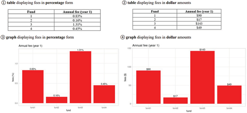
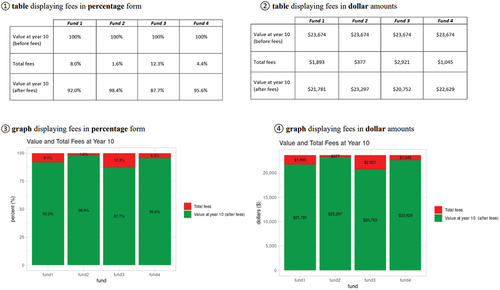
The difference between the two experiments is the way the fee information is presented. Experiment 1 displays the fees in either dollars or percentages using simple tables and bar charts (Panel A of Appendix 1A) based on one-year of fees. Experiment 2 displays the fees associated with the funds in terms of an ending balance (Panel B of Appendix 1A) based on ten-year fees. Experiment 2 is motivated by the Newall and Parker (2019) finding of improved decision-making when fees are converted from annual to ten-year equivalents.

2.1.1. Subjects

We recruited a sample of 448 crowdsourcing subjects from Amazon Mechanical Turk using CloudResearch (Chandler et al., 2019; Palan & Schitter, 2018) for both experiments. Appendix 2A discusses how the sample size was determined. The average time for the researchers to read the survey instrument was 2 minutes and 44 seconds. Any subject that completed the survey instrument in less than 2 minutes and 44 seconds was excluded. We included an attention-check question that asked, “Which of the following is NOT a shape?” The options were “circle,” “square,” “blue,” and “triangle.” Subjects that did not select “blue” as the answer were removed from the analysis based on best practices for using MTurk subjects (Aguinis et al., 2021).

2.1.2. Experimental materials

The materials place the subjects in the position of an individual investor who has $10,000, which must be invested in their personal portfolio. Subjects are informed that they will be presented some information about four index funds and then will be asked to make a judgment about how they would allocate $10,000 into those four index funds. The first manipulated variable, the presentation format (table vs. graph), was designed to test the effect of varying levels of visual formats on investor allocations. The second manipulated variable, unit of measurement ($ vs. %), was designed to test the effect of varying levels of these two measurement frames on investor allocations.¹

2.2. Experiment 1

2.2.1. Subjects

Experiment 1 consisted of 379 subjects. A total of 69 participants were excluded from Experiment 1 in the final analysis due to either completing the survey instrument too quickly or not passing an attention check. Eighteen subjects did not respond to the manipulation check, and 36% (128 of the total 360 manipulation check responses) correctly identified their presentation format when the manipulation check was performed.

The mean age of subjects in Experiment 1 was 42. A total of 62% of the subjects were female and 38% of the subjects were male. Out of these, 30% of the subjects had completed high school and 37% had an associate degree or higher.

2.2.2. Analysis of minimizing fees

According to past research on index funds, “In instances where fees differ, the only economically rational behavior is to make a 100% allocation to the lowest fee fund” (Mauck & Salzsieder, 2017, p. 49). Table 1 shows the proportion of subjects that minimized fees for all treatments.

Table 1. Fee minimization

Treatments			Minimized fees
Presentation format	Measurement level	n	n	%
table	%	94	16	17
table	$	100	12	12
graph	%	91	10	11
graph	$	94	10	11

In Table 2, Panel A, we report the mean amount allocated to each fund by treatment. On average, subjects allocated more money to the lowest fee fund (fund 2) versus the other funds. On average, for all treatments except the graph/dollar level, subjects allocated more money to the lowest fee fund (fund 2) versus the other funds.

Table 2. Descriptive statistics and multiple testing results for Experiment 1

Panel A: Average amount allocated to each fund by treatment.
Treatments						Average allocation
Presentation format		Measurement level		n		Fund 1	Fund 2		Fund 3		Fund 4
table		%		94		1925.96	3673.40		2089.50		2311.14
table		$		100		2338.30	3446.43		1938.48		2276.79
graph		%		91		2000.00	2982.97		2647.25		2369.78
graph		$		94		2545.84	2638.48		2690.10		2125.59
Panel B: Two-sided and one-directional (greater than) adjusted pairwise comparisons among treatment means
t-statistic adjusted p-value (two-sided test) adjusted p-value (one-sided)
Alternative Hypothesis		Treatment 1 (table, %)		Treatment 2 (table, $)		Treatment 3 (graph, %)			Treatment 4 (graph, $)
${\mu }_{Fund2}\ne {\mu }_{Fund1}$ ${\mu }_{Fund2}>{\mu }_{Fund1}$		4.12 (0.0012)* (0.0011)*		2.66 (0.0595) (0.0252)*		2.36 (0.1164) (0.0485)*			0.22 (1.0000) (0.4534)
${\mu }_{Fund2}\ne {\mu }_{Fund3}$ ${\mu }_{Fund2}>{\mu }_{Fund3}$		3.63 (0.0040)* (0018)*		4.06 (0.0012)* (0.0011)*		0.75 (1.0000) (0.4534)			0.12 (**) (1.0000)
${\mu }_{Fund2}\ne {\mu }_{Fund4}$ ${\mu }_{Fund2}>{\mu }_{Fund4}$		3.13 (0.0189)* (0.0080)*		2.90 (0.0336)* (0.0147)*		1.47 (0.7145) (0.2856)			1.28 (0.8116) (0.3045)

*significant at the 0.05 level

**this test was not performed since the mean amount allocated to fund 3 for this treatment was more than the mean amount allocated to the lowest fee fund (fund 2).

Even if subjects did not make an optimal decision and allocate 100% of funds to the lowest fee fund, we expect most allocations to be skewed towards the lowest fee fund (Fund 2). A many-to-one multiple comparison analysis of treatment means is presented in Table 2, Panel B. This analysis performed two-sided and one-sided t-tests. The one-sided tests allow for testing if the mean amount allocated to the lowest fee fund is significantly greater than the mean amount allocated to all other funds across the different treatments. Since the goal of this multiple testing is to identify treatments with a significantly “better” outcome (that is, on average, more money allocated to the lowest fee fund), a one-sided test, in addition to the two-sided test, is appropriate (Rafter et al., 2002).

It is common practice to adjust the p-values in the presence of multiple comparison tests to reduce the Type I error rate (Benjamini & Hochberg, 1995; Lee & Lee, 2018). While the Bonferroni correction is used extensively in many disciplines, it is not always the most appropriate p-value adjustment (Blakesley et al., 2009; Carmer & Swanson, 1973; Castaiieda et al., 1993; Félix & Menezes, 2018). Whether or not to use the Bonferroni correction depends on the circumstances of the research study (Armstrong, 2014). Some studies have suggested that the Bonferroni method should be used when the number of multiple tests is small, that is, 5 tests or less (Bender & Lange, 2001). The main disadvantage of using the Bonferroni adjustment is that it reduces the power of the statistical tests (Armstrong, 2014; Nakagawa, 2004; Olejnik et al., 1997). Since this study will perform more than 5 multiple tests and keeping the power of the statistical tests is important, this study will employ the Holm p-value correction (commonly referred to as the Bonferroni-Holm procedure) (Holm, 1979). The Holm adjustment has been shown to be as effective as the Bonferroni correction and increases statistical power (Abdi, 2010; Aickin & Gensler, 1996; Eichstaedt et al., 2013).

The multiple comparison tests displayed in Table 2 Panel B indicate that, on average, the amount allocated to the lowest fee fund is significantly different from all the other funds for treatments using a table, except for the table/dollar level. However, the table/dollar level is quite close to being significant at the 0.05 level of significance. The multiple comparison tests also indicate that the mean amount allocated to the lowest fee fund is significantly greater than the average amount allocated to all other funds for all treatments that contained a table, regardless of the unit of measurement. Only one of the treatments with a graph (graph, %) resulted in the mean amount allocated to the lowest fee fund being significantly greater than the mean amount allocated to fund 1.

These results suggest that regardless of the unit of measurement, displaying the fees in a table form leads to more money being allocated to the lowest fee fund rather than presenting the fees in a simple bar chart based on the one-sided tests.

2.2.3. Analysis of the optimal allocation

Table 3 shows how the subjects allocated the $10,000 among the funds for each treatment. Overall, only 13% (48 of 379) allocated the entire $10,000 to the lowest fee fund (minimized fees). Overwhelmingly, across all treatments, subjects diversified their money (bold row in Table 3) by selecting multiple funds. Our results are consistent with Scholl and Fontes (2022) who find that only 14% of participants in their survey were able to correctly calculate fees. Subjects were specifically told in the “Key Points to Remember” and “Frequently Asked Questions” introductory sections of both experiments that mutual funds have fees associated with them that lower investment returns (Appendix 3A). This result illustrates the desire for subjects to diversify even when it is not financially beneficial. Indeed, in an untabulated analysis regarding a qualitative question asking participants why they made the allocation that they did, the most common category of answers was related to a desire to diversify.

Table 3. Allocation of the $10,000 among the four fund choices

Treatment
# subjects that allocated	table, percentage n (%)		table, dollar n (%)	graph, percentage n (%)	graph, dollar n (%)	Total
all $10,000 to fund 1	3 (3.2%)		6 (6%)	5 (5.5%)	7 (7.4%)	21
all $10,000 to fund 2	16 (17%)		12 (12%)	10 (11%)	10 (10.6%)	48
all $10,000 to fund 3	3 (3.2%)		0 (0%)	5 (5.5%)	6 (6.4%)	14
all $10,000 to fund 4	3 (3.2%)		5 (5%)	4 (4.4%)	4 (4.3%)	16
$10,000 to two or more funds (diversified)	69 (73.4%)		77 (77%)	67 (73.6%)	67 (71.3%)	280
Total	94 (100%)		100 (100%)	91 (100%)	94 (100%)

To measure the extent to which the treatments affected the subjects’ propensity to engage in a naïve diversification strategy, Table 4 compares the concentration of funds by treatment, using a concentration measure based on the Euclidean distance from the perfectly even distribution (Beshears et al., 2011). This measure ranges from 0 ($2500 allocated equally across four funds) to $\sqrt{3/4}$ = 0.87 ($10,000 allocated entirely to a single fund) (Beshears et al., 2011). The mean concentration for all subjects was 0.45, with a standard deviation of 0.30. The average concentration values for all treatments are roughly halfway between 0 and 0.87. Therefore, the treatments applied to the subjects do not seem to lead the subjects to deviate from the naïve diversification strategy of equal allocations among the four funds.

Table 4. Average concentration measures by treatments

Treatment
	table, percentage mean (standard deviation)	table, dollar mean (standard deviation)	graph, percentage mean (standard deviation)	graph, dollar mean (standard deviation)
concentration	0.46 (0.29)	0.44 (0.29)	0.46 (0.29)	0.46 (0.30)

2.2.4. Analysis of post experimental questions

Table 5 shows how subjects rated the importance of various factors for their investment choices on a five-point Likert scale in the form of post-experimental questions (PEQs). The PEQs solicited responses about the subject’s self-identification of confidence in their allocation and the influence to diversify and minimize fees in their selection among their investment choices. There were five possible responses, from “not confident at all” to “extremely confident” for the confidence question, and “not at all influential” to “extremely influential” for the influence to minimize fees and diversify. Integer values 1 through 5 were assigned to each possible response, with higher integers corresponding to greater importance. The choice of a five-point scale for the confidence, desire to diversify, and minimize fees PEQs was based upon the Financial Management Behavioral Scale. All questions on this seminal survey related to financial behaviors use a five-point scale (Dew & Xiao, 2011). Responses with five to seven points have been shown to have higher reliability measures associated with them versus two to three points (Boateng et al., 2018). The majority of subjects ranked the middle category as “somewhat important/influential” as their response to the three PEQs. Sixty-seven percent of subjects reported they were somewhat confident, slightly confident, or not confident at all in their allocation decision. This result supports that accuracy and confidence are associated (Tekin & Roediger, 2017). For Experiment 1, most subjects were not confident in their allocation decision and most subjects were not accurate in their allocation decision. That is, most subjects did not select to allocate the entire $10,000 to the fund with the minimum fee (see Table 3). For the questions with the influential Likert scale, 75% reported that a desire to diversify was either somewhat influential, slightly influential, or not influential at all. This self-reported result is a contradiction of the decisions the subjects made in Experiment 1. Table 3 displays how most subjects did diversify the $10,000. Lastly, 63% of subjects reported that minimizing fees was either somewhat influential, slightly influential, or not at all influential. Table 3 supports this self-reporting statistic due to most subjects not selecting the fund with the minimum fee.

Table 5. Subject’s self-reported responses to PEQs

	Confidence How confident are you in your index mutual fund allocation decision?	Desire to diversify How much influence did a desire to diversify your investments have on your investment allocation decision?	Minimize fees How much influence did a desire to minimize fees have on your investment allocation decision?
	n (%)	n (%)	n (%)
Not confident at all Slightly confident	47 (12) 82 (22)
Somewhat confident Moderately confident Extremely confident	127 (34) 70 (19) 52 (13)
Not at all influential		69 (18)	48 (13)
Slightly influential		77 (20)	79 (21)
Somewhat influential		138 (37)	110 (29)
Very influential		65	75
Extremely influential		(17) 29 (7)	(20) 66 (17)

The PEQs were also analyzed based upon which subjects minimized fees and those who diversified. The one-way ANOVA (Analysis of Variance) test was performed to compare subjects’ fee minimization and the PEQs. Applying parametric statistical tests to Likert-scale data is more robust than applying non-parametric tests, even when normality assumptions are grossly violated (Norman, 2010). Recommendations from the literature suggest that when a Likert scale has five or more categories, the scale can be considered continuous (Harpe, 2015).

Table 6 displays the descriptive statistics for the PEQs and the results of the one-way ANOVA test. A one-way ANOVA revealed there was a statistically significant difference in the mean responses to the PEQ related to the desire to diversify between the subjects who did and did not minimize fees (i.e., diversified). This result indicates that subjects who realized there was no benefit to diversifying over multiple funds self-reported that diversifying was not as important to them (mean of 1.7 vs. 2.4).

Table 6. One-way ANOVA for the PEQs

	Minimized fees (all $10,000 to the lowest fee fund)	Diversified (allocated $10,000 to two or more funds)
Question	mean standard deviation	mean standard deviation	F (p-value)
Confidence	3.1 1.4	3.0 1.2	0.88 (0.3484)
Desire to diversify	1.7 0.9	2.4 0.8	22.36 (<0.0001)
Minimize fees	2.8 0.4	2.6 0.5	1.55 (0.2153)

It is interesting to note that the subjects that diversified did not rank, on average, that diversification was very important to them, with a mean of 2.4. However, it is somewhat counterintuitive to see that the mean influence of minimizing fees between both groups is not statistically significant. This result indicates that even among those that did minimize fees, the influence of the desire to minimize fees was no different from those who diversified. These results indicate that more work is needed to better understand why subjects are not minimizing fees when it is in their best interest to do so. One potential explanation is the Scholl and Fontes (2022) finding that roughly 80% of individual investors lack the knowledge to invest in mutual funds.

2.3. Experiment 2

2.3.1. Subjects

Experiment 2 consisted of 384 subjects. A total of 64 participants were excluded from Experiment 2 in the final analysis due to either completing the survey instrument too quickly or not passing an attention check. A total of 33 subjects did not respond to the manipulation check, and 41% (143 of the total 351 manipulation check responses) correctly identified their presentation format when the manipulation check was performed.

The mean age of subjects in Experiment 2 was 42. A total of 62% of the subjects were female and 38% of the subjects were male. A total of 29% of the subjects had completed high school and 42% had an associate degree or higher.

2.3.2. Analysis of minimizing fees

As in Table 1 for Experiment 1, Table 7 shows the proportion of subjects that minimized fees for all treatments in Experiment 2.

Table 7. Fee minimization

Treatments			Minimized fees
Presentation format	Measurement level	n	n	%
table	%	88	25	28
table	$	92	27	29
graph	%	103	15	15
graph	$	101	21	21

In Table 8 Panel A, we report the mean amount allocated to each fund by treatment. On average, subjects allocated more money to the lowest fee fund (fund 2) versus the other funds. On average, for all treatments, subjects allocated more money to the lowest fee fund (fund 2) than to the other funds.

Table 8. Descriptive statistics and multiple testing results for Experiment 2

Panel A: Average amount allocated to each fund by treatment.
Treatments					Average allocation
Presentation format	Measurement level		n		Fund 1		Fund 2	Fund 3		Fund 4
table	%		88		1977.38		4939.18	1405.78		1677.66
table	$		92		2296.74		4802.42	1203.93		1696.90
graph	%		103		2059.03		4128.16	1733.69		2079.13
graph	$		101		1865.01		4354.54	1677.23		2103.22
Panel B: Two-sided and One-directional (greater than) adjusted pairwise comparisons among treatment means
t-statistic adjusted p-value (two-sided) adjusted p-value (one-sided)
Alternative Hypothesis		Treatment 1 (table, %)		Treatment 2 (table, $)		Treatment 3 (graph, %)			Treatment 4 (graph, $)
${\mu }_{Fund2}\ne {\mu }_{Fund1}$ ${\mu }_{Fund2}>{\mu }_{Fund1}$		6.19 (0.0004)* (0.0004)*		5.06 (0.0004)* (0.0004)*		5.44 (0.0004)* (0.0004)*			5.88 (0.0004)* (0.0004)*
${\mu }_{Fund2}\ne {\mu }_{Fund3}$ ${\mu }_{Fund2}>{\mu }_{Fund3}$		8.13 (0.0004)* (0.0004)*		8.26 (0.0004)* (0.0004)*		6.80 (0.0004)* (0.0004)*			6.46 (0.0004)* (0.0004)*
${\mu }_{Fund2}\ne {\mu }_{Fund4}$ ${\mu }_{Fund2}>{\mu }_{Fund4}$		7.44 (0.0004)* (0.0004)*		7.01 (0.0004)* (0.0004)*		5.97 (0.0004)* (0.0004)*			5.58 (0.0004)* (0.0004)*

*significant at the 0.05 level

The multiple comparison tests displayed in Table 8 Panel B are all significant for both the one-sided and two-sided tests. The raw p-values from the tests were adjusted similarly to Experiment 1. All the raw p-values from the one-sided and two-sided tests were<0.0001. A p-value of 0.0001 was used when the adjustment was made, which resulted in an adjusted p-value of 0.0004 for all tests. Since all the adjusted p-values are same, an analysis of the magnitude of the t-statistics is useful to determine where the largest difference (standardized difference) between the mean amount allocated to the lowest fee fund (fund 2) and the other funds exists. The larger the t-statistic indicates that more money, on average, was allocated to fund two versus the other funds. The two largest t-statistics are associated with the treatments that consisted of a table with either unit of measurement, with the dollar unit of measurement being slightly higher. The majority of the larger t-statistics are associated with the treatments that contained tables. Again, these results suggest that displaying the fees in a table form leads subjects to allocate more, on average, to the lowest fee fund when compared to other funds across the different treatment levels.

2.3.3. Analysis of the optimal allocation

Table 9 shows how the subjects allocated the $10,000 among the funds for each treatment. Overall, only 23% (88 of 379) allocated the entire $10,000 to the lowest fee fund (minimized fees). Overwhelmingly, again with Experiment 2, across all treatments, subjects diversified their money (bold row in Table 9). This result from Experiment 2 illustrates the desire for subjects to diversify even when it is not financially beneficial.

Table 9. Allocation of the $10,000 among the four fund choices

Treatment
# subjects that allocated	table, percentage n (%)	table, dollar n (%)	graph, percentage n (%)	graph, dollar n (%)	Total
all $10,000 to fund 1	5 (5.7%)	7 (7.6%)	1 (0.9%)	4 (4.0%)	17
all $10,000 to fund 2	25 (28.4%)	27 (29.3%)	15 (14.6%)	21 (20.8%)	88
all $10,000 to fund 3	0 (0%)	1 (0%)	1 (0.9%)	3 (3.0%)	5
all $10,000 to fund 4	1 (1.1%)	1 (1.1%)	0 (0%)	1 (0.9%)	3
$10,000 to two or more funds (diversified)	57 (64.7%)	56 (60.9%)	86 (83.5%)	72 (71.3%)	271
Total	88 (100%)	92 (100%)	103 (100%)	101 (100%)

Table 10 compares the concentration of funds by treatment, using a concentration measure explained for Experiment 1. The mean concentration for all subjects was 0.46, with a standard deviation of 0.31. The lowest concentration value corresponds to the graph/percentage treatment. This treatment seems to have the least effect on moving subjects away from naïve diversification behavior. This effect can also be observed in Table 9. The graph/percentage treatment has the highest percentage of subjects that diversified their funds. Similarly, as in Experiment 1, the concentration measures for the other treatments are roughly halfway between 0 and 0.87. Therefore, the treatments applied to the subjects do not seem to lead the subjects to deviate from the naïve diversification strategy of equal allocations among the four funds.

Table 10. Concentration measures by treatments

Treatment
	table, percentage mean (standard deviation)	table, dollar mean (standard deviation)	graph, percentage mean (standard deviation)	graph, dollar mean (standard deviation)
concentration	0.49 (0.31)	0.50 (0.30)	0.39 (0.30)	0.48 (0.30)

2.3.4. Analysis of post experimental questions

Table 11 shows how subjects rated the importance of various factors for their investment choices in a similar manner as described in Experiment 1. As in Experiment 1, the majority of subjects ranked the middle category “somewhat important/influential” as their response to all three PEQs. The self-reported results of the PEQs for Experiment 2 is similar to Experiment 1. Sixty-three percent of subjects reported they were somewhat confident, slightly confident, or not confident at all in their allocation decision. For Experiment 2, most subjects were not confident in their allocation decision and most subjects did not select to allocate the entire $10,000 to the fund with the minimum fee (see Table 9). For the questions with the influential Likert scale, 74% reported that a desire to diversify was either somewhat influential, slightly influential, or not influential at all. This self-reported result is a contradiction of the decisions the subjects made in Experiment 2. Table 9 displays how most subjects did diversify the $10,000. Fifty percent of subjects reported that minimizing fees was either somewhat influential, slightly influential, or not at all influential. This statistic is less than the self-reported statistic from Experiment 1. The lower self-reported minimizing fees percentage in Experiment 2 may be supported by the fact that more subjects did allocate all $10,000 to the lowest fee fund compared to Experiment 1.

Table 11. Subject’s self-reported responses to PEQs

	Confidence How confident are you in your index mutual fund allocation decision?	Desire to diversify How much influence did a desire to diversify your investments have on your investment allocation decision?	Minimize fees How much influence did a desire to minimize fees have on your investment allocation decision?
	n (%)	n (%)	n (%)
Not confident at all Slightly confident	39 (10) 74 (19)
Somewhat confident Moderately confident Extremely confident	127 (33) 83 (22) 58 (15)
Not at all influential		83 (22)	34 (9)
Slightly influential		79 (21)	57 (15)
Somewhat influential		121 (32)	100 (26)
Very influential		62	98
Extremely influential		(16) 36 (9)	(26) 91 (24)

Table 12 displays the descriptive statistics for the PEQs and the results of the one-way ANOVA test for Experiment 2. A one-way ANOVA revealed there were statistically significant differences in the PEQs related to the confidence of the subject’s allocation and their desire to diversify between the subjects who did and did not minimize fees (i.e., diversified).

Table 12. One-way ANOVA for the PEQs

	Minimized fees (all $10,000 to the lowest fee fund)	Diversified (allocated $10,000 to two or more funds)
Question	mean standard deviation	mean standard deviation	F (p-value)
Confidence	3.4 1.3	3.1 1.1	5.39 (0.0208)
Desire to diversify	1.6 0.8	2.3 0.8	45.82 (<0.0001)
Minimize fees	2.7 0.5	2.6 0.5	0.05 (0.8304)

Interestingly, a significant difference was found with regard to confidence for Experiment 2. Panel of Appendix 2A shows how the graphs and tables were presented in Experiment 2. The graphs and tables used in Experiment 2 are more “complex” than those used in Experiment 1. By “more complex,” we mean more rows and columns in the tables and a stacke bar chart was used instead of a simple bar chart. In both groups (those that did and did not diversify), the confidence in the allocation decision is higher for Experiment 2 versus Experiment 1.

Similarly, as found in Experiment 1, it is somewhat counterintuitive to see that the mean influence of minimizing fees between both groups is not statistically significant. This result again indicates that even among those that did minimize fees, the influence of the desire to minimize fees was no different from those who did not minimize fees.

3. Results and discussion

As indicated by both the wide range of fees on S&P 500 Index Mutual Funds in the marketplace and experimental evidence, investors fail to minimize fees when selecting such funds. This behavior violates the Law of One Price, which indicates that commodity-like goods such as S&P 500 Index Mutual Funds should see convergence in fees. While this deviation from optimal behavior has been well-studied, there has been less focus on the interventions that may improve investor decision-making.

In this study, we extend a growing literature on the potential for information presentation to improve general decision-making. To our knowledge, no such effort has been made in the context of S&P 500 Index Mutual Funds. This product provides a context ideal for experimentation because, contrary to actively managed mutual funds and other similar investment products, all index funds will have identical future returns. As such, the optimal decision is knowable a priori, and investors should seek to minimize fees.

4. Conclusions

Our experiments yield some promising conclusions. The use of tables leads to better investment allocations than the use of graphs when displaying fee information. Further, providing fees based on their ten-year costs rather than one-year costs improves investor allocations. Yet, the results also indicate a need for considerable additional research given that even in the best-case scenarios of our experiments, the vast majority of participants fail to minimize fees and often allocate substantial amounts of money to the highest fee fund. Our results do not address possible causes of the continued failure to minimize fees, but a likely driver is the aforementioned lack of mutual fund understanding amongst individual investors (Scholl & Fontes, 2022). Finally, our experiments provided much less information than investors would be faced with in the real world. Despite the relatively simple disclosure and decision to be made, the average result is strongly suboptimal. Thus, it will be important to better understand why investors misallocate when selecting index mutual funds to better provide disclosures that lead to wealth-enhancing decisions for individual investors.

Disclosure statement

No potential conflict of interest was reported by the authors.

Notes

1. A manipulation check was structured as a multiple-choice question as follows: In the scenario that you just read and completed, how was the fee information presented to you? The subjects were provided a link that showed them the four possible treatments (panels A and B of Appendix 1). The instructions stated to close the window with the treatments and navigate back to the survey instrument and select the presentation format the subject was presented. The analyses in this study are based on responses from all subjects for both experiments, regardless of whether they passed the manipulation check or not (Aronow et al., 2019).

Appendices Appendix

Panel A: Four treatments for Experiment 1

Panel B: Four Treatments for Experiment 2

Appendix

Sample size determination allows researchers to conserve resources when designing a study and still achieve conclusive results. Sample size determination is decided upon before the study is conducted to ensure the researcher has enough data to obtain the results of the statistical test they wish to observe (Lenth, 2001). In the biomedical field, authors are expected to describe the sample size computations in sufficient detail to enable a knowledgeable reader with the original data to be able to verify the computations (Kang, 2021). It has been reported in the accounting discipline that more researchers need to conduct sample size studies for experiments (Kim et al., 2018). Another compelling reason to provide the details of a statistical design like sample size calculations is directly related to the reproducibility crisis that is occurring in many scientific disciplines (Al Rahahleh et al., 2019).

The authors of this study provide the details of the sample size analyses so that perhaps others in the behavioral and experimental finance disciplines will consider these statistical considerations for their experiments.

Sample size calculations are driven by five key factors: power (1-$\beta )$, effect size, significance level ($\alpha$), and the type of statistical analysis. In this study, the authors used the SAS procedure PROC GLMPOWER to compute the required sample size. PROC GLMPOWER is an appropriate SAS procedure for a 2 × 2 ANOVA model (Park, 2015).

Power (1-$\beta$) and Significance Level ($\alpha$)

Power can be examined through the lens of a hypothesis test. Below is the hypothesis test for the 2 × 2 ANOVA model for Experiment 1.

${\mathrm{H}}_0:{\mu }_{table,percentage}={\mu }_{table,dollars}={\mu }_{graph,percentage}={\mu }_{graph,dollars}$

H₁: not (${\mu }_{table,percentage}={\mu }_{table,dollars}={\mu }_{graph,percentage}={\mu }_{graph,dollars}$)

where $\mu$ is the average amount that the subjects allocate to the lowest fee fund.

H₀ is the null hypothesis and is a statement that there is no difference among the treatment means. H₁ is the alternative and is the opposite statement of the null hypothesis. In this case, the alternative is to test for at least one mean that is different from the others.

In hypothesis testing, you use a decision rule. The question now becomes was the decision made correctly?

Table A2.1 displays a schematic that shows the two types of decisions and the statistical consequences of those decisions.

Table A2.1. Consequences and decisions for statistical tests

Actual
	H0 is true	H0 is false
Decision
Reject H0	Correct (1-$\alpha )$=confidence	Error=$\beta$ Type II Error
Do not reject H0	Error=$\alpha$=level of significance Type I Error	Correct (1-$\beta$)=power

Using Table A2.1, power is defined when we reject the null hypothesis and the null is false. This is the correct decision, and we want as high of power as possible for a statistical test. In this study, a power of 80% was chosen. A power value of 80% is a standard choice for statistical tests (Ellis, 2010).

This study uses a level of significance ($\alpha$) of 0.05. The scientific community has a long history of using 0.05 as a standard for scientific inference (Kennedy-Shaffer, 2019; Manderscheid, 1965).

Effect size

The effect size is the difference in the mean response values among the different treatments that the researcher wishes to detect (O’brien & Castelloe, 2004). The effect size is determined by the hypothesized treatment means and standard deviations the researcher proposes. The hypothesized treatment means represent the desired possible scientific meaningful difference a researcher is willing to detect (High, 2007). These hypothesized means can be from past studies, the researcher’s own empirical experience, or what the researcher hypothesizes will be the results of the designed experiment. In this study, the researchers are hypothesizing the desired hypothetical results. Table A2.2 displays the hypothesized means the authors expect subjects will allocate to the lowest fund fee for each treatment combination.

Table A2.2. Hypothesized response means for the 2 × 2 ANOVA for Experiment 1

Factor 2 (unit of measurement)
Factor 1 (presentation format)	$	%
table	$6500	$4500
graph	$8500	$5500

Proc glmpower

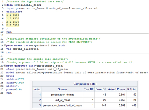
Figure A2.1 provides the SAS code used to determine the sample size for Experiment 1, along with the output from PROC GLMPOWER. The SAS output indicates that for this study to achieve a power of 80%, a sample size of 448 subjects is required.

Figure A2.1. SAS code and output to calculate the required sample size for Experiment 1.

Appendix 3A.

The following information was provided to all subjects in both experiments

References

- Abdi, H. (2010). Holm’s sequential Bonferroni procedure. Encyclopedia of Research Design, 1(8), 1–22.
- Aguinis, H., Villamor, I., & Ramani, R. S. (2021). Mturk research: Review and recommendations. Journal of Management, 47(4), 823–837. https://doi.org/10.1177/0149206320969787
- Aickin, M., & Gensler, H. (1996). Adjusting for multiple testing when reporting research results: The Bonferroni vs Holm methods. American Journal of Public Health, 86(5), 726–728. https://doi.org/10.2105/AJPH.86.5.726
- Al Rahahleh, N., & Bhatti, M. I. (2022). Empirical comparison of Shariah-compliant vs conventional mutual fund performance. International Journal of Emerging Markets. https://doi.org/10.1108/IJOEM-05-2020-0565
- Al Rahahleh, N., Bhatti, M. I., & Misman, M. N. (2019). Developments in risk management in Islamic finance: A review. Journal of Risk and Financial Management, 12(1), 37. https://doi.org/10.3390/jrfm12010037
- Anic, V., & Wallmeier, M. (2020). Perceived attractiveness of structured financial products: The role of presentation format and reference instruments. Journal of Behavioral Finance, 21(1), 78–102. https://doi.org/10.1080/15427560.2019.1629441
- Armstrong, R. A. (2014). When to use the Bonferroni correction. Ophthalmic and Physiological Optics, 34(5), 502–508. https://doi.org/10.1111/opo.12131
- Aronow, P. M., Baron, J., & Pinson, L. (2019). A note on dropping experimental subjects who fail a manipulation check. Political Analysis, 27(4), 572–589. https://doi.org/10.1017/pan.2019.5
- Ashraf, D., Khawaja, M., & Bhatti, M. I. (2022). Raising capital amid economic policy uncertainty: An empirical investigation. Financial Innovation, 8(1), 1–32. https://doi.org/10.1186/s40854-022-00379-w
- Bender, R., & Lange, S. (2001). Adjusting for multiple testing—when and how? Journal of Clinical Epidemiology, 54(4), 343–349. https://doi.org/10.1016/S0895-4356(00)00314-0
- Benjamini, Y., & Hochberg, Y. (1995). Controlling the false discovery rate: A practical and powerful approach to multiple testing. Journal of the Royal Statistical Society Series B (Methodological), 57(1), 289–300. https://doi.org/10.1111/j.2517-6161.1995.tb02031.x
- Beshears, J. L., Choi, J. J., Laibson, D. I., & Madrian, B. C. (2011). How does simplified disclosure affect individuals’ mutual fund choices? SSRN Journal University of Chicago Press, Chicago, 13, 75.
- Blakesley, R. E., Mazumdar, S., Dew, M. A., Houck, P. R., Tang, G., Reynolds, C. F., & Butters, M. A. (2009). Comparisons of methods for multiple hypothesis testing in neuropsychological research. Neuropsychology, 23(2), 255–264. https://doi.org/10.1037/a0012850
- Boateng, G. O., Neilands, T. B., Frongillo, E. A., Melgar-Quiñonez, H. R., & Young, S. L. (2018). Best practices for developing and validating scales for health, social, and behavioral research: A primer. Frontiers in Public Health, 6. https://doi.org/10.3389/fpubh.2018.00149
- Cardoso, R. L., Leite, R. O., Aquino, A. C. B. D., & García-Gallego, A. (2016). A graph is worth a thousand words: How overconfidence and graphical disclosure of numerical information influence financial analysts accuracy on decision making. PLoS One, 11(8), e0160443. https://doi.org/10.1371/journal.pone.0160443
- Carmer, S. G., & Swanson, M. R. (1973). An evaluation of ten pairwise multiple comparison procedures by Monte Carlo methods. Journal of the American Statistical Association, 68(341), 66–74. https://doi.org/10.1080/01621459.1973.10481335
- Castaiieda, M. B., Levin, J. R., & Dunham, R. B. (1993). Using planned comparisons in management research: A case for the Bonferroni procedure. Journal of Management, 19(3), 707–724. https://doi.org/10.1177/014920639301900311
- Chandler, J., Rosenzweig, C., Moss, A. J., Robinson, J., & Litman, L. (2019). Online panels in social science research: Expanding sampling methods beyond mechanical Turk. Behavior Research Methods, 51(5), 2022–2038. https://doi.org/10.3758/s13428-019-01273-7
- Choi, J. J., Laibson, D., & Madrian, B. C. (2010). Why does the law of one price fail? An experiment on index mutual funds. The Review of Financial Studies, 23(4), 1405–1432. https://doi.org/10.1093/rfs/hhp097
- DeSanctis, G. (1984). Computer graphics as decision aids: Directions for research. Decision Sciences, 15(4), 463–487. https://doi.org/10.1111/j.1540-5915.1984.tb01236.x
- Dew, J., & Xiao, J. (2011). The financial management behavior scale: Development and validation. Financial Counseling and Planning, 22(1), 43.
- Eberhard, K. (2021). The effects of visualization on judgment and decision-making: A systematic literature review. Management Review Quarterly, 73(1), 167–214. https://doi.org/10.1007/s11301-021-00235-8
- Eichstaedt, K. E., Kovatch, K., Maroof, D. A., Greenwald, B. D., & Gurley, J. M. (2013). A less conservative method to adjust for familywise error rate in neuropsychological research: The Holm’s sequential Bonferroni procedure. NeuroRehabilitation, 32, 693–696. https://doi.org/10.3233/NRE-130893
- Ellis, P. D. (2010). The essential guide to effect sizes: Statistical power, meta-analysis, and the interpretation of research results. Cambridge University Press.
- Félix, V., & Menezes, A. (2018). Comparisons of ten corrections methods for t-test in multiple comparisons via Monte Carlo study. The Electronic Journal of Applied Statistical Analysis, 11(1), 74–91.
- Guo, X., Liang, C., Umar, M., & Mirza, N. (2022). The impact of fossil fuel divestments and energy transitions on mutual funds performance. Technological Forecasting and Social Change, 176, 121429. https://doi.org/10.1016/j.techfore.2021.121429
- Harcourt-Cooke, C., Els, G., & van Rensburg, E. (2022). Using comics to improve financial behaviour. Journal of Behavioral and Experimental Finance, 33, 100614. https://doi.org/10.1016/j.jbef.2021.100614
- Harpe, S. E. (2015). How to analyze Likert and other rating scale data. Currents in Pharmacy Teaching and Learning, 7(6), 836–850. https://doi.org/10.1016/j.cptl.2015.08.001
- Harvey, N., & Bolger, F. (1996). Graphs versus tables: Effects of data presentation format on judgemental forecasting. International Journal of Forecasting, 12(1), 119–137. https://doi.org/10.1016/0169-2070(95)00634-6
- High, R. (2007, September 17). Introduction to statistical power calculations for linear models with SAS 9.1. Retrieved June, 13, 2011.
- Holm, S. (1979). A simple sequentially rejective multiple test procedure. Scand J Stat, 6(2), 65–70.
- Huang, J., Wei, K. D., & Yan, H. (2022). Investor learning and mutual fund flows. Financial Management, 51(3), 739–765. https://doi.org/10.1111/fima.12378
- Iannotta, G., & Navone, M. (2012). The cross-section of mutual fund fee dispersion. Journal of Banking & Finance, 36(3), 846–856. https://doi.org/10.1016/j.jbankfin.2011.09.013
- Isler, O., Rojas, A., & Dulleck, U. (2022). Easy to shove, difficult to show: Effect of educative and default nudges on financial self-management. Journal of Behavioral and Experimental Finance, 34, 100639. https://doi.org/10.1016/j.jbef.2022.100639
- Kang, H. (2021). Sample size determination and power analysis using the G*Power software. Journal of Educational Evaluation for Health Professions, 18, 17. https://doi.org/10.3352/jeehp.2021.18.17
- Kennedy-Shaffer, L. (2019). Before p < 0.05 to beyond p < 0.05: Using history to contextualize p-values and significance testing. The American Statistician, 73(sup. 1), 82–90. https://doi.org/10.1080/00031305.2018.1537891
- Kim, J. H., Ahmed, K., & Ji, P. I. (2018). Significance testing in accounting research: A critical evaluation based on evidence: SIGNIFICANCE TESTING. Abacus, 54(4), 524–546. https://doi.org/10.1111/abac.12141
- Lee, S., & Lee, D. K. (2018). What is the proper way to apply the multiple comparison test? Korean Journal of Anesthesiology, 71(5), 353–360. https://doi.org/10.4097/kja.d.18.00242
- Lenth, R. V. (2001). Some practical guidelines for effective sample size determination. The American Statistician, 55(3), 187–193. https://doi.org/10.1198/000313001317098149
- Manderscheid, L. V. (1965). Significance levels. 0.05, 0.01, Or? Journal of Farm Economics, 47(5), 1381–1385. https://doi.org/10.2307/1236396
- Mansor, F., Bhatti, M. I., & Ariff, M. (2015). New evidence on the impact of fees on mutual fund performance of two types of funds. Journal of International Financial Markets, Institutions and Money, 35, 102–115. https://doi.org/10.1016/j.intfin.2014.12.009
- Mauck, N., & Salzsieder, L. (2017). Diversification bias and the law of one price: An experiment on index mutual funds. Journal of Behavioral Finance, 18(1), 45–53. https://doi.org/10.1080/15427560.2017.1276067
- Ma, Y., Xiao, K., Zeng, Y., & Koijen, R. (2022). Mutual fund liquidity transformation and reverse flight to liquidity. The Review of Financial Studies, 35(10), 4674–4711. https://doi.org/10.1093/rfs/hhac007
- Nakagawa, S. (2004). A farewell to Bonferroni: The problems of low statistical power and publication bias. Behavioral Ecology, 15(6), 1044–1045. https://doi.org/10.1093/beheco/arh107
- Newall, P. W. S., & Love, B. C. (2015). Nudging investors big and small toward better decisions. Decision, 2(4), 319–326. https://doi.org/10.1037/dec0000036
- Newall, P. W. S., & Parker, K. N. (2019). Improved mutual fund investment choice architecture. Journal of Behavioral Finance, 20(1), 96–106. https://doi.org/10.1080/15427560.2018.1464455
- Norman, G. (2010). Likert scales, levels of measurement and the “laws” of statistics. Advances in Health Sciences Education, 15(5), 625–632. https://doi.org/10.1007/s10459-010-9222-y
- O’brien, R., & Castelloe, J., 2004. Sample-size analysis in study planning: Concepts and issues, with examples using. Proc Power and Proc. GLMPOWER. Proc. SUGI 29 Conference. Montreal, Canada.
- Olejnik, S., Li, J., Supattathum, S., & Huberty, C. J. (1997). Multiple testing and statistical power with modified Bonferroni procedures. Journal of Educational and Behavioral Statistics, 22(4), 389–406. https://doi.org/10.3102/10769986022004389
- Palan, S., & Schitter, C. (2018). Prolific.Ac—a subject pool for online experiments. Journal of Behavioral and Experimental Finance, 17, 22–27. https://doi.org/10.1016/j.jbef.2017.12.004
- Park, H. M., 2015. Hypothesis testing and statistical power of a test. https://scholarworks.iu.edu/dspace/handle/2022/19738.
- Rafter, J. A., Abell, M. L., & Braselton, J. P. (2002). Multiple comparison methods for means. SIAM Review, 44(2), 259–278. https://doi.org/10.1137/S0036144501357233
- Rosdini, D., Sari, P. Y., Amrania, G. K. P., & Yulianingsih, P. (2020). Decision making biased: How visual illusion, mood, and information presentation plays a role. Journal of Behavioral and Experimental Finance, 27, 100347. https://doi.org/10.1016/j.jbef.2020.100347
- Scholl, B., & Fontes, A. (2022). Mutual fund knowledge assessment for policy and decision problems. Financial Services Review, 30(1), 31–56.
- Tekin, E., & Roediger, H. L. (2017). The range of confidence scales does not affect the relationship between confidence and accuracy in recognition memory. Cognitive Research: Principles and Implications, 2(1), 49. https://doi.org/10.1186/s41235-017-0086-z