An investigation of financial contagion between cryptocurrency and equity markets: Evidence from developed and emerging markets

Abstract

The present study conducts a dynamic conditional cross-correlation and time–frequency correlation analyses between cryptocurrency and equity markets in both advanced and emerging economies. The purpose of the study is twofold. First, the study investigates the presence of the pure (narrow) form of financial contagion between cryptocurrency and stock markets in both advanced and emerging economies, during the black swan event of the COVID-19 crisis. Second, the study examines the hedging and safe-haven properties of cryptocurrencies against equity markets, before and during periods of financial upheaval triggered by the COVID-19 pandemic. Two econometric models are used: (1) the dynamic conditional correlation (DCC) GARCH and (2) the wavelet analysis models. Using the DCC GARCH model, the study found the evidence of high conditional correlations between cryptocurrency and equity markets. The high conditional correlation was mostly detected in periods of financial turmoil corresponding to the first quarter and the second quarter of 2020. The increase in conditional correlation during periods of financial upheaval (compared to a tranquil period) indicates the presence of the pure form of financial contagion. The wavelet cross-correlation analysis showed the evidence of positive cross-correlation between the Bitcoin and the equity markets during period of financial turmoil. The cross-correlation was identified in both short and long (coarse) scales. In short scales, the equity markets lead the cryptocurrency market, while the cryptocurrency market leads equity markets in coarse scales. The findings of the present study revealed that the degree of interdependence between cryptocurrency and equity markets has substantially increased during the COVID-19 period, and this has negated the safe-haven and hedging benefits of cryptocurrencies over equity markets.

Keywords:

• COVID-19
• cryptocurrency
• DCC GARCH
• equity market
• financial contagion
• wavelet analysis

Public Interest Statement

This study examined the relationship between cryptocurrency and stock markets, in advanced and emerging economies, during the COVID-19 crisis. The study also investigated whether or not cryptocurrencies could act as a safe-haven asset during times of financial stress. A safe-haven asset is an investment that is expected to hold its value or even increase in value during times of economic or political uncertainty. The study found that there was a high correlation between cryptocurrency and stock markets (in advanced and emerging economies) during periods of financial turmoil caused by COVID-19 pandemic. The study conclude that cryptocurrencies may not be as reliable as a safe-haven investment during times of financial instability.

1. Introduction

The value and popularity of cryptocurrencies have been increasing dramatically in recent years. Bitcoin, one of the leading and most liquid cryptocurrencies, has seen its price soar to record-breaking heights since its inception in 2008 by the developer operating under the pseudonym Satoshi Nakamoto (Biju et al., 2022). While advanced economies such as the USA are among the most technologically prepared for the adoption of crypto assets, emerging market economies have recently shown strong adoption of these assets, with nine of the top 10 big adopters in 2021 being from emerging markets (Iyer, 2022).

Due to their independence from momentary policies and apparent low correlation with traditional assets, cryptocurrencies have been touted as a good hedge against inflation and a safe-haven when the stock market slumps. This has led to them being dubbed the “digital gold” (Huynh et al. (2021). However, the COVID-19 pandemic appears to have negated the diversification and hedging benefits of cryptocurrencies. Research has demonstrated that during the COVID-19 period, the correlation between crypto assets and traditional holdings such as stocks has significantly increased.¹

It is against this background that the current study examines the pure (narrow) form of financial contagion between cryptocurrency and both developed and emerging equity markets, during the crisis caused by the COVID-19 pandemic. A financial contagion is defined as the spread of an economic crisis from one market or region to another due to factors that cannot be explained by economics fundamentals and are solely the result of irrational phenomena, such as panics, herd behaviour, loss of confidence, and risk aversion. Financial contagion happens if the correlation intensifies during the period of financial turmoil. If the co-movement does not intensify considerably during the period of financial upheaval, then any persistent high level of market correlation suggests only strong linkages between the two markets or economies, commonly referred to as interdependence. As previously mentioned, the recent adoption of cryptocurrencies has been particularly pronounced in emerging market countries, with emerging market economies accounting for nine of the top 10 significant adopters in 2021 (Iyer, 2022).

It is also worth noting that there is a paucity of literature that attempts to investigate the correlation between cryptocurrencies with stock market returns especially in emerging economies markets. A review of existing studies by the researchers found that the study conducted by Shahzad et al. (2022) is the most closely related paper to the current study. Shahzad et al. (2022) examined the interconnectedness and interdependencies of Bitcoin, gold, and US VIX futures to evaluate their hedging abilities against downside movements in BRICS stock market indices. The authors concluded that gold, rather than Bitcoin, demonstrated greater and more consistent diversification advantages in China, especially during the COVID-19 pandemic. On the other hand, VIX futures appeared to offer enhanced diversification benefits in Brazil, Russia, India, and South Africa during the COVID-19 crisis, unlike Bitcoin. Shahzad et al. (2022) only focused on the BRICS stock market. The present study builds on the work of Shahzad et al. (2022) by examining the relationship between cryptocurrencies and stock market returns in a broader context. Additionally, the findings of Shahzad et al. (2022) suggested that the diversification benefits of different alternative assets may vary across countries and during different market conditions. The current study aims to further investigate this relationship by using MSCI and S&P500 as proxies for emerging markets and advanced markets, respectively, to provide a more comprehensive understanding of the potential correlations between cryptocurrencies and stock market returns in different economies.

Our results show that there is a positive cross-correlation between the cryptocurrency and the equity markets during the period of financial turmoil caused by COVID-19. A positive high correlation during the period of turbulence (compare to stable periods) is indicative of the presence of the pure form of financial contagion between the two markets. The lead-lag analysis also revealed that in short- and medium-term horizon the equity markets (in both advanced and emerging economies) lead the cryptocurrency market, while the cryptocurrency market leads equity markets in long-term horizon. A positive cross-correlation (in-phase) relationship between the two market implies that there are reduced benefits of portfolio diversification and hedging strategies. The conclusion is that hedging strategies that would normally work under normal market conditions are prone to fail during the periods of financial/economic upheaval. Put simply cryptocurrency should not be used as a safe-haven during episodes of high volatility.

This section is an introduction. The rest of the paper is arranged as follow: Section 2 reviews the literature on volatility of cryptocurrencies and the spillover effects on other markets. In Section 3, the methodology used in the paper is outlined, whereas Section 4 presents the results from our analysis and also discusses these results in the context of the previous literature and the objectives of this paper. Section 5 concludes the paper, and Section 6 provides recommendations.

2. Literature review

Cryptocurrencies allow for the exchange of financial resources outside the regulated financial system. The blockchain technology on which these virtual currencies are based enables peer-to-peer transactions without the need for an intermediary or central bank backstop. While this makes the system susceptible to abuse by hackers, it is also cheaper to use compared to traditional banking systems. The advantage of using cryptocurrencies is their ability to facilitate transactions away from regulatory-imposed inefficiencies, transaction costs, and time delays created by intermediaries (Corbet et al, 2019; Naimy et al., 2021). In addition to the decentralised nature of crypto markets, high trading volumes have significantly ensured high liquidity, implying high efficiency in crypto markets compared to traditional financial markets. An increased number of cryptocurrencies since the introduction of Bitcoin in 2008 has provided investors with alternative diversification instruments (Lucey et al., 2022).

There has been a renewed interest in volatility analysis in recent years, with a particular focus on cryptocurrencies (Bhosale & Mavale, 2018; Naimy et al., 2021; Saleh, 2019). Mainly two strands of literature analysing the volatility of crypto markets emerge from available studies. The first line of inquiry focuses on the volatility of and between different kinds of cryptocurrencies, and the second strand of literature examines volatility spillovers between cryptocurrencies and traditional asset classes. These two areas of research provide insights into the volatility dynamics of cryptocurrencies in different contexts and contribute to our understanding of their behaviour in financial markets.

In the first strand of literature, scholars focused on the volatility of and between different kinds of cryptocurrencies (Kumar & Anandarao, 2019; Fakhfekh & Jeribi, 2020; Saleh, 2019). This literature provides evidence of the high volatility in crypto markets compared to traditional financial markets. While this adds to our understanding of these new markets in general, the information provided is of particular interest to investors intending to add these assets to their portfolios or those already holding such assets in their portfolios. Available research points to a general consensus that cryptocurrencies offer high returns but also carry high risk (Iyer, 2022; Naimy et al., 2021). Additionally, cryptocurrencies are found to exhibit market inefficiency and long memory (Kumar & Anandarao, 2019; Salisu & Ogbonna, 2021). Begušić et al. (2018) argue that the presence of fat tails and a finite second moment for Bitcoin returns signals the applicability of mainstream financial theories and analysis.

In addition to analysing the nature of volatility in cryptocurrencies, there have been studies that investigated the volatility dynamics among different types of cryptocurrencies. For instance, Gupta and Chaudhary (2022) conducted research on the relationship between the return and return volatility of four commonly traded cryptocurrencies. Their findings revealed a strong spillover effect between Bitcoin and Ether, as well as an asymmetric impact between Litecoin and XRP. In another study, Kumar et al. (2022) examined the interconnectedness among various types of cryptocurrencies and discovered that the volatility of Bitcoin is influenced by global uncertainty and the overall cryptocurrency market, rather than its own unique factors.

The second strand of literature analyses volatility spillovers between cryptocurrencies and traditional asset classes (Buchwalter, 2019; Iyer, 2022). This body of literature investigates how changes in volatility in one cryptocurrencies can impact or spillover into other types of assets, such as traditional financial assets. Buchwalter (2019) analysed spillover effects between several cryptocurrencies and traditional asset classes using the vector autoregressive (VAR) technique. The study found that about 15% of the volatility in traditional asset classes could be explained by volatility in cryptocurrencies. Corbet et al. (2019) conducted a similar study, analysing the volatility between crypto markets and various other markets, including the bond market, stock market, and gold. Their study employed the Diebold and Yilmaz (2012) generalised variance decomposition method and considered three types of cryptocurrencies namely Bitcoin, Litecoin, and Ripple. While their study established stronger interconnections between different crypto assets, they did not find stronger spillovers between crypto assets and other markets. Iyer (2022) investigated the volatility between cryptocurrencies and equity markets in the US and emerging markets also using the Diebold and Yilmaz (2012) approach to analyse spillovers between crypto markets and equity markets. The findings confirmed the assertion by Corbet et al. (2019) of very low interconnectedness between crypto assets and equity markets prior to 2019 or during the pre-Covid period. However, the study found an increase in volatility spillovers between crypto assets and other markets during the COVID-19 pandemic (2020–2021). It is interesting to note that this volatility transmission increased in both directions, with volatility from crypto markets transmitted to equity markets and vice versa. Othman et al. (2019) analysed whether cryptocurrencies were symmetric or asymmetric informative using various GARCH and ARCH techniques. Their findings showed that Bitcoin is asymmetric informative and contains long memory, which is corroborated by several other studies that examine the volatility of crypto assets before and during the COVID-19 pandemic (Catania & Grassi, 2017; Khan & Khan, 2021; Salisu & Ogbonna, 2021). Khan and Khan (2021) analysed the volatility of three cryptocurrency returns, including Bitcoin, Ethereum, and Litecoin, and found persistent volatility clustering, fat tails, and leverage effects to be present. Salisu and Ogbonna (2021) analysed the return volatility of Bitcoin, Ethereum, Litecoin, and Ripple and found increased volatility during the COVID-19 pandemic. These studies confirm the notion that crypto assets have high inherent volatility and long memory (Catania & Grassi, 2017). Li et al. (2022) analysed the sources of Bitcoin volatility using Conditional Autoregressive Value at Risk models (CAViaR) and found that speculation, market interoperability, and investor attention are the main drivers of Bitcoin volatility.

It is worth noting that in this particular strand of literature (second strand), researchers also analysed various properties of cryptocurrencies, such as their potential for hedging (Hung, 2022; Shahzad et al., 2022; Yousaf et al., 2022), safe-haven status (Dutta et al., 2020), and diversification benefits (Karim et al., 2021). These properties were compared to similar characteristics associated with gold with the aim of contrasting the findings. In other words, this line of research explores how cryptocurrencies are compared to gold² in terms of their hedging, safe-haven, and diversification properties, providing insights into their similarities and differences from a volatility perspective. For instance, Yousaf et al. (2022) analysed the return and volatility transmission between the pairs oil-gold and oil-Bitcoin using various multivariate GARCH models. They found that gold is a strong safe-haven and a hedge for the oil market, while Bitcoin serves as a diversifier for the oil market during the COVID-19 period. Dutta et al. (2020) obtained similar findings.

A survey of the literature by the researchers found limited studies that attempt to investigate the linkages between cryptocurrencies and stock market returns in both advanced and emerging economies financial markets. The closest papers to the current study are Shahzad et al. 2022 study, which examined the hedging abilities of three alternative assets, namely Bitcoin, gold, and US VIX futures, against the downside movements in BRICS (Brazil, Russia, India, China, and South Africa) stock market indices. They found that Bitcoin, gold, and VIX futures have a time-varying hedging role in some BRICS countries, which has been shaped by the COVID-19 outbreak. Nonetheless, they found that gold demonstrates greater and more consistent diversification advantages in China, particularly in the wake of the COVID-19 pandemic, while VIX futures appear to offer enhanced diversification benefits in Brazil, Russia, India, and South Africa, especially during the outbreak of the COVID-19 crisis. Iyer (2022) analysed the spillover effects between Bitcoin returns and stock market returns in the US and emerging markets. Their study found an increased correlation between Bitcoin and other asset classes during the pandemic. Another study by Xu et al. (2022) examined the interconnectedness of cryptocurrency and crypto-exposed US companies and found that the occurrence of significant increases in the returns of major cryptocurrencies increases the likelihood of significant increases in the stock returns of blockchain and crypto-exposed US companies. They also noted that the significant increases are not affected by the black swan event of COVID-19. The present study builds upon these previous research efforts and seeks to enhance the understanding of the relationship by providing a more comprehensive understanding of the interconnectedness.

3. Data

That data used in the study consists of daily closing price of Bitcoin in US dollars as a proxy of cryptocurrencies, daily closing stock price of indices of S&P 500 index as a proxy for developed market, and daily closing stock price of indices of MSCI as a proxy of Emerging markets. The data spanning period is from 1 October 2014 to 5 March 2022. The data for BTC and MSCI were sourced from Yahoo finance website, while the data for S&P 500 were obtained for St Louis Federal Reserve Bank database. In instances where market data were not available due to market closure, the observation (date) in question was eliminated for all indices. Eliminating the dates in this way does not impact the results as all of the available market information is reflected in the price, as stated by the efficient market hypothesis (Srnic, 2014).

The study used daily data to obtain a meaningful statistical generalization and a clear picture of the movement of market returns. For detrending and in order to achieve more stationary time series data, the daily composite price indices were transformed into natural logarithmic returns expressed as follows:

$R_t=\left[ln\left(P_t\right)-ln\left(P_{t-1}\right)\right]\times 100$

where $P_t$ is the closing price index recorded for period t, and $P_{t-1}$ is the closing price index recorded for period t−1. The reason for multiplying the expression $ln\left(P_t\right)-ln\left(P_{t-1}\right)$ by 100 is due to numerical problems in the estimation part. This will not affect the structure of the model since it is just a linear scaling.

4. Methodology

The econometric models used in this study are discussed in this section; they are the dynamic conditional correlation (DCC) GARCH and the wavelet analysis. The DCC GARCH model is chosen over other multivariate GARCH models because as it allows correlations to be time-varying, in addition to the conditional variances properties; hence the current study is able to assess whether or not correlations between two return series are time-varying and evolve according to the conditions that prevail in the markets (periods of stability versus periods of turmoil) (Ampountolas, 2022).

4.1. Dynamic conditional correlation GARCH³

Working under the assumption that volatility depends on the last period’s conditional volatility, the GARCH (1,1) model is expressed as follows:

(1) $r_t={\mu }_t+{\epsilon }_t$(1)

(2) ${\sigma }_t^2={\alpha }_0+{\alpha }_1{\epsilon }_{t-1}^2+\beta {\sigma }_{t-1}^2$(2)

where Equation 1 is the mean equation and Equation 2(2) ${\sigma }_t^2={\alpha }_0+{\alpha }_1{\epsilon }_{t-1}^2+\beta {\sigma }_{t-1}^2$(2) is the conditional variance equation, ${\alpha }_0$ is a constant term, ${\sigma }_t^2$ is the volatility at time t, ${\epsilon }_{t-1}^2$ is the previous period’s squared error term, and ${\sigma }_{t-1}^2$ is the previous period’s volatility. Statistically significant positive parameter estimates ${\alpha }_1$ and $\beta$ (with the constraint ${\alpha }_1+\beta$ < 1) would indicate the presence of clustering, with the rate of persistence expressed by how much closer ${\alpha }_1+\beta$ is to unity. The constraint ${\alpha }_1+\beta$ < 1 allows the process to remain stationary, with the upper limit of ${\alpha }_1+\beta$ = 1, which represents an integrated process.

A key feature for an appropriate mean equation (Equation 1(1) $r_t={\mu }_t+{\epsilon }_t$(1) ) is that it should be “white noise”, meaning that its error terms should be serially uncorrelated. In this regard the mean equation must be tested for autocorrelation (or ARCH effects), using the Durbin Watson (DW) test and/or the Lagrange multiplier (LM) autocorrelation test. Should there be evidence of autocorrelation, lagged values of the dependent variable should be added to the right-hand side of Equation 5.4 until serial correlation is eliminated. The appropriate mean equation must also be tested for autoregressive conditional heteroscedastic (ARCH) effect⁴to confirm that it is necessary to proceed to estimate GARCH models (Chinzara & Aziakpon, 2009).

Multivariate GARCH models are normally used to examine how equity markets are interrelated as volatilities of financial series are known to move synchronously across different markets or be slightly delayed. Multivariate GARCH models are in essence very similar to their univariate counterparts, except that the former also specify equations for how the covariances move over time. Several different multivariate GARCH formulations have been proposed in the literature, and this section focuses on the DCC GARCH models.

The DCC GARCH model was introduced by Engle (2002) to capture the dynamic time-varying of conditional covariance. The DCC GARCH model is a dynamic model with time-varying mean, variance, and covariance of return series $r_t$ with the following equation:

(3) $r_t=u_t+{\epsilon }_t$(3)

${\epsilon }_t\left|{\mathrm{\Omega }}_{t-1}\to N\right.\left(0,{\mathrm{H}}_t\right)$

From the residuals of the mean equation, the conditional variance of each return is derived using Equation 4(4) $h_{i,t}^2={\alpha }_0+\sum _{j=1}^{p_i}{\alpha }_j{\epsilon }_{i,t-j}^2+\sum _{j=1}^{q_i}{\beta }_j{\sigma }_{i,t-j}^2$(4) :

(4) $h_{i,t}^2={\alpha }_0+\sum _{j=1}^{p_i}{\alpha }_j{\epsilon }_{i,t-j}^2+\sum _{j=1}^{q_i}{\beta }_j{\sigma }_{i,t-j}^2$(4)

where $\sum _{j=1}^{pi}{\alpha }_j+\sum _{j=1}^{qi}{\beta }_j<1$

Then, the multivariate conditional variance $H_t$is estimated as follows:

(5) $H_t=D_t{R}_t{D}_t$(5)

where $H_t$is the conditional covariance matrix of $r_t$, $D_t$ represents a (k × k) diagonal matrix of time-varying standard deviations obtained from the univariate GARCH specifications given in Equation 5(5) $H_t=D_t{R}_t{D}_t$(5) , and $r_t$is the (k x k) time-varying correlations matrix derived by first standardising the residuals of the mean Equation 4(4) $h_{i,t}^2={\alpha }_0+\sum _{j=1}^{p_i}{\alpha }_j{\epsilon }_{i,t-j}^2+\sum _{j=1}^{q_i}{\beta }_j{\sigma }_{i,t-j}^2$(4) of the univariate GARCH model with their conditional standard deviations derived from Equation 5(5) $H_t=D_t{R}_t{D}_t$(5) , to obtain ${\eta }_{it}=\frac{{\epsilon }_{it}}{\sqrt{{h_{it}}^2}}$.

The standardised residuals are then used to estimate the parameters of conditional correlation as given in Equations 6(6) $R_t={\left(\mathrm{d}\mathrm{i}\mathrm{a}\mathrm{g}\left(Q_t\right)\right)}^{\frac{-1}{2}}{Q}_t\left(\mathrm{d}\mathrm{i}\mathrm{a}\mathrm{g}{\left(Q_t\right)}^{\frac{-1}{2}}\right)$(6) and 7(7) $Q_t=\left(1-{\theta }_1-{\theta }_2\right)\bar{Q}+{\theta }_1{\eta }_{t-1}\eta { }_{t-1}^{\prime }+{\theta }_2{Q}_{t-1}$(7) :

(6) $R_t={\left(\mathrm{d}\mathrm{i}\mathrm{a}\mathrm{g}\left(Q_t\right)\right)}^{\frac{-1}{2}}{Q}_t\left(\mathrm{d}\mathrm{i}\mathrm{a}\mathrm{g}{\left(Q_t\right)}^{\frac{-1}{2}}\right)$(6)

and

(7) $Q_t=\left(1-{\theta }_1-{\theta }_2\right)\bar{Q}+{\theta }_1{\eta }_{t-1}\eta { }_{t-1}^{\prime }+{\theta }_2{Q}_{t-1}$(7)

where $\bar{Q}$ is the unconditional covariance of the standardised residuals. The $Q_t$ does not generally have ones on the diagonal, so it is scaled as in Equation 6(6) $R_t={\left(\mathrm{d}\mathrm{i}\mathrm{a}\mathrm{g}\left(Q_t\right)\right)}^{\frac{-1}{2}}{Q}_t\left(\mathrm{d}\mathrm{i}\mathrm{a}\mathrm{g}{\left(Q_t\right)}^{\frac{-1}{2}}\right)$(6) above to derive $R_t$, which is a positive definite matrix. In this model, the conditional correlations are thus dynamic, or time-varying. ${\theta }_1$ and ${\theta }_2$ from Equation 7(7) $Q_t=\left(1-{\theta }_1-{\theta }_2\right)\bar{Q}+{\theta }_1{\eta }_{t-1}\eta { }_{t-1}^{\prime }+{\theta }_2{Q}_{t-1}$(7) are assumed to be positive scalars with ${\theta }_1$+${\theta }_2$<1.

Finally, the conditional correlation coefficient, ${\rho }_{ij}$, between two market returns, i and j, is expressed by the following equation:

(8) ${\rho }_{ij}=\frac{q_{ij,\mathrm{t}}}{\sqrt{q_{ij,\mathrm{t}},q_{jj,\mathrm{t}}}},\mathrm{i},\mathrm{j}=1,2,\dots \dots .,\mathrm{n},\mathrm{a}\mathrm{n}\mathrm{d}i\ne j$(8)

This can be expressed in typical correlation form by putting $Q_t=q_{ij,\mathrm{t}}$ as follows:

(9) ${\rho }_{ij}=\frac{\left(1-{\theta }_1-{\theta }_2\right){\bar{q}}_{12}+{\theta }_1{\eta }_{1,\mathrm{t}-1}{\eta }_{2,\mathrm{t}-1}+{\theta }_2{q}_{12,t-1}}{\sqrt{\left[\left(1-{\theta }_1-{\theta }_2\right){\bar{q}}_{11}+{\theta }_1{\eta }_{1,t-1}^2+{\theta }_2{q}_{11,\mathrm{t}-1}\right]}\sqrt{\left[\left(1-{\theta }_1-{\theta }_2\right){\bar{q}}_{22}+{\theta }_1{\eta }_{2,t-1}^2+{\theta }_2{q}_{22,\mathrm{t}-1}\right]}}$(9)

The parameters of the DCC model are estimated using the likelihood for this estimator and can be written as follows:

(10) $L=-\frac{1}{2}\sum _{t=1}^T\left(nlog\left(2\pi \right)+2log\left|D_t\right|+log\left|R_t\right|+\eta { }_t^{\prime }{R}_t^{-1}{\eta }_t\right)$(10)

where $D_t=diag\left\{\sqrt{h_{i,t}}\right\}$and $R_t$ is the time-varying correlation matrix.

4.2. Wavelet models

The true dynamic structure of the relationship between variables varies over different time scales. However, most econometric models focus on a two-scale analysis—short-run and long-run. This is mainly due to a paucity of empirical tools. Of late, wavelet analysis has attracted attention in the fields of economics and finance as a means of filling this gap (In & Kim, 2013).

Wavelet analysis, according to Ranta (2010), decomposes variables into sub-time series. With these decompositions, researchers can capture both time series and frequency domain simultaneously. Thus, wavelet analysis provides the ability to observe the multi-horizon nature of co-movement, volatility, and lead-lag relationships. For these reasons, wavelet analysis can be perceived as a kind of “lens” that enables researchers to take a close-up look at the details and draw a holistic image at the same time (Hashim & Masih, 2015).

Wavelet models are appropriate for the current study because not only do they allow the conducting of a lead/lag analysis,⁵ but they also enable the chronological specifications of variables to be examined, especially decomposition into sub-time series and the localisation of the interdependence between time series (Hashim & Masih, 2015).

Wavelet analysis entails estimating an initial series onto a sequence of two basic functions, known as wavelets. The two basic functions are the father wavelet (also known as the scaling function), $\phi$, and the mother wavelet (known as the wavelet function), ψ. The mother wavelet can be scaled and translated to form the basis for the Hilbert space L² ($\mathbb{R}$) of square-integrable functions.

The following functions can define the father and mother wavelets:

(11) ${\varphi }_{j,k}\left(t\right)=2^{\frac{j}{2}}\varphi \left(2^{j}t-k\right)$(11)

(12) ${\psi }_{j,k}\left(t\right)=2^{-\frac{j}{2}}\psi \left(2^{j}t-k\right)$(12)

where j = 1, …, J is the scaling parameter in a J-level decomposition, and k is a translation parameter (j,k $\in$ $\mathbb{Z}$). The long-run trend of the time series is depicted by the father wavelet, which integrates to 1. The mother wavelet, which integrates to 0, expresses fluctuations from the trend.

4.2.1. The maximal overlap discrete wavelet transform (MODWT)

According to Abdullah, Saiti et al. (2016), both the discrete wavelet transform (DWT) and the maximal overlap discrete wavelet transform (MODWT) can decompose the sample variance of a time series. However, the MODWT gives up the orthogonality property of the DWT to gain other features. Hashim and Masih (2015) highlight the advantages of MODWT over DWT as follows: (1) the MODWT can handle any sample size regardless of whether or not the series is dyadic (that is of size 2^J0, where J0 is a positive integer number); (2) it offers increased resolution at higher scales as the MODWT oversamples the data; (3) translation-invariance ensures that MODWT wavelet coefficients do not change if the time series is shifted in a “circular” fashion; and (4) the MODWT produces a more asymptotically efficient wavelet variance than the DWT. The MODWT was chosen for the current study.

The MODWT estimator of the wavelet correlation is specified as follows:

(13) ${\rho }_{xy}\left({\lambda }_j\right)=\mathrm{C}\mathrm{o}\mathrm{r}\mathrm{r}\left({\omega }_{ijt},{\tilde{\omega }}_{ijt}\right)=\frac{\mathrm{C}\mathrm{o}\mathrm{v}\left({\omega }_{ijt},{\tilde{\omega }}_{ijt}\right)}{\sqrt{\mathrm{V}\mathrm{a}\mathrm{r}\left({\omega }_{ijt}\right)\mathrm{V}\mathrm{a}\mathrm{r}\left({\tilde{\omega }}_{ijt}\right)}}$(13)

where ${\omega }_{ijt}$represents the scale of the wavelet coefficient ${\lambda }_j$ obtained by applying MODWT. The decomposition of the time series using MODWT is done with Daubechies least asymmetric (LA) wavelet filter of length 8.

4.2.2. Wavelet variance and wavelet correlation

The MODWT can break down a sample variance of a series on a scale-by-scale basis since MODWT is energy conserving.

(14) $||x^2||=\sum _{j=1}^{j_0}||\widetilde{W_j}|{|}^2+||\widetilde{V_{j_0}}|{|}^2$(14)

From equation 7.4 above, a scale-dependent analysis of variance from the wavelet and scaling coefficients is derived as follows:

(15) ${\tilde{v}}_x^2=||X^2||-{\bar{X}}^2=\frac{1}{N}\sum _{j=1}^{j_0}||\widetilde{W_j}|{|}^2+\frac{1}{N}||{\tilde{V}}_{j_0}|{|}^2-{\bar{X}}^2$(15)

Percival and Walden (2006) highlight that wavelet variance is defined for both stationary and non-stationary processes by letting {X_t: t = …, −1, 0, 1, .. } be a discrete parameter real-valued stochastic process whose d th-order differencing will give a stationary process:

(16) $Y\equiv {\left(1-B\right)}^d{X}_t\equiv \sum _{k=0}^d\left(\begin{array}{c}d\\ k\end{array}\right){\left(-1\right)}^k{X}_{t-k}$(16)

Let spectral density function (SDF) be S_Y(.) and mean μ_Y. Let S_X(.) denote the SDF for {X_t}, for which S_X(f) = S_Y(f)/D^d(f), where D(f) ≡ 4sin² (πf). Filtering {Xt} with a MODWT Daubechies wavelet filter. $\left\{{\stackrel{\sim }{h}}_{j,l}\right\}$ of width L $\le$ 2d, a stationary process of jth-level MODWT wavelet is derived as follows:

(17) ${\bar{W}}_{j,t}\equiv \sum _{l=0}^{L_{j-1}}{\stackrel{\sim }{h}}_{\left(j,l\right)}{X}_{t-1},\mathrm{t}=\dots ,-1,0,1\dots$(17)

where ${\bar{W}}_{j,t}$ is a stochastic process achieved by filtering {X_t} with the MODWT wavelet filter $\left\{{\stackrel{\sim }{h}}_{j,l}\right\}$ and $L_j\equiv \left(2^j-1\right)\left(L-1\right)+1$.

With a series which is the realisation of one segment (with values X₀, …, X_{N − 1}) of the process {X_t}, under condition M_j ≡ N—L_j+1 > 0 and that either L > 2d or μ_x = 0 (realisation of either of these two conditions implies $E\left\{{\bar{W}}_{j,t}\right\}=0$ and therefore ${\upsilon }_X^2\left({\tau }_j\right)=E\left\{{\bar{W}}_{j,t}\right\}$), an unbiased estimator of wavelet variance of scale ${\tau }_j\left({\upsilon }_X^2\left({\tau }_j\right)\right)$ is given by Percival and Walden (2000):

(18) $\stackrel{⌢}{\upsilon }{\hspace{0.17em}}_X^2\left({\tau }_j\right)=\frac{1}{M_j}\sum _{t=L,-1}^{N-1}{\stackrel{\sim }{W}}_{j,t}^2$(18)

where $\left\{{\stackrel{\sim }{W}}_{j,t}\right\}$ is the jth-level MODWT wavelet coefficient for time series

(19) $\left({\stackrel{\sim }{W}}_{j,t}\equiv \sum _{l=0}^{L_{j-1}}{\stackrel{\sim }{h}}_{\left(j,l\right)}{X}_{t-1\mathrm{m}\mathrm{o}\mathrm{d}\mathrm{N}},\mathrm{t}=0,1\dots ,\mathrm{N}-1\right)$(19)

It can be proved that the asymptotic distribution of ${\hat{v}}_x^2\left({\tau }_j\right)$ is Gaussian, which allows the formulation of confidence intervals for the estimate (Percival, 1995; Dajčman, 2013). Given two stationary processes {X_t} and {Y_t}, whose jth-level MODWT wavelet coefficients are $\left\{{\bar{W}}_{X,j,t}\right\}$ and $\left\{{\bar{W}}_{Y,j,t}\right\}$, an unbiased covariance estimator ${\hat{\upsilon }}_{XY}\left({\tau }_j\right)$ is specified by (Percival, 1995):

(20) ${\hat{\upsilon }}_{XY}\left({\tau }_j\right)=\frac{1}{M_j}\sum _{t=L_j-1}^{N-1}{\stackrel{\sim }{h}}_{j,t}^{\left(X\right)}{\stackrel{\sim }{W}}_{j,t}^{\left(Y\right)}=cov\left\{{\bar{W}}_{X,j,t},{\bar{W}}_{Y,j,t}\right\}$(20)

with $M_j\equiv N-L_j+1>0$ being the number of non-boundary coefficients at the jth-level. The MODWT correlation estimator for scale τj can be obtained by using the wavelet covariance and the square root of wavelet variances:

(21) ${\stackrel{⌢}{\rho }}_{X,Y}\left({\tau }_j\right)=\hspace{0.17em}\frac{{\stackrel{⌢}{\upsilon }}_{X,Y}\left({\tau }_j\right)}{{\stackrel{⌢}{\upsilon }}_X\left({\tau }_j\right){\stackrel{⌢}{\upsilon }}_Y\left({\tau }_j\right)}$(21)

where ${\hat{\rho }}_{X,Y}\left({\tau }_j\right)\le 1$. The wavelet correlation is analogous to its Fourier equivalent, the complex coherency (Gençay, Selçuk and Whitcher, 2003).

Computation of confidence intervals is based on Percival (1995) and Percival and Walden (2006), with the random interval

(22) $\left[tanh\left\{h\left[{\rho }_{\mathrm{X}\mathrm{Y}}\left({\tau }_j\right)\right]-\frac{{\mathrm{\Phi }}^{-1}\left(1-p\right)}{\sqrt{N_j-3}}\right\},tanh\left\{h\left[{\rho }_{\mathrm{X}\mathrm{Y}}\left({\tau }_j\right)\right]+\frac{{\mathrm{\Phi }}^{-1}\left(1-p\right)}{\sqrt{N_j-3}}\right\}\right]$(22)

capturing the right wavelet correlation and providing an approximate 100(1 – 2p)% confidence interval.

4.2.3. Wavelet cross-correlation

Cross-correlation is a method in wavelet analysis, which consists of estimating the degree to which two time series are correlated. The series can be shifted (either lag [π is then negative] or lead [π is then positive]) and then the correlation between the two time series computed. Cross-correlation analysis allows us to identify which series return innovations are leading the other’s return innovations, with the latter time series considered as lagging. The size and significance of cross-correlation indicate whether the leading time series has predictive power for the lagging time series. Just as the usual time-domain cross-correlation is used to determine the lead/lag relationships between two time series, the wavelet cross-correlation will provide a lead/lag relationship on a scale-by-scale basis. The MODWT cross-correlation for scale τj at lag π is formulated as follows:

(23) ${\rho }_{\pi ,XY}\left({\tau }_j\right)=\frac{cov\left\{{\bar{W}}_{j,t}^{\left(X\right)},{\bar{W}}_{j,t+\pi }^{\left(Y\right)}\right\}}{{\left(var\left\{{\bar{W}}_{j,t}^{\left(X\right)}\right\}var\left\{{\bar{W}}_{j,t+\pi }^{\left(Y\right)}\right\}\right)}^{\frac{1}{2}}}$(23)

where ${\bar{W}}_{j,t}^{\left(X\right)}$ is the jth-level MODWT wavelet coefficient of time series {Xt}, at time t, and ${\bar{W}}_{j,t+\pi }^{\left(Y\right)}$ is the jth-level MODWT wavelet coefficient of time series {Yt} lagged for π time units. Wavelet cross-correlation takes values, $-1\le {\frac{3}{\rho }}_{\pi ,XY}\left({\tau }_j\right)\le 1$, for all τ and j. This can be shown using Cauchy–Schwartz inequality.

4.2.4. Wavelet coherence

The current study also uses a bivariate framework called wavelet coherence to examine the interaction between two time series and how closely a linear transformation relates them. The wavelet coherence of two time series is specified as follows:

(24) $R_n^2\left(s\right)=\frac{{\left|S\left(s^{-1}{W}_n^{xy}\left(s\right)\right)\right|}^2}{S\left(s^{-1}{\left|W_n^x\left(s\right)\right|}^2\right)S\left(s^{-1}{\left|W_n^y\left(s\right)\right|}^2\right)}$(24)

where S is a smoothing operator, s is a wavelet scale, $W_n^x\left(s\right)$ is the continuous wavelet transform of the time series X, $W_n^y\left(s\right)$is the continuous wavelet transform of the time series Y, and $W_n^{xy}\left(s\right)$is a cross-wavelet transform of the two time series X and Y (Saiti et al., 2016).

5. Results of empirical models and discussion

This section presents the results from the two econometric model used namely (1) the DCC GARCH model and (2) the wavelet analysis models.

5.1. Results of DCC GARCH

Table 1 presents a summary of the DCC model parameter estimates.

Table 1. A summary table of the DCC model parameter estimates between the S&P500 and Bitcoin

	Parameter	Estimate	SE	P-value
S&P500	α0	0.000005	0.000006	0.452963
	α1	0.142171	0.045657	0.001846
	β1	0.802561	0.042068	0.000000
BTC	α0	0.000146	0.000053	0.005881
	α1	0.142171	0.045657	0.001846
	β1	0.802561	0.042068	0.000000
	θ1	0.012315	0.006041	0.041501
	θ2	0.980258	0.013447	0.000000
${\rho }_{ij}$[corr(S&P500, BTC)]				0.1027023
Maximized Log-likelihood				9537.823

Parameter estimates with P-value less than 0.05 are considered statistically significant.

The univariate GARCH (1,1) parameter estimates for both between S&P500 and Bitcoin return represent the diagonal element of D_t as defined in Equation 5(5) $H_t=D_t{R}_t{D}_t$(5) appear to be significantly different from zero at the 5% level of significance, meaning that the parameters all have a significant effect. The significance of the univariate GARCH parameter α₁ and β₁ means that the conditional volatility of S&P500 and Bitcoin returns are highly persistent and that the stock market reacts differently from shocks emanating from other markets. Furthermore, the sum of parameter estimates α₁ and β₁ is less than unity which implies that both Bitcoin and S&P 500 returns slowly equilibrates, and shocks slowly decay.

The DCC-GARCH (1,1) parameters θ1 and θ2 are also presented in Table 1; they measure the impact of past standardised shocks (θ1) and lagged dynamic conditional correlations (θ2) on the current dynamic conditional correlations. The DCC-GARCH (1,1) parameters θ1 and θ2 statistically significant at 5% level of significance. Joint significance parameters θ₁ and θ₂ means that the DCC model is adequate at measuring both time-varying conditional correlations. It is also worth noting that the sum θ₁ + θ₂ = 0,992573 < 1 suggesting that the estimated correlation matrix Rt is positively defined

A plot of the estimated conditional correlations by the DCC model is presented in Figure 1. The general impression is that prior to the crisis caused by COVID-19, the conditional correlation fluctuated between 0.2 and −0.1. The conditional correlations started its upward trend toward October 2020 to what seem to me a response to a second phase of lockdowns across the globe; however, it decreases slightly toward the beginning of 2021, and this decrease can be attributed to a market-wide market price crash in cryptocurrency as a result of Elon Musk’s announcement⁶ and the announcement from the People’s Bank of China⁷ (Özdemir, 2022).

Figure 1. Estimated conditional correlation using DCC GARCH between S&P500 (developed equity market) and Bitcoin (cryptocurrency).

Table 2 present a summary of the DCC model parameter estimates for both between MSCI and Bitcoin. The result obtained seems seminal results as with S&P500. It is however worth noting that value of the conditional correlation coefficient (ρ) for across pairs is of a higher magnitude in the between MSCI and BTC. These indicate that the degree of interdependence between cryptocurrency and equity markets has substantially increased in the post-COVID-19 period and that it is significant for emerging markets. The relatively high interconnectivity between cryptocurrency and emerging markets may be due to the higher adoption rates of crypto assets in emerging markets in recent years. Iyer (2022) revealed that adoption of crypto assets has been particularly pronounced in emerging market countries, with emerging market economies accounting for nine of the top 10 significant adopters in 2021.

Table 2. A summary table of the DCC model parameter estimates between the MSCI and Bitcoin

	Parameter	Estimate	SE	P-value
MSCI	α0	0.000016	0.000008	0.045941
	α1	0.141595	0.032254	0.000011
	β1	0.762909	0.060615	0.000000
BTC	α0	0.000152	0.000053	0.003868
	α1	0.151759	0.045696	0.000897
	β1	0.790803	0.041027	0.000000
	θ1	0.021200	0.008730	0.015166
	θ2	0.941413	0.032550	0.000000
${\rho }_{ij}$[corr(MSCI, BTC)]				0.1487217
Maximized Log-likelihood				8649.019

Parameter estimates with P-value less than 0.05 are considered statistically significant.

Similarly, the plot conditional correlation for MSCI and BTC as presented in Figure 2, follows the same patterns as S&P500 and BTC with the highest conditional correlation recorded around the end of 2019, which coincide with the official announcement of the COVID-19 cases in China as the correlations in the former period appear to be lower than those in the latter period. Negative correlations were recorded around May 2019, November 2017, and April 2016. An increasing correlation during the crisis period indicates the presence of financial contagions between cryptocurrency market and equity markets. The findings also suggest that cryptocurrencies lose their hedging and safe-haven properties during period of financial crisis. These results are in line with Murty et al. (2022) findings who analysed safe-haven properties of Bitcoin, Ethereum, Litecoin, and Ripple against the Jakarta composite index (JKSE) during COVID-19 crisis and found that none of these cryptocurrencies were safe-haven assets during the COVID-19 crisis period.

Figure 2. Estimated conditional correlation using DCC GARCH between MSCI (emerging equity market) and Bitcoin (cryptocurrency).

5.2. Results of wavelet models

In order to analyse financial volatility spillover between developed markets and cryptocurrency market, a MODWT transformation was performed on a pair of the indices return series of the S&P500 and Bitcoin. The MODWT used the Daubechies least asymmetric filter, with a wavelet filter length of 8(LA) to examine financial contagion in the wake of the sub-prime crisis. The maximum level of MODTW is 8(J₀ = 8). The wavelet analysis was performed with eight scales that span from two-day to one-and-a-half–year dyadic steps (2–4 days, 4–8 days, 8–16 days, 16–32 days, 32–64 days, 64–128 days, 128–256 days, and 256–512 days). Scales are presented on the horizontal axis, and correlations on the vertical axis. To analyse statistical significance, 95% confidence intervals are used.

It can be seen in Figure 3 that the wavelet correlations between the S&P500 and Bitcoin tend to be constant around 0.2. However, there is a slight decrease on scale 6; after that the correlation increases again, reaching values close to unity at scale 8. This implies that discrepancies between the pairwise returns of the S&P500 and Bitcoin do not dissipate for less than a year. In other words, for the more extended period, the correlation between S&P500 and Bitcoin should not be ruled out. This can also be interpreted as perfect integration between S&P500 and Bitcoin, in the sense that the S&P500 returns can be determined by the overall performance of Bitcoin at horizons longer than a year.

Figure 3. Correlation of S&P500 and Bitcoin at different time scales.

The study also examined pairwise cross-correlations between the S&P500 and Bitcoin at all periods with the corresponding approximate confidence intervals against lead time and lags for the different wavelet scales up to 33 days. The study thus calculates the cross-correlation of S&P500, and Bitcoin returns series first by lagging the Bitcoin series by 33-time units. The study then sequentially repeats the calculation of the cross-correlation for other time shifts (from 32-time units to the leads of 33-time units). If the curve is significant on the left, the first variable, i.e. S&P500, is leading. Conversely, if the curve is significant on the right side of the graph, the second variable, i.e. Bitcoin, is leading. It can be seen from Figure 4 that at the shortest scales, i.e. scales 1 to 4, the cross-correlations around the time shift of π = 8 and π = − 8 are significant and positive. It can also be seen that for scales 3, 4, and 5, the graphs are slightly skewed to the right, indicating that the Bitcoin leads S&P500.

Figure 4. Cross-correlationsbetween the return series of S&P500(developed equity market) and Bitcoin (cryptocurrency market).

The coarse scales—particularly scales 5 and 6 — achieve the highest correlation at a time shift of π = 30 and π = − 30. It should be noted that on scale 8, a significantly negative correlation the right-hand side with implications that the individual Bitcoin lead S&P500. It should also be noted that scales 5 and 6 have symmetrical distributions; hence, the study could not identify any lead/lag relationship at these time horizons. It can also be seen that scale 8 a significant negative wavelet cross-correlation is recorded on the right-hand side with implications that the individual Bitcoin lead the S&P500. As for scale 7, there is no clear evidence of a lead-lag relationship. Finally, the contemporaneous time scale correlation between the series indicates the presence an anti-correlation relationship.

Figure 6 presents the estimated cross-wavelet coherence contour plots, between the return series of S&P 500 and Bitcoin. The values for the 5% significance level represented by the curved line are obtained from Monte Carlo simulations. The name of the variable presented first is the first series (i.e. S&P 500), while the other one is the second series (i.e. Bitcoin). In wavelet coherence mapping, time is displayed on the horizontal axis—which is converted to time units (daily)—whereas the vertical axis shows the frequency (the lower the frequency, the higher the scale). One should note that the vertical axis, in our case of financial time series, can be interpreted as a period in days or as the investment horizon in days. Therefore, the higher the frequency, the lower is the investment period. The current study can therefore distinguish different scales in the frequency domain as short-term investment horizon (from beginning up to 16), medium-term investment horizon (from 32 days up to one year), and long-term investment horizon (beyond one year).

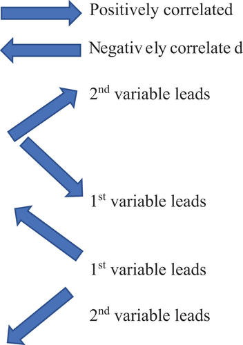
Figure 5 shows the directions of arrows and their meanings. When the two series are in-phases, it indicates that they move in a similar direction and anti-phase means that they move in the opposite direction. Arrows pointing to the right-down (South-East) or left-up (North-West) indicate that the first variable is leading, while arrows pointing to the right-up (North-East) or left-down (South-West) show that the second variable is leading.

Figure 5. Direction of arrows and their meaning.

From Figure 6, it is evident that the periods of turmoil caused by COVID-19’s first and second waves (around the second quarter and last quarter of 2020) are characterised by warmer colours. One should also note that the high correlations are found in the short- and medium-term horizon. This is indicative of financial contagion in its pure form; it is also worth noting that in periods of high correlation in short term, the arrows mainly point South-East, indicating a positive correlation between S&P500 and Bitcoin with S&P500 leading the causal effect. The presence of high correlation at lower scales (short-time horizon) indicates the presence of financial contagion, implying that the COVID-19 pandemic stimulated risky (irrational) behaviours among financial investors such as herd behaviour (Saiti et al., 2016). Another heating of the map is experienced in the medium-term horizon associated to 2 months or more (64 days) with arrow pointing North-East, indicating that the Bitcoin is leading S&P500. High correlation in the long-term horizon is indicative of co-movement due to fundamentals.

Figure 6. Wavelet coherence between S&P500 (developed equity market) and Bitcoin (cryptocurrency market). Directions of arrows and their meaning: → positively correlated, ←negatively correlated, ↗ 2nd variable (BTC) leads, ↘1^st variable (S&P500) leads, ↖1^st variable (S&P500) leads, and ↙2^nd variable (BTC) leads.

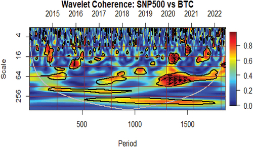
It is noteworthy that the stock markets lead the crypto market specifically in the short-term horizon. This means that the equity market react quicker to new information from crypto market. The implications thereof is that as far as the selected equity markets (advanced and emerging markets) are concerned, stability risks that might be caused by extreme price volatility emanating from cryptocurrency market can be ruled, for short-term to medium-term horizon, as spillovers occur in the reverse direction, that is from equity markets to crypto assets.

In order to analyse financial volatility spillovers between emerging markets and crypto market, a MODWT transformation was performed on a pair of return series of MSCI and Bitcoin. The MODWT used the Daubechies least asymmetric filter, with a wavelet filter length of 8 (LA) to examine financial contagion in the wake of the sub-prime crisis. The maximum level of MODTW is 8 (J₀ = 8). The wavelet analysis was performed with eight scales that span from two-day to one-and-a-half–year dyadic steps (2–4 days, 4–8 days, 8–16 days, 16–32 days, 32–64 days, 64–128 days, 128–256 days, and 256–512 days). Scales are presented on the horizontal axis and correlations on the vertical axis. To analyse statistical significance, 95% confidence intervals are used.

It can be seen in Figure 7 that the wavelet correlations between the MSCI and Bitcoin follow similar trend as the S&P 500, for instance the correlations tend to be constant around 0.2. However, there is a slight decrease on scale 6; after that the correlation increases again, reaching values close to unity at scale 8. This implies that discrepancies between the pairwise returns of the MSCI and Bitcoin do not dissipate for less than a year. In other words, for the more extended period, the correlation between MSCI and Bitcoin should not be ruled out. This can also be interpreted as perfect integration between MSCI and Bitcoin, in the sense that the MSCI returns can be determined by the overall performance of Bitcoin at horizons longer than a year.

Figure 7. Correlation of MSCI (emerging equity market) and Bitcoin (cryptocurrency market) at different time scales.

The study also examined cross-correlations between the MSCI and Bitcoin at all periods with the corresponding approximate confidence interval against lead time and lags for the different wavelet scales up to 33 days. The study thus calculates the cross-correlation of MSCI, and Bitcoin returns series first by lagging the Bitcoin series by 33-time units. The study then sequentially repeats the calculation of the cross-correlation for other time shifts (from 32-time units to the leads of 33-time units). If the curve is significant on the left, the first variable, i.e. MSCI, is leading. Conversely, if the curve is significant on the right side of the graph, the second variable, i.e. Bitcoin, is leading. It can be seen from Figure 8 that at the shortest scales, i.e. scales 1 to 2, there is no clear evidence of a lead-lag relationship, the cross-correlations. For scales 3 and 4, the cross-correlations around the time shift of π = 8 and π = −8 are significant and positive. It can also be seen that for scales 3 and 4, the graphs are slightly skewed to the left, indicating that the MSCI leads Bitcoin.

Figure 8. Cross-correlation between the return series of MSCI (emerging equity market) and Bitcoin (cryptocurrency market).

The scale 5 achieves the highest correlation at π = 19 and π = −19. And the graph is skewed to the right that the Bitcoin leads MSCI; for scales 6 and 7, there is no clear evidence of a lead-lag relationship. Finally, the contemporaneous time scale correlation between the series indicates the presence an anti-correlation relationship.

Figures 9 presents the estimated cross-wavelet coherence contour plots between the return series of MSCI and Bitcoin. The values for the 5% significance level represented by the curved line are obtained from Monte Carlo simulations. The name of the variable presented first is the first series (i.e. S&P 500), while the other one is the second series (i.e. Bitcoin). In wavelet coherence mapping, time is displayed on the horizontal axis—which is converted to time units (daily)—whereas the vertical axis shows the frequency (the lower the frequency, the higher the scale). One should note that the vertical axis, in our case of financial time series, can be interpreted as a period in days or as the investment horizon in days. Therefore, the higher the frequency, the lower is the investment period. The current study can therefore distinguish different scales in the frequency domain as short-term investment horizon (from beginning up to 16), medium-term investment horizon (from 32 days up to one year), and long-term investment horizon (beyond one year).

Figure 9. Wavelet coherence between MSCI (emerging market) and Bitcoin (cryptocurrency market). Directions of arrows and their meaning: → positively correlated, ← negatively correlated, ↗ 2nd variable(BTC) leads, ↘1^st variable(MSCI) leads, ↖ 1st variable (MSCI) leads, and ↙2^nd variable (BTC) leads.

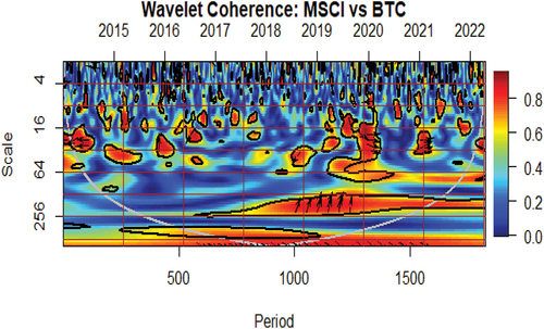
We can identify in Figure 9 a high correlation around the beginning of 2020 and mid-2020 and the time horizon associated to 2 weeks’ time scale; hence the conclusion that the co-movement is due to financial contagion. In period of high correlation, the arrows mainly point South-East, indicating a positive correlation between MSCI and Bitcoin with the MSCI leading. The presence of high correlation is also noticed in long-term horizon associated to 160 days with the arrows pointing North-East, indicating that the Bitcoin is leading MSCI. High correlation in short-term horizon during periods of financial upheaval is indicative of the presence of financial contagion between the cryptocurrency and equity markets, and it also suggests that cryptocurrency lost their safe-haven properties during periods of financial instability caused by COVID-19. The results confirm findings from previous studies by Buchwalter (2019) who found that contagion between crypto assets and equity markets is low during normal times but rises during periods of economic turmoil. There is high correlation between stock markets and crypto assets in the short to medium term. However, our findings in the long-run show non-existence of contagion between crypto assets and stock markets. This is in line with studies such as Cobert et al. (2019), who find no contagion between crypto assets and other financial assets.

6. Conclusion

The present study examined the volatility of the pure (narrow) form of financial contagion between cryptocurrency and stock markets during the crisis caused by the COVID-19 pandemic. Two econometric models are used in the study; they are (1) the DCC GARCH model and (2) the wavelet analysis model. The DCC GARCH model was chosen due to its capability to capture time-varying conditional correlations and covariances

Using the DCC GARCH model, the study found the evidence of increasing conditional correlations between cryptocurrency and the equity markets in advanced and emerging economies. The increasing conditional correlation was mostly detected in periods of financial turmoil corresponding to the first quarter and the second quarter of 2020. The increase in conditional correlation during periods of financial upheaval (compared to a tranquil period) indicates the presence of the pure form of financial contagion.

The wavelet cross-correlation analysis showed the evidence of positive cross-correlation between the Bitcoin and the equity markets, and the cross-correlation was identified in both short- and medium-term horizons. In the short-term horizon, the equity markets lead the cryptocurrency market, while the cryptocurrency market leads equity markets in the medium term. The wavelet analysis results also revealed the presence of high correlation at the short- to medium-term horizon during the period of financial turmoil. High correlation during the period of financial turmoil indicates the existence of the pure form of financial contagion between Bitcoin and advance equity markets. The main finding of the study is that cross-market hedging strategies between cryptocurrency and the stock markets may be effective in times of normal market stability, but they are more likely to fail in times of financial or economic turmoil due to the increased interconnectedness between the two markets.

7. Policy implications

The current study found the evidence of financial contagion between the cryptocurrency and equity markets. In the short-term investment horizon, stock markets lead cryptocurrency markets, while in the medium-term horizon, the cryptocurrency market leads stock markets. The implications thereof are that, firstly, for optimal portfolio diversification and better management, investors should not rely on cryptocurrencies as an alternative asset (safe-haven) to provide shelter from turbulence in traditional markets. Secondly, the fact that in the medium-term horizon, the cryptocurrency market was found to lead equity markets implies that policymakers, investors, and regulatory authorities should monitor closely the movement in the cryptocurrencies markets—for the medium-term investment horizon—and design appropriate regulatory policies to mitigate systemic risks emanating from cryptocurrencies.

Disclosure statement

No potential conflict of interest was reported by the authors.

Additional information

Notes on contributors

Olivier Niyitegeka

Olivier Niyitegeka is a Curriculum Practitioner at Regenesys Business School. His research interests include international economics, behavioural finance, financial risk management, time series, analysis of macroeconomic variables, and development economics.

Sheunesu Zhou

Sheunesu Zhou is an economist based at the University of Zhou. His research interests include Financial Economics, Macroeconomics, and Economic Development.

Notes

1. For example, if compared to the pre-pandemic year, the correlation between Bitcoin and S&P500 return has more than quadrupled (van de Schootbrugge, 2022).

2. Cryptocurrencies such as Bitcoin are often compared to gold due to their scarcity and decentralized nature, which makes them attractive to investors seeking protection against inflation and economic uncertainty. Their limited supply, like gold, adds to their perceived value, with only 21 million bitcoins available and no more to be produced once that number is reached.

3. This section relies heavily on Chittedi (2015).

4. The ARCH (AutoRegressive Conditional Heteroskedasticity) effect takes place when the variance of the current error term is related to the size of the previous period’s error term.

5. It should be drawn to the reader’s attention that while interpreting the result of wavelet phase-difference in the field of finance and economics, the leading role of one market over another market does not necessarily imply that there is a specific causality between the two. We should interpret with caution that the two markets, in fact, co-move with one market taking a leading role over another (Dewandaru et al., 2018).

6. Elon Musk, the CEO of Tesla and SpaceX, sent out a tweet on 12 May 2021 that said Tesla would no longer be accepting payments in Bitcoin owing to the high energy consumption of Bitcoin in the mining process. This decision sent cryptocurrencies into a downward spiral, and Bitcoin fell to nearly $30 000.

7. 18 May 2021, the People’s Bank of China (PBOC) announced that financial institutions in the country were prohibited from conducting any transactions involving cryptocurrencies, including Bitcoin.

References

- Ampountolas, A. (2022). Cryptocurrencies intraday high-frequency volatility spillover effects using univariate and multivariate GARCH models. International Journal of Financial Studies, 10(3), 51. https://doi.org/10.3390/ijfs10030051
- Begušić, S., Kostanjčar, Z., Stanley, H. E., & Podobnik, B. (2018). Scaling properties of extreme price fluctuations in Bitcoin markets. Physica A: Statistical Mechanics and Its Applications, 510, 400–21. https://doi.org/10.1016/j.physa.2018.06.131
- Bhosale, J., & Mavale, S. (2018). Volatility of select crypto-currencies: A comparison of Bitcoin, Ethereum and Litecoin. Annual Research Journal of SCMS, Pune, (6), 132–141. https://www.scmspune.ac.in/journal/pdf/current/Paper%2010%20-%20Jaysing%20Bhosale.pdf
- Biju, A. V., Mathew, A. M., Nithi Krishna, P. P., & Akhil, M. P. (2022). Is the future of Bitcoin safe? A triangulation approach in the reality of BTC market through a sentiments analysis. Digital Finance, (4), 275–290. https://link.springer.com/article/10.1007/s42521-022-00052-y
- Buchwalter, B. (June 4, 2019). Contagious Volatility. Proceedings of Paris December 2019 Finance Meeting EUROFIDAI - ESSEC. https://doi.org/10.2139/ssrn.3478511
- Catania, L., & Grassi, S. (2017). Modelling Crypto-currencies Financial Time-series. Tor Vergata University.
- Chinzara, Z., & Aziakpon, M. J. Dynamic returns linkages and volatility transmission between South African and world major stock markets. (2009). Journal of Studies in Economics and Econometrics, 33(3), 69–94. 33(3): 69-94. Studies in Economics and Econometrics. https://doi.org/10.1080/10800379.2009.12106473
- Corbet, S. Lucey, B., Yarovaya, L., Urquhart, A. (2019). Cryptocurrencies as a financial asset: A systematic analysis. International Review of Financial Analysis, 62, 182–189. https://centaur.reading.ac.uk/79186/1/CorbetLuceyUrquhartYarovaya2018.pdf
- Dajčman, S. (2013). Co-exceedances in Eurozone sovereign bond markets: Was there a contagion during the global financial crisis and the Eurozone debt crisis. Acta Polytechnica Hungarica, 10(3), 135–152. http://www.epa.hu/02400/02461/00041/pdf/EPA02461_acta_polytechnica_hungarica_2013_03_135-152.pdf
- Dewandaru, G., Masih, R., & Masih, M. (2018). Unraveling the financial contagion in European stock markets during financial crises: Multi-timescale analysis. Emerging Markets Finance and Trade, 54(4), 859–880. https://doi.org/10.1080/1540496X.2016.1266614
- Diebold, F. X., & Yilmaz, K. (2012). Better to give than to receive: Predictive directional measurement of volatility spillovers. International Journal of Forecasting, 28(1), 57–66. https://doi.org/10.1016/j.ijforecast.2011.02.006
- Dutta, A., Das, D., Jana, R. K., & Vo, X. V. (2020). COVID-19 and oil market crash: Revisiting the safe haven property of gold and Bitcoin. Resources Policy, 69, 101816. https://doi.org/10.1016/j.resourpol.2020.101816
- Engle, R. (2002). Dynamic conditional correlation: A simple class of multivariate generalized autoregressive conditional heteroskedasticity models. Journal of Business & Economic Statistics, 20(3), 339–350. https://doi.org/10.1198/073500102288618487
- Fakhfekh, M., & Jeribi, A. (2020). Volatility dynamics of crypto-currencies’ returns: Evidence from asymmetric and long memory GARCH models. Research in International Business and Finance, 51, 101075. https://doi.org/10.1016/j.ribaf.2019.101075
- Gençay, R., Selçuk, F., & Whitcher, B. (2003). Systematic risk and timescales. Quantitative Finance, 3(2), 108. http://repository.bilkent.edu.tr/bitstream/handle/11693/24504/bilkent-research-paper.pdf?sequence=1
- Gupta, H., & Chaudhary, R. (2022). An empirical study of volatility in cryptocurrency market. Journal of Risk and Financial Management, 15(11), 513. https://doi.org/10.3390/jrfm15110513
- Hashim, K. K., & Masih, A. (2015). Stock Market Volatility and Exchange Rates: MGARCH-DCC and wavelet approaches. University Library of Munich.
- Hung, N. T. (2022). Asymmetric connectedness among S&P 500, crude oil, gold and Bitcoin. Managerial Finance, 48(4), 587–610. https://doi.org/10.1108/MF-08-2021-0355
- Huynh, T. L. D., Ahmed, R., Nasir, M. A., Shahbaz, M., & Huynh, N. Q. A. (2021). The nexus between black and digital gold: Evidence from US markets. Annals of Operations Research, 1–26. https://doi.org/10.1007/s10479-021-04192-z
- In, F., & Kim, S. (2013). An Introduction to Wavelet Theory in Finance: A Wavelet Multiscale Approach. World Scientific.
- Iyer, T. (2022). Cryptic Connections: Spillovers between Crypto and Equity Markets. International Monetary Fund.
- Karim, B. A., Abdul-Rahman, A., HWANG, J. Y. T., & Kadri, N. (2021). Portfolio diversification benefits of cryptocurrencies and ASEAN-5 stock markets. The Journal of Asian Finance, Economics and Business, 8(6), 567–577.
- Khan, M., & Khan, M. (2021). Cryptomarket volatility in times of COVID-19 pandemic: application of GARCH models. Economic Research Guardian, 11(2), 2–13.
- Kumar, A. S., & Anandarao, S. (2019). Volatility spillover in crypto-currency markets: Some evidences from GARCH and wavelet analysis. Physica A: Statistical Mechanics and Its Applications, 524, 448–458. https://doi.org/10.1016/j.physa.2019.04.154
- Kumar, A., Iqbal, N., Mitra, S. K., Kristoufek, L., & Bouri, E. (2022). Connectedness among major cryptocurrencies in standard times and during the COVID-19 outbreak. Journal of International Financial Markets, Institutions and Money, 77, 101523. https://doi.org/10.1016/j.intfin.2022.101523
- Li, Z., Dong, H., Floros, C., Charemis, A., & Failler, P. (2022). Re-examining Bitcoin volatility: A CAViaR-based approach. Emerging Markets Finance and Trade, 58(5), 1320–1338. https://doi.org/10.1080/1540496X.2021.1873127
- Lucey, B. M., Vigne, S. A., Yarovaya, L., & Wang, Y. (2022). The cryptocurrency uncertainty index. Finance Research Letters, 45, 102147. https://doi.org/10.1016/j.frl.2021.102147
- Murty, S., Victor, V., & Fekete-Farkas, M. (2022). Is Bitcoin a safe haven for Indian investors? A GARCH volatility analysis. Journal of Risk and Financial Management, 15(7), 317. https://doi.org/10.3390/jrfm15070317
- Naimy, V., Haddad, O., Fernández-Avilés, G., El Khoury, R., & Trinidad Segovia, J. E. (2021). The predictive capacity of GARCH-type models in measuring the volatility of crypto and world currencies. PloS One, 16(1), e0245904. https://doi.org/10.1371/journal.pone.0245904
- Othman, A. H. A., Alhabshi, S. M., & Haron, R. (2019). The effect of symmetric and asymmetric information on volatility structure of crypto-currency markets: A case study of Bitcoin currency. Journal of Financial Economic Policy, 11(3), 432–450. https://doi.org/10.1108/JFEP-10-2018-0147
- Özdemir, O. (2022). Cue the volatility spillover in the cryptocurrency markets during the COVID-19 pandemic: Evidence from DCC-GARCH and wavelet analysis. Financial Innovation, 8(1), 1–38. https://doi.org/10.1186/s40854-021-00319-0
- Percival, D. P. (1995). On estimation of the wavelet variance. Biometrika, 83(2), 619–631. https://doi.org/10.1093/biomet/82.3.619
- Percival, D. B., & Walden, A. T. (2000). In Wavelet methods for time series analysis (Vol. 4). Cambridge university press. https://web.archive.org/web/20170808215030id_/http://tocs.ulb.tu-darmstadt.de/179403451.pdf
- Percival, D. B., & Walden, A. T. (2006). Wavelet Methods for Time Series Analysis (Vol. 4). Cambridge University Press.
- Ranta, M. (2010). Wavelet Multiresolution Analysis of Financial Time Series. Vaasan yliopisto.
- Saiti, B., Bacha, O. I., & Masih, M. (2016). Testing the conventional and Islamic financial market contagion: Evidence from wavelet analysis. Emerging Markets Finance and Trade, 52(8), 1832–1849. https://doi.org/10.1080/1540496X.2015.1087784
- Saleh, F. (2019). Volatility and Welfare in a Crypto Economy. McGill University. https://www.tse-fr.eu/sites/default/files/TSE/documents/sem2018/finance/saleh.pdf
- Salisu, A. A., & Ogbonna, A. E. (2021). The return volatility of cryptocurrencies during the COVID-19 pandemic: Assessing the news effect. Global Finance Journal, 54, 100641. https://doi.org/10.1016/j.gfj.2021.100641
- Shahzad, S. J. H., Bouri, E., Rehman, M. U., & Roubaud, D. (2022). The hedge asset for BRICS stock markets: Bitcoin, gold or VIX. The World Economy, 45(1), 292–316. https://doi.org/10.1111/twec.13138
- Srnic, B. S. (2014). Impact of Economic Crisis Announcements on BRIC Market Volatility. Faculty of Social sciences, Charles University in Prague.
- van de Schootbrugge, S., 2022. How crypto affects the global stock market and equities. [online] macro hive. Available at: https://macrohive.com/deep-dives/how-crypto-impacts-global-equity-prices/ [Retrieved July 20, 2022].
- Xu, F., Bouri, E., & Cepni, O. (2022). Blockchain and crypto-exposed US companies and major cryptocurrencies: The role of jumps and co-jumps. Finance Research Letters, 50, 103201. https://doi.org/10.1016/j.frl.2022.103201
- Yousaf, I., Ali, S., Bouri, E., & Saeed, T. (2022). Information transmission and hedging effectiveness for the pairs crude oil-gold and crude oil-Bitcoin during the COVID-19 outbreak. Economic Research-Ekonomska Istraživanja, 35(1), 1913–1934. https://doi.org/10.1080/1331677X.2021.1927787