On regime-switching European option pricing

Abstract

The concern of this article is to derive a regime switching model that can be utilized to price European call options for a financial market that exhibits structural changes with time. The model is formulated based on the fact that the underlying asset process is described by a geometric Brownian motion that is modulated by a continuous-time Markov chain with two regimes. Moreover, by an application of the change of measure technique, an option price is derived under the risk neutral valuation and the model parameter estimates is performed by use of the maximum likelihood estimation. The model implementation is carried out by utilizing the Russell 2000 and Facebook in dices data sets. The model results are compared with that of the Black-Scholes model in order to establish the model with better results in terms of predicting the European call option prices. In general, the data sets have common characteristics of financial time series across the regimes and the volatility process spends longer time in regime 2 than it stays in regime 1. The predicted call option prices from both models are more or less similar across the market indices; however, the results of the Black-Scholes model are a bit closer to the market prices than that of the regime-switching model across the two markets. Therefore, the Black-Scholes model slightly gives better results for the Russell 2000 and Facebook indices data sets as compared with the RS model.

Keywords:

• Volatility
• stock returns
• Black-Scholes model
• regimes
• regime-switching model

Public Interest Statement

In view of the existing literature, there is limited evidence that regime-switching (RS) model performs better than the famous Black-Scholes model in terms of pricing European options. This study develops a RS model for pricing European options in the event that the underlying asset dynamics depend on market regimes. The model developed here, when implemented to compute the European options, can help investors in making decision on when to trade their assets in order to get positive returns.

1 Introduction

The current literature portrays the Black-Scholes formula as the most broadly utilized in option pricing. The model utilizes the Geometric Brownian motion in capturing the dynamics of the underlying asset and it is assumed that the two model parameters, that is, the expected rate of return and the volatility, are deterministic, see Yao et al. (2006). Furthermore, the model assumes that volatility is steady until the lapse date, however, volatility is known to fluctuate with time, that is, it is a well-known fact that the financial market is stochastic in nature, see Mitsui and Satoyoshi (2010). It is thus evident that the Black-Scholes model cannot capture both the stochastic variability of the market dynamics and the volatility smile (the implied volatility of the underlying security). To address these shortfalls of the B-S model in modeling the financial market dynamics, the RS model of Hamilton (1989) has received an extensive application in the context of pricing derivatives. This model allows its parameters to flexibly change over time in accordance with the underlying state process that follow a Markov chain. Furthermore, the model has the ability to reproduce the common stylized facts of financial time series such as fat tails, volatility clustering, among others. The models are also utilized to price and hedge long-dated options in addition to allowing recovery of volatility smiles exhibited by empirical option prices; see Yao et al. (2006) and Godin and Trottier (2021). In support of RS models exhibiting autonomous shifts in mean and variances, Bollen et al. (2000) and Hardy (2001), proposed a RS log-normal (RSLN) model in which log-returns follow a normal distribution with mean and variance that depend on regime variable. In a study to price both American and European options using RS model, Bollen (1998) utilizes lattice method and simulation, whereas Buffington and Elliott (2002) use risk-neutral pricing and derive a set of partial differential equations for option price.

The evaluation of European options has previously been done using Black and Scholes model. It is thus very important to formulate the variation in volatility and evaluate option prices. In an effort to understand the variation in volatility, we refer to Engle (1982) who proposed the ARCH model that formulates the volatility at each time as the linear function of the square of the past unexpected shock. Additionally, Bollerslev (1986), added the past volatility values to the explanatory variables and extended the GARCH (generalized ARCH) model. Empirical studies of options utilizing the GARCH model based on local risk neutrality, which was proposed by Duan (1995), have been conducted by Mitsui (2000), Duan and Zhang (2001), Bauwens and Lubrano (1998), Mitsui and Watanabe (2003). Incidentally, it is known that in RS model the persistence of shock on volatility is extremely high. However, Dieobold (1986) and Lamoureux and Lastrapes (1990) reported that such persistence is considered to be caused by the structural volatility change. It is therefore based on this fact, Hamilton and Susmel (1994) and Cai (1994) proposed the Markov-Switching ARCH (MS-ARCH) model using a state variable that follows the Markov process in the formulation of the ARCH model so as to take into account the structural change. Moreover, Gray (1996) proposed the Markov Switching GARCH model by taking into account the structural change in the GARCH model. Siu et al. (2004) proposed an option pricing model based on GARCH assumption for underlying assets in the context of dynamic version of Gerber-Shiu’s option-pricing model and utilized conditional Esscher Transforms to develop a martingale measure in the context of an incomplete market situation. Their results were consistent with that of Duan (1995) under the assumption of conditional normality for the stock innovation they their results are justified based on the dynamic framework of utility maximization problems as per the Gerber-Shiu’s option-pricing model. Barone-Adesi et al. (2008) in their research proposed option pricing method that was based on GARCH models with filtered historical innovations. Their model outperformed other GARCH pricing models and Black—Scholes models empirically for S&P 500 index options. The model did explain implied volatility smiles by the negative asymmetry of the filtered historical innovations. Empirical evidence and the extent of deterioration of the delta hedging in the presence of large volatility shock were revealed by the study.

Recently, studies on option pricing have been carried out, for instance, Biswas et al. (2018) used a RS stochastic model with a semi-Markov modulated square root mean reverting process to study European option pricing. Their study discovered the local risk-minimizing European-type vanilla options price and it was proven that the price function adequately meet a non-local degenerate parabolic PDE which is the general case of the Heston PDE model. A study by Deelstra et al. (2020) considers risk-neutral pricing of Vanilla, digital and down-and-out call options with the price of the underlying asset evolving according to the exponential of a Markov-modulated Brownian motion (MMBM) with two-sided phase-type jumps. Further, he documents that such options are closely related to the MMBM’s first passage properties which he analyzed by randomizing the time horizon using Erlang distribution. Moreover, Nasri et al. (2020) used a RS Copula model to option prices where serial independence of error terms for time series is presented which was subjected to several time series analysis. Moreover, Kirkby and Nguyen (2020) utilized duality and FFT-based density projection implementation to establish a novel and efficient transform approach for pricing Asian options for general asset dynamics, such as RS Levy processes and stochastic volatility models with jumps. In his research, Lin and He (2020) addressed the problem of pricing the European options using a RS finite moment log-stable model. Their model has the ability to represent the key features of asset returns as well as the impact of regime transition, and it is compatible with market findings. Furthermore, they state that option prices are driven by a coupled FPDE (Fractional Partial Differential Equation) system in their model. They note that their model can mimic option prices emanating from other existing models with particular parameter settings while also bringing into significance pricing differences relative to current models by changing parameter values, indicating that it has the potential to be used in practice. 2021) in his study reveals that Esscher transform approach for obtaining risk neutrality is famous in pricing options under RS models. However, this approach creates path-dependence in the dynamics of option price since under the physical measure; the underlying asset is integrated in a Markov process. To address the path-dependence they develop a novel and intuitive risk-neutral measures that integrates risk-aversion in regimes and consequently removing the path dependence side effects. Later on, the study of 2021) was complimented by Godin and Trottier (2019) who developed and utilized extended Girsanov principle which also removes the path-dependence effect. This model is easy to interpret in terms of consistence with hedging agents locally minimizing their risk-adjusted discounted squared hedging errors.

In view of the available literature, this study is certainly not the first one to deal with RS dynamics in financial markets or pricing options under RS. However, in terms of pricing European options there seem to be limited evidence that RS model gives better pricing results than the famous Black-Scholes models and thus further research in this area of European option pricing remains necessary. Therefore, the key objective of this study is to develop a RS model for pricing options when the underlying asset dynamics depend on the market regimes. The formulation of this model is based on a geometric Brownian motion that is governed by a continuous-time Markov chain with two states and applying a change of measure, an option price is derived under the risk-neutral valuation. Moreover, the model parameters are estimated using the maximum likelihood estimation method and finally, an implementation of the model is done by computing the European call option prices for some chosen stock market indices. The results of this model are compared with those of the Black-Scholes model with an aim to establish whether the RS model is a better and reliable model compared with the Black-Scholes model.

The organization of the rest of the paper is as follows. Section 1 outlines the derivation of the European option pricing RS model and estimation of parameters. Section 2 is the empirical analysis of the data to implement the model and lastly, section 3 concludes the paper.

2 Methodology

2.1 Regime switching market dynamics

Let $(X_t{)}_{t\ge 0}$ be a stochastic process on a discrete time set $\mathcal{T}=\{t,\dots ,T\}$ and $(\mathrm{\Omega },\mathcal{F},\mathbb{P})$ be a probability space, where $\mathbb{P}$ is a physical probability measure. Further let, $\xi (t)$ be Markov chain with $\mathcal{M}=\{1,\dots ,k\}$ states or regimes and transition probability $P_{i,j}$. We consider a risk-free asset, $d{S}_t^{\ast }=r{S}_t^{\ast }dt$ that is assumed to be continuously compounded in value at a constant risk-free rate, $r,$ (but not necessarily non-negative) over the trading time interval [t,T]. Taking $S_t^{\ast }=1$, the price of the asset at time $t$, is given by $S_t^{\ast }=e^{r\mathcal{T}}$. Consider a second market which is risky and whose price is defined as

(1) $S_T=S_{t}exp(\sum _{t=1}^T{X}_t),t\in \mathcal{T}$(1)

where $S_t$ is the initial price of the asset. The log-returns for the asset are given by

(2) $X_t={\mu }_{\xi (t)}+{\sigma }_{\xi (t)}{r}_t,\mathrm{w}\mathrm{h}\mathrm{e}\mathrm{r}\mathrm{e}{r}_t\sim i.i.dN(0,1).$(2)

The constants ${\mu }_{\xi (t)}\mathrm{a}\mathrm{n}\mathrm{d}{\sigma }_{\xi (t)}$ represents the mean and standard deviation of log-returns under each regime, $\xi (t)=1,2,\dots ,k$ and $r_t$ is a sequence of i.i.d random variables with zero mean and unit variance under measure $\mathbb{P}$ and independent from the Markov chain $\xi (t)$. The filtration ${\mathcal{F}}_t$ on the probability space $(\mathrm{\Omega },{\mathcal{F}}_t,\mathbb{P})$ contains all the information generated by all the underlying asset prices and realized regimes upto time $T$. However, the regimes are latent variables hence this filtration characterizes only a partial information to investors. Therefore, we assume that for $j\in \{1,\dots ,k\},$

(3) $\mathbb{P}[\xi (t+1)=j|{\mathcal{F}}_t]=P_{i,j}$(3)

where $P_{i,j}$ is the transition probability from state $i\to j$ of the Markov chain $\xi (t)$

2.2 Regime-switching model

We consider a risk-free asset and a risky asset as discussed earlier. These assets are tradable continuously over time in a finite time horizon $\tau =[t,T]$ where $T<\mathrm{\infty }$. In order to describe uncertainty, we consider a complete probability space $(\mathrm{\Omega },\mathcal{F},\mathbb{P})$ where $\mathbb{P}$ is a real world probability measure. According to Yao et al. (2006), in the RS world, one typically modulates the rate of return and the volatility by a finite-state Markov chain $\{\xi (t),t\ge 0\}$, which represents the market regime. Let $\{\xi (t),t\ge 0\}$ be continuous, finite-state, Markov process on $(\mathrm{\Omega },\mathcal{F},\mathbb{P})$ with state space $\mathcal{M}=\{1,2,\dots ,k\}$ and that $S_t$ is the stock price at time $t$ satisfying the stochastic differential equation defined by

(4) $\frac{d{S}_t}{S_t}={\mu }_{\xi (t)}dt+{\sigma }_{\xi (t)}d{W}_t,\xi (t)=\{1,2,\dots ,k\}$(4)

where $S_t>0$ is the initial price, $W_t$ is a standard Brownian motion independent of $\xi (t)$.

The parameters ${\mu }_{\xi (t)}$ and ${\sigma }_{\xi (t)}$ denote the expected rate of return on the asset and volatility of the asset price, respectively, and are assumed to be constant and distinct for each regime. In this way, $\xi (t)$ is regarded as a variable that chooses one of the states in $\mathcal{M}$ at time $t$ of the market. Equation (4)(4) $\frac{d{S}_t}{S_t}={\mu }_{\xi (t)}dt+{\sigma }_{\xi (t)}d{W}_t,\xi (t)=\{1,2,\dots ,k\}$(4) is solved using Itô lemma to give

(5) $S_T=S_t{e}^{({\mu }_{\xi (t)}-\frac{1}{2}{\sigma }_{\xi (t)}^2)\tau +{\sigma }_{\xi (t)}{W}_{\tau }},\mathrm{f}\mathrm{o}\mathrm{r}\xi (t)=\{1,2,\dots ,k\}$(5)

The stock price process in Equation (5)(5) $S_T=S_t{e}^{({\mu }_{\xi (t)}-\frac{1}{2}{\sigma }_{\xi (t)}^2)\tau +{\sigma }_{\xi (t)}{W}_{\tau }},\mathrm{f}\mathrm{o}\mathrm{r}\xi (t)=\{1,2,\dots ,k\}$(5) is assumed to exhibit regime switches. Let the price process undergo discrete shifts between regimes $\xi (t)$ and that it follows a first-order Markov chain, then the transition probability $P_{ij}$ from state $i$ at time $t+1$ to state $j$ at time $t$ is denoted by

(6) $P_{ij}=P\{\xi (t+1)=j|\xi (t)=i\}\mathrm{f}\mathrm{o}\mathrm{r}\mathrm{a}\mathrm{l}\mathrm{l}i,j=\{1,2,\dots ,k\}$(6)

where $0\le P_{ij}\le 1$ and ${\sum }_{j=1}^k{P}_{ij}=1$. The transition matrix $P_{ij}$ of the Markov chain is given by

$P_{ij}=\left[\begin{array}{cccc}{p}_{11}& p_{12}& \dots & p_{1k}\\ p_{21}& p_{22}& \dots & p_{2k}\\ .& .& \dots & .\\ .& .& \dots & .\\ .& .& \dots & .\\ p_{k1}& .& \dots & p_{kk}\end{array}\right]$

In particular, for a very small time interval $\delta >0$,

(7) $P(T<\delta )=1-e^{-{\lambda }_i\delta }=1-(1-{\lambda }_i\delta )={\lambda }_i\delta$(7)

That is, in a short interval of time $\delta >0$, the probability of leaving state $i$ is approximately ${\lambda }_i\delta$. This means, ${\lambda }_i$ is the transition rate out of state $i$ and can formally be expressed as

(8) ${\lambda }_i=\underset{\delta \to 0^{+}}{lim}\left[\frac{P(\xi (T)=j|\xi (t)=i}{\delta }\right]$(8)

Since $P_{ij}$ is the probability to move from state $i$ to state $j$, the quantity $g_{ij}={\lambda }_i{P}_{ij}$ is the transition rate from state $i$ to state $j$.

Definition 2.1 (Generator matrix)

Define a generator matrix, $\mathbb{G}$ for a continuous-time Markov chain. The $(i,j{)}^{th}$ element of the transition matrix is given by

(9) $g_{ij}=\left\{\begin{array}{c}{\lambda }_i{P}_{ij},i\ne j\\ -{\lambda }_i,i=j\end{array},Also{g}_{ii}=-\sum _{i\ne j}{g}_{ij}\right.$(9)

The generator matrix of the Markov chain is thus given by

$G=\left[\begin{array}{cccc}{\lambda }_{11}& {\lambda }_{12}& \dots & {\lambda }_{1k}\\ {\lambda }_{21}& {\lambda }_{22}& \dots & {\lambda }_{2k}\\ .& .& \dots & .\\ .& .& \dots & .\\ .& .& \dots & .\\ {\lambda }_{k1}& {\lambda }_{22}& \dots & {\lambda }_{kk}\end{array}\right]$

and, for each state, the elements of the generator matrix satisfy the equation ${\lambda }_{jj}+{\sum }_{i=1,i\ne j}^k{\lambda }_{ij}=0$. For small time interval $\delta >0$ and $i$ the probability to be in state $j$ at time $t+\delta$ given that the random variable was in state $i$ at time $t$ is given by

(10) $P(X(t+\delta )=j|X(t)=i)=g_{ij}.\delta +O(\delta )$(10)

where $O(\delta )$ is the probability from state $i$ to state $j$ in more than one step but ${lim}_{\delta \to 0}\left[\frac{O(\delta )}{\delta }\right]=0$.

The model developed here postulates that the regimes are unobservable and thus state transitions until maturity are considered. Denote by $\xi (t)$, the variable representing the regime in which the process was at time $t$. When the change in log price $X_t$ is in regime $j$, it is presumed to have been drawn from a normal distribution with mean, ${\mu }_j$ and variance, ${\sigma }_j^2$. Hence, the probability density function of $X_t$ conditional on $\xi (t)$ taking on the value $j$ is given by

(11) $f(X_t|\xi (t)=j;\theta )=\frac{1}{{\sigma }_j\sqrt{2\pi }}exp\left\{-\frac{{(X_t-{\mu }_j)}^2}{2{\sigma }_j^2}\right\}$(11)

for $j=\{1,2,\dots ,k\}$ and $\theta$ is a vector of parameters ${\mu }_j,{\sigma }_j\mathrm{f}\mathrm{o}\mathrm{r}j=1,2,\dots ,k$, that is, $\theta =\{{\mu }_j,{\sigma }_j{\}}^{\prime }$ Furthermore, it is presumed that the unobserved regime $\xi (t)$ have been generated by a probability distribution for which the conditional probability that $\xi (t)=j$ given the information up to time $t$ is denoted by ${\pi }_j$, that is

(12) $P\{\xi (t)=j|{\mathcal{F}}_t;\theta \}={\pi }_j\mathrm{f}\mathrm{o}\mathrm{r}j=\{1,2,\dots ,k\}$(12)

Thus, the vector $\theta$ also includes ${\pi }_j\mathrm{f}\mathrm{o}\mathrm{r}j=1,2,\dots ,k$, that is, $\theta =\{{\mu }_j,{\sigma }_j,{\pi }_j{\}}^{\prime }$. Next is to find the probability of the joint event that $\xi (t)=j$ and $X_t$ falls within some time interval [t,T]. This is determined by integrating

(13) $p(X_t,\xi (t)=j;\theta )=f(X_t|\xi (t)=j;\theta )P(\xi (t)=j|{\mathcal{F}}_t;\theta )$(13)

over all values of $X_t$ between $t$ and $t$. The Equation (13)(13) $p(X_t,\xi (t)=j;\theta )=f(X_t|\xi (t)=j;\theta )P(\xi (t)=j|{\mathcal{F}}_t;\theta )$(13) is the joint probability density function of $\xi (t)$ and $X_t$ and by utilizing Equations (11) and (12), it is expressed as

(14) $p(X_t,\xi (t)=j;\theta )=\frac{{\pi }_j}{{\sigma }_j\sqrt{2\pi }}exp\left\{-\frac{{(X_t-{\mu }_j)}^2}{2{\sigma }_j^2}\right\}\mathrm{f}\mathrm{o}\mathrm{r}j=\{1,2,\dots ,k\}$(14)

The unconditional probability density function of $X_t$ is determined by summing Equation (14)(14) $p(X_t,\xi (t)=j;\theta )=\frac{{\pi }_j}{{\sigma }_j\sqrt{2\pi }}exp\left\{-\frac{{(X_t-{\mu }_j)}^2}{2{\sigma }_j^2}\right\}\mathrm{f}\mathrm{o}\mathrm{r}j=\{1,2,\dots ,k\}$(14) over all values for $j$:

(15) $\begin{array}{cc}f(X_t;\theta )& =\sum _{j=1}^{k}p(X_t,\xi (t)=j;\theta )\\ \hspace{0.17em}& =\frac{{\pi }_1}{\sqrt{2\pi }{\sigma }_1}exp\left\{-\frac{{(X_t-{\mu }_1)}^2}{2{\sigma }_1^2}\right\}+\dots +\frac{{\pi }_j}{\sqrt{2\pi }{\sigma }_j}exp\left\{-\frac{{(X_t-{\mu }_j)}^2}{2{\sigma }_j^2}\right\}\end{array}$(15)

Again, based on the definition of conditional probability,

(16) $P[\xi (t)=j|X_t;\theta ]=\frac{p(X_t,\xi (t)=j;\theta )}{f(X_t;\theta )}=\frac{{\pi }_{j}f(X_t|\xi (t)=j;\theta )}{f(X_t;\theta )}$(16)

Note that the magnitude in Equation (16)(16) $P[\xi (t)=j|X_t;\theta ]=\frac{p(X_t,\xi (t)=j;\theta )}{f(X_t;\theta )}=\frac{{\pi }_{j}f(X_t|\xi (t)=j;\theta )}{f(X_t;\theta )}$(16) for each observation $X_t$ in the sample can be calculated if the knowledge of the parameters $\theta$ is known by use of Equations (11(11) $f(X_t|\xi (t)=j;\theta )=\frac{1}{{\sigma }_j\sqrt{2\pi }}exp\left\{-\frac{{(X_t-{\mu }_j)}^2}{2{\sigma }_j^2}\right\}$(11) -14(14) $p(X_t,\xi (t)=j;\theta )=\frac{{\pi }_j}{{\sigma }_j\sqrt{2\pi }}exp\left\{-\frac{{(X_t-{\mu }_j)}^2}{2{\sigma }_j^2}\right\}\mathrm{f}\mathrm{o}\mathrm{r}j=\{1,2,\dots ,k\}$(14) ). Equation (16)(16) $P[\xi (t)=j|X_t;\theta ]=\frac{p(X_t,\xi (t)=j;\theta )}{f(X_t;\theta )}=\frac{{\pi }_{j}f(X_t|\xi (t)=j;\theta )}{f(X_t;\theta )}$(16) represent probability, given the observed data, that the unobserved regime responsible for observation $t$ was regime $j$. The probability of $\xi (t)=j$ given the information ${\mathcal{F}}_t$ up to time $t$, that is, $P[\xi (t)=j|{\mathcal{F}}_t]$ can be calculated by first calculating

(17) $P[\xi (t-1)=i|{\mathcal{F}}_{t-1}]\mathrm{f}\mathrm{r}\mathrm{o}\mathrm{m}P[\xi (t)=j|{\mathcal{F}}_{t-1}]$(17)

with the following equation

(18) $\begin{array}{cc}P[\xi (t)=j|{\mathcal{F}}_{t-1}]& =\sum _{j=1}^{k}P[\xi (t)=j,\xi (t-1)=i|{\mathcal{F}}_{t-1}]\\ \hspace{0.17em}& =\sum _{j=1}^{k}P[\xi (t)=j|\xi (t-1)=i]P[\xi (t-1)=i|{\mathcal{F}}_{t-1}]\end{array}$(18)

where $P[\xi (t)=j|\xi (t-1)=i]$ is the transition probability as earlier defined. Next, adding the data $X_t$ at the time $t$ leads to the equation

(19) $\begin{array}{cc}P[\xi (t)=j|{\mathcal{F}}_{t-1},X_t]& =\frac{f(\xi (t)=j,X_t|{\mathcal{F}}_{t-1})}{f(X_t|{\mathcal{F}}_{t-1})}\\ \hspace{0.17em}& =\frac{f(X_t|\xi (t)=j,{\mathcal{F}}_{t-1})P[\xi (t)=j|{\mathcal{F}}_{t-1}]}{{\sum }_{j=1}^{2}f(X_t|\xi (t)=j,{\mathcal{F}}_{t-1})P[\xi (t)=j|{\mathcal{F}}_{t-1}]}\end{array}$(19)

Note that the probability, $P[\xi (t)=j|{\mathcal{F}}_{t-1}]$ for $t=1,2,\dots ,T$ can be obtained by repeating the calculations of Equations (18(18) $\begin{array}{cc}P[\xi (t)=j|{\mathcal{F}}_{t-1}]& =\sum _{j=1}^{k}P[\xi (t)=j,\xi (t-1)=i|{\mathcal{F}}_{t-1}]\\ \hspace{0.17em}& =\sum _{j=1}^{k}P[\xi (t)=j|\xi (t-1)=i]P[\xi (t-1)=i|{\mathcal{F}}_{t-1}]\end{array}$(18) ,19(19) $\begin{array}{cc}P[\xi (t)=j|{\mathcal{F}}_{t-1},X_t]& =\frac{f(\xi (t)=j,X_t|{\mathcal{F}}_{t-1})}{f(X_t|{\mathcal{F}}_{t-1})}\\ \hspace{0.17em}& =\frac{f(X_t|\xi (t)=j,{\mathcal{F}}_{t-1})P[\xi (t)=j|{\mathcal{F}}_{t-1}]}{{\sum }_{j=1}^{2}f(X_t|\xi (t)=j,{\mathcal{F}}_{t-1})P[\xi (t)=j|{\mathcal{F}}_{t-1}]}\end{array}$(19) ), and the results substituted into Equation (14)(14) $p(X_t,\xi (t)=j;\theta )=\frac{{\pi }_j}{{\sigma }_j\sqrt{2\pi }}exp\left\{-\frac{{(X_t-{\mu }_j)}^2}{2{\sigma }_j^2}\right\}\mathrm{f}\mathrm{o}\mathrm{r}j=\{1,2,\dots ,k\}$(14) .

In order to price options, it is key to derive a pricing model that produces no arbitrage (a situation where investors can make a guaranteed profit without incurring risk). To avoid arbitrage, the options are priced under risk neutral measure or martingale measure. Under the physical probability measure $\mathbb{P}$, we wish to have $e^{-{\int }_t^{T}rds}{S}_t$ to be a martingale. Here, $r$ is the risk-free interest rate and it is assumed to be constant across the regimes. Since $S_t$ denotes the price of a stock at time $t$ which satisfies Equation (4)(4) $\frac{d{S}_t}{S_t}={\mu }_{\xi (t)}dt+{\sigma }_{\xi (t)}d{W}_t,\xi (t)=\{1,2,\dots ,k\}$(4) , we assume that $\xi (t),\mathrm{a}\mathrm{n}\mathrm{d}{W}_t$ are mutually independent; and ${\sigma }_{\xi (t)}^2>0$, for all $\xi (t)\in \mathcal{M}$. Suppose that $\{\xi (u),W(u):0\le u\le t\}$ denote the sigma field generated by ${\mathcal{F}}_t$. We note that all(local) martingales concerned are with respect to the filtration. It is clear that $\{W_t\}$ and $\{W_t^2-t\}$, are both martingales. Define an equivalent measure $\mathbb{Q}$ under which the discounted stock process is a martingale. Let the risk-free rate be denoted by $r>0$. Then for $0\le t\le T$, let

(20) $Z_t=exp\left({\int }_t^T{\beta }_{s}d{W}_s-\frac{1}{2}{\int }_t^T{\beta }_s^{2}ds\right)$(20)

where ${\beta }_s=\frac{\mu (\xi (u))-r}{\sigma (\xi (u))}$. By Girsanov’s theorem, the process

(21) ${\tilde{W}}_t=W_t-{\int }_t^T{\beta }_{s}ds\Rightarrow d{\tilde{W}}_t=d{W}_t-{\beta }_{t}dt$(21)

is a $\mathbb{Q}$-Brownian motion. Moreover, applying Ito’s rule results to $\frac{d{Z}_t}{Z_t}={\beta }_{t}d{W}_t$ where $Z_t$ is a local martingale, with $\mathbb{E}[Z_t]=1,0\le t\le T$. An equivalent measure $\mathbb{Q}$ is defined via the Radon-Nikodym derivative, $\frac{d\mathbb{Q}}{d\mathbb{P}}=Z_T$. Combining Equations (4) and(21) gives

(22) $\frac{d{S}_t}{S_t}=rdt+{\sigma }_{\xi (t)}d{\tilde{W}}_t\mathrm{w}\mathrm{h}\mathrm{o}\mathrm{s}\mathrm{e}\mathrm{s}\mathrm{o}\mathrm{l}\mathrm{u}\mathrm{t}\mathrm{i}\mathrm{o}\mathrm{n}\mathrm{i}\mathrm{s}{S}_T=S_{t}exp\left[(r-\frac{1}{2}{\sigma }_{\xi (t)}^2)\tau +{\sigma }_{\xi (t)}{\tilde{W}}_{\tau }\right]$(22)

This model has two types of random sources, $W_t\mathrm{a}\mathrm{n}\mathrm{d}\xi (t)$ and the inclusion of $\xi (t)$ makes the underlying market incomplete.

Let $\mathcal{R}$ denote the total time spent in regime $\xi (t)=j\mathrm{f}\mathrm{o}\mathrm{r}j=1,2,\dots ,k$ in the interval $[t,T]$ in $n$ trials, given that at time $t$, the state is $k$. Denote the probability $Pr(\mathcal{R}={\alpha }_j)$ by $p$ for $j=1,2,\dots ,k-1$. For simplicity, we restrict ourselves to two regimes, i.e, $k=2$, hence the transition matrix, discussed earlier, reduces to

$P_{ij}=\left[\begin{array}{cc}{p}_{11}& p_{12}\\ p_{21}& p_{22}\end{array}\right]$

The fraction of times spent by the Markov chain in each regime, as the numbers of transitions $n$ become large, can be calculated using a time-average (invariant) distribution of the Markov chain, that is $\beta P=\beta$, where $P$ is the transition matrix and $\beta$ is the average fraction of the time spent in state $\xi (t)=j$ over $n$ steps as n approaches infinity. Let $\beta =[{\beta }_1{\beta }_2]$, then

(23) $[\beta P]=[{\beta }_1{\beta }_2]\left[\begin{array}{cc}{p}_{11}& p_{12}\\ p_{21}& p_{22}\end{array}\right]=[{\beta }_1{\beta }_2]$(23)

This results into two equations as ${\beta }_1{P}_{11}+{\beta }_2{P}_{21}=\beta 1\mathrm{a}\mathrm{n}\mathrm{d}{\beta }_1{P}_{12}+{\beta }_2{P}_{22}={\beta }_2$ both of which simplify to ${\beta }_1{P}_{12}={\beta }_2{P}_{21}(\mathrm{s}\mathrm{i}\mathrm{n}\mathrm{c}\mathrm{e}{P}_{11}+P_{12}=1\mathrm{a}\mathrm{n}\mathrm{d}{P}_{21}+P_{22}=1)$. Again, since $\beta$ is a valid probability distribution, ${\beta }_1+{\beta }_2=1$ and solving we get

(24) ${\beta }_1=\frac{P_{21}}{P_{12}+P_{21}}\mathrm{a}\mathrm{n}\mathrm{d}{\beta }_2=\frac{P_{12}}{P_{12}+P_{21}}$(24)

Since, $\tau =T-t$ is the trading period, the total time spent in regimes 1 and 2 can now be calculated as $\mathcal{R}={\beta }_1\tau \mathrm{a}\mathrm{n}\mathrm{d}\tau -\mathcal{R}=\tau -{\beta }_1\tau$, respectively. In view of the research by Duan et al. (2002) and Hardy (2001) the distribution of log returns, $X_t=log(\frac{S_T}{S_t})$, conditional on the total time spent in regime $\xi (t)=j,\mathrm{f}\mathrm{o}\mathrm{r}j=1,2$, $k$ can be developed such that there exist a normal density function with mean ${\mu }^{\ast }$ and variance ${{\sigma }^{\ast }}^2$, that is,

(25) $X_t|\mathcal{R}\sim N({\mu }^{\ast },{{\sigma }^{\ast }}^2)$(25)

where ${\mu }^{\ast }=\frac{\mathcal{R}}{\tau }{\mu }_1+(\frac{\tau -\mathcal{R}}{\tau }){\mu }_2\mathrm{a}\mathrm{n}\mathrm{d}\sigma {\ast }^2=\frac{\mathcal{R}}{\tau }{\sigma }_1^2+(\frac{\tau -\mathcal{R}}{\tau }){\sigma }_2^2$. Since $p$ is the probability function for $\mathcal{R}$,

(26) $\begin{array}{cc}{F}_{X_t}=Pr[X_t\le x]& =\sum _{j=1}^{k-1}Pr[X_t|\mathcal{R}={\alpha }_j]p\\ \hspace{0.17em}& =\sum _{j=1}^{k-1}\varphi \left(\frac{x-\mu \ast }{\sigma \ast }\right)p\end{array}$(26)

where $\varphi ()$ is the standard normal probability distribution function. This implies that the probability density function for $X_t$ is

(27) $f_{X_t}=\sum _{j=1}^{k-1}\varphi (\frac{x-\mu \ast }{\sigma \ast })p$(27)

where $\varphi ()$ is the standard normal density function.

Now, define $C(K,T)$, the European call option (under RS world) with strike price $K$ that matures after time $T$, and is valued at $S_t$ at an initial time $t$. Since in a RS market, the parameter ${\sigma }^2$ switches regimes, we can define a parameter $\sigma {\ast }^2$ conditional on knowing $\mathcal{R}$, the total time spent in regime $\xi (t)=j\mathrm{f}\mathrm{o}\mathrm{r}j=1,2$. This implies that, the asset price $S_t|\mathcal{R}$ has a log normal distribution with parameters that depend on $\mathcal{R}$, that is, the parameters are $\mu \ast \mathrm{a}\mathrm{n}\mathrm{d}\sigma {\ast }^2$ as defined earlier. Now, to derive a RS option pricing model, the Black-Scholes formula is considered, where the parameter ${\sigma }^2$ is replaced with $\sigma {\ast }^2$ to give the desired model as below;

(28) $C(K,T)={\mathbb{E}}^{\mathbb{Q}}[max(X_T-K)|\mathcal{R}]=S_t\varphi (d_1)-e^{-r\tau }K\varphi (d_2)\mathrm{w}\mathrm{h}\mathrm{e}\mathrm{r}\mathrm{e}$(28)

$d_1=\frac{ln(\frac{S_t}{K})+r\tau +\frac{1}{2}[\mathcal{R}{\sigma }_1^2+(\tau -\mathcal{R}){\sigma }_2^2]}{\sqrt{\mathcal{R}{\sigma }_1^2+(\tau -\mathcal{R}){\sigma }_2^2}}$

$d_2=d_1-\sqrt{\mathcal{R}{\sigma }_1^2+(\tau -\mathcal{R}){\sigma }_2^2}$

2.2.1 Model parameter estimates

Equation (15)(15) $\begin{array}{cc}f(X_t;\theta )& =\sum _{j=1}^{k}p(X_t,\xi (t)=j;\theta )\\ \hspace{0.17em}& =\frac{{\pi }_1}{\sqrt{2\pi }{\sigma }_1}exp\left\{-\frac{{(X_t-{\mu }_1)}^2}{2{\sigma }_1^2}\right\}+\dots +\frac{{\pi }_j}{\sqrt{2\pi }{\sigma }_j}exp\left\{-\frac{{(X_t-{\mu }_j)}^2}{2{\sigma }_j^2}\right\}\end{array}$(15) best describes the actually observed data $X_t$ since the regime $\xi (t)$ is unobserved. If the regime variable $\xi (t)$ is i.i.d across different dates, $t$, then the log likelihood for the observed data can be calculated from Equation (15)(15) $\begin{array}{cc}f(X_t;\theta )& =\sum _{j=1}^{k}p(X_t,\xi (t)=j;\theta )\\ \hspace{0.17em}& =\frac{{\pi }_1}{\sqrt{2\pi }{\sigma }_1}exp\left\{-\frac{{(X_t-{\mu }_1)}^2}{2{\sigma }_1^2}\right\}+\dots +\frac{{\pi }_j}{\sqrt{2\pi }{\sigma }_j}exp\left\{-\frac{{(X_t-{\mu }_j)}^2}{2{\sigma }_j^2}\right\}\end{array}$(15) as

(29) $L(\theta )=\sum _{t=1}^{T}logf(X_t;\theta )$(29)

The maximum likelihood of $\theta$ is obtained by maximizing Equation (29)(29) $L(\theta )=\sum _{t=1}^{T}logf(X_t;\theta )$(29) subject to the constraints that ${\pi }_1+{\pi }_2=1$ and ${\pi }_j\ge 0$ for $j=1,2$. To obtain the maximum likelihood estimates(MLEs) of Equation (29)(29) $L(\theta )=\sum _{t=1}^{T}logf(X_t;\theta )$(29) we form the Lagrangian

(30) $J(\theta )=L(\theta )+\lambda (1-{\pi }_1-{\pi }_2)$(30)

and set the derivative w.r.t $\theta$ equal to zero. From Equation (29)(29) $L(\theta )=\sum _{t=1}^{T}logf(X_t;\theta )$(29) , the derivative of the log likelihood is given by

(31) $\frac{\mathrm{\partial }L(\theta )}{\mathrm{\partial }\theta }=\sum _{t=1}^T\frac{1}{f(X_t;\theta )}\frac{\mathrm{\partial }f(X_t;\theta )}{\mathrm{\partial }\theta }$(31)

Note that from Equation (15)(15) $\begin{array}{cc}f(X_t;\theta )& =\sum _{j=1}^{k}p(X_t,\xi (t)=j;\theta )\\ \hspace{0.17em}& =\frac{{\pi }_1}{\sqrt{2\pi }{\sigma }_1}exp\left\{-\frac{{(X_t-{\mu }_1)}^2}{2{\sigma }_1^2}\right\}+\dots +\frac{{\pi }_j}{\sqrt{2\pi }{\sigma }_j}exp\left\{-\frac{{(X_t-{\mu }_j)}^2}{2{\sigma }_j^2}\right\}\end{array}$(15)

(32) $\frac{\mathrm{\partial }f(X_t;\theta )}{\mathrm{\partial }{\pi }_j}=\frac{1}{\sqrt{2\pi {\sigma }_j^2}}exp\left\{-\frac{{(X_t-{\mu }_j)}^2}{2{\sigma }_j^2}\right\}=f(X_t|\xi (t)=j;\theta )$(32)

Thus

(33) $\frac{\mathrm{\partial }L(\theta )}{\mathrm{\partial }{\pi }_j}=\sum _{t=1}^T\frac{1}{f(X_t;\theta )}f(X_t|\xi (t)=j;\theta )$(33)

Recalling Equation (16)(16) $P[\xi (t)=j|X_t;\theta ]=\frac{p(X_t,\xi (t)=j;\theta )}{f(X_t;\theta )}=\frac{{\pi }_{j}f(X_t|\xi (t)=j;\theta )}{f(X_t;\theta )}$(16) the derivative in Equation (33)(33) $\frac{\mathrm{\partial }L(\theta )}{\mathrm{\partial }{\pi }_j}=\sum _{t=1}^T\frac{1}{f(X_t;\theta )}f(X_t|\xi (t)=j;\theta )$(33) can be written as

(34) $\frac{\mathrm{\partial }L(\theta )}{\mathrm{\partial }{\pi }_j}={\pi }_j^{-1}\sum _{t=1}^{T}P\{\xi (t)=j|X_t;\theta \}$(34)

From Equation (33) the derivative of Equation (30) with respect to (w.r.t) ${\pi }_j$ is given by

(35) $\frac{\mathrm{\partial }J(\theta )}{\mathrm{\partial }{\pi }_j}={\pi }_j^{-1}\sum _{t=1}^{T}P\{\xi (t)=j|X_t;\theta \}-\lambda =0$(35)

This implies that

(36) $\sum _{t=1}^{T}P\{\xi (t)=j|X_t;\theta \}=\lambda {\pi }_j$(36)

Summing Equation (36)(36) $\sum _{t=1}^{T}P\{\xi (t)=j|X_t;\theta \}=\lambda {\pi }_j$(36) over $j=1,2$ produces

(37) $\sum _{t=1}^T\left[P\{\xi (t)=j|X_t;\theta \}+P\{\xi (t)=2|X_t;\theta \}\right]=\lambda ({\pi }_1+{\pi }_2)$(37)

or ${\sum }_{t=1}^T[1]=\lambda (1)\Rightarrow T=\lambda$. Replacing $\lambda$ with T in Equation (36)(36) $\sum _{t=1}^{T}P\{\xi (t)=j|X_t;\theta \}=\lambda {\pi }_j$(36) produces

(38) ${\tilde{\pi }}_j=T^{-1}\sum _{t=1}^{T}P\{\xi (t)=j|X_t;\tilde{\theta }\}\mathrm{f}\mathrm{o}\mathrm{r}j=1,2$(38)

Next is to find the MLE of ${\mu }_j$. From Equation (15)(15) $\begin{array}{cc}f(X_t;\theta )& =\sum _{j=1}^{k}p(X_t,\xi (t)=j;\theta )\\ \hspace{0.17em}& =\frac{{\pi }_1}{\sqrt{2\pi }{\sigma }_1}exp\left\{-\frac{{(X_t-{\mu }_1)}^2}{2{\sigma }_1^2}\right\}+\dots +\frac{{\pi }_j}{\sqrt{2\pi }{\sigma }_j}exp\left\{-\frac{{(X_t-{\mu }_j)}^2}{2{\sigma }_j^2}\right\}\end{array}$(15) it follows that

(39) $\frac{\mathrm{\partial }f(X_t;\theta )}{\mathrm{\partial }{\mu }_j}=\frac{(X_t-{\mu }_j)}{{\sigma }_j^2}p(X_t,\xi (t)=j;\theta )$(39)

hence

(40) $\frac{\mathrm{\partial }L(\theta )}{\mathrm{\partial }{\mu }_j}=\sum _{t=1}^T\frac{1}{f(X_t;\theta )}\frac{(X_t-{\mu }_j)}{{\sigma }_j^2}p(X_t,\xi (t)=j;\theta )$(40)

Applying Equation (16)(16) $P[\xi (t)=j|X_t;\theta ]=\frac{p(X_t,\xi (t)=j;\theta )}{f(X_t;\theta )}=\frac{{\pi }_{j}f(X_t|\xi (t)=j;\theta )}{f(X_t;\theta )}$(16) we have

(41) $\frac{\mathrm{\partial }L(\theta )}{\mathrm{\partial }{\mu }_j}=\sum _{t=1}^T\left\{\frac{(X_t-{\mu }_j)}{{\sigma }_j^2}\right\}P\{\xi (t)=j|X_t;\theta \}$(41)

Setting the derivative of Equation (30)(30) $J(\theta )=L(\theta )+\lambda (1-{\pi }_1-{\pi }_2)$(30) w.r.t ${\mu }_j$ equal to zero implies that

(42) $\sum _{t=1}^T{X}_{t}P\{\xi (t)=j|X_t;\theta \}={\mu }_j\sum _{t=1}^{T}P\{\xi (t)=j|X_t;\theta \}$(42)

Hence

(43) ${\tilde{\mu }}_j=\frac{{\sum }_{t=1}^T{X}_{t}P\{\xi (t)=j|X_t;\tilde{\theta }\}}{{\sum }_{t=1}^{T}P\{\xi (t)=j|X_t;\tilde{\theta }\}}\mathrm{f}\mathrm{o}\mathrm{r}j=1,2$(43)

The estimate of ${\sigma }_j^2$ follows as below. From Equation (15)(15) $\begin{array}{cc}f(X_t;\theta )& =\sum _{j=1}^{k}p(X_t,\xi (t)=j;\theta )\\ \hspace{0.17em}& =\frac{{\pi }_1}{\sqrt{2\pi }{\sigma }_1}exp\left\{-\frac{{(X_t-{\mu }_1)}^2}{2{\sigma }_1^2}\right\}+\dots +\frac{{\pi }_j}{\sqrt{2\pi }{\sigma }_j}exp\left\{-\frac{{(X_t-{\mu }_j)}^2}{2{\sigma }_j^2}\right\}\end{array}$(15) we have

(44) $\frac{\mathrm{\partial }f(X_t;\theta }{\mathrm{\partial }{\sigma }_j^2})=\left\{-\frac{1}{2}{\sigma }_j^{-2}+\frac{{(X_t-{\mu }_j)}^2}{2{\sigma }_j^4}\right\}p(X_t,\xi (t)=j;\theta )$(44)

hence

(45) $\frac{\mathrm{\partial }L(\theta )}{\mathrm{\partial }{\sigma }_j^2}=\sum _{t=1}^T\frac{1}{f(X_t;\theta )}\left\{-\frac{1}{2}{\sigma }_j^{-2}+\frac{{(X_t-{\mu }_j)}^2}{2{\sigma }_j^4}\right\}P(\xi (t)=j|X_t;\theta )$(45)

Equating Equation (45) to zero leads us to finding the MLE of ${\sigma }_j^2$,that is,

(46) $\sum _{t=1}^T\{-{\sigma }_j^2+(X_t-{\mu }_j{)}^2\}P\{\xi (t)=j|X_t;\theta \}=0$(46)

This implies that

(47) ${\tilde{\sigma }}_j^2=\frac{{\sum }_{t=1}^T{(X_t-{\mu }_j)}^{2}P\{\xi (t)=j|X_t;\tilde{\theta }\}}{{\sum }_{t=1}^{T}P\{\xi (t)=j|X_t;\tilde{\theta }\}}\mathrm{f}\mathrm{o}\mathrm{r}j=1,2$(47)

If we restrict the transition probability only by the conditions $P_{ij}>0$ and $(P_{i1}+P_{i2})=1$ for all $i$ and $j$, then Hamilton (1990) showed that the MLEs for the transition probability is given by

(48) ${\tilde{P}}_{ij}=\frac{{\sum }_{t=2}^{T}P\{\xi (t)=j,\xi (t-1)=j|X_t;\tilde{\theta }\}}{{\sum }_{t=2}^{T}P\{\xi (t-1)=i|X_t;\tilde{\theta }\}}\mathrm{f}\mathrm{o}\mathrm{r}j=1,2$(48)

This implies that the estimated $P_{ij}$ is essentially the number of times state $i$ seems to have been followed by state $j$ divided by the number of times the process was in state $i$.

2.3 Root Mean Square Error(RMSE)

A Root Mean Square Error (RMSE) is computed in order to compare the two models in terms of prediction of the option prices. It is computed by utilizing the model predicted option prices and the observed option prices. That is, the RMSE of a prediction model with respect to the observed option prices is defined as the square root of the mean squared error.

(49) $RMSE=\sqrt{\frac{{\sum }_{i=1}^n{(P_i-O_i)}^2}{n}}$(49)

where $P_i$ is the predicted option prices, $O_i$ the observed option prices and $n$ is the total number of the observations. Note that, lower values of the RMSE is an indication of a model with a better prediction.

3 Results and discussion

3.1 Empirical data

This study utilized the daily closing prices data as reported in the Russell 2000 (RUT) and Facebook (FB) indices for the period 4 January 2016 to 29 October 2021. The daily indices returns, $R_t$, are continuously compounded as $R_t=ln{S}_t-ln{S}_{t-1}$ where $S_t$ and $S_{t-1}$ are the daily closing indices prices at day $t$ and $t-1$, respectively. Also, the call options data from the two markets expiring in 34 and 60 days for RUT and FB indices, respectively, is utilized in pricing the European options.

3.2 Descriptive statistics

Table 1 presents the basic statistics for daily RUT and FB indices returns. The mean daily returns are 0.000497 & 0.000785 for the Russell 2000 and Facebook indices, respectively, whereas the standard deviations are 0.015011 and 0.020547 for RUT and FB indices, respectively. The positive mean is an indication that investors in these markets have realized positive returns on the investment. Both indices have negative skewness and an excess kurtosis greater than 3, the value for normal distribution. This is an indication that the distribution of the indices returns has a thicker tail and is left skewed as compared with the normal distribution and that this tail thickness may be as a result of the temporal fluctuations in volatility. According to Jarque and Bera (1980) if a sample data is drawn from a normal distribution, then its expected skewness and excess kurtosis are zero. It is thus clear that this data is not drawn from a normal distribution as it can be inferred from the descriptive statistics and which is further confirmed by the Jarque-Bera(JB) test statistics in Table 2 which are significant at 1% level of significance. That is, the Jarque-Bera(JB) test statistics rejects the null hypothesis of normality for both indices returns. Moreover, the correlation coefficient for the two indices return series is 0.4845 which is an indication of a moderate positive relationship between the two series and this means that results emanating from an analysis of the two return series can be compared.

Table 1. Basic statistics

Index	Obs	Mean	Var	Std dev.	Skew	Ex.Kurt
RUT	1467	0.000497	0.000225	0.015011	−1.362943	13.397630
FB	1467	0.000785	0.000422	0.020547	−0.742770	10.524897

Table 2. Statistical tests

Index	Ljung Test	ADF Test	LM test	JB test
RUT	207.05***	$-$11.0155**	670.76***	16943.6543***
FB	44.943***	$-$11.5801**	38.241***	115353.6451***

Note: The asterisks ** & *** implies that the statistics are significant at 5% and 1% level of significance, respectively.

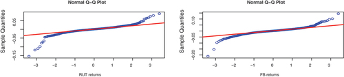
The time series data is further described by plotting the empirical density versus the normal distribution as well as the quantile-quantile(qq) plots for the two indices returns as shown in Figures 1 and 2 Clearly, the plots show that the empirical densities are sharp peaked and are left skewed, that is, they are different from the normal distribution and hence it can be concluded that the data are not normally distributed. This finding is in an agreement with the report by the values of skewness and excess kurtosis from Table 1 which are significantly not equal to those of normal distribution of zero and three.

Figure 1. Empirical densities.

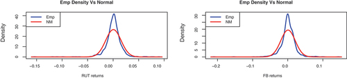
Figure 2. Q-Q plots.

3.3 Empirical findings and discussion

The plots for the RUT and FB stock indices prices and indices returns are presented in Figures 3 and 4, respectively. It is evidenced by Figure 3 that the stock price series have trend implying that the mean and variances of the data are non-constant and as a consequence the data is not stationary.

Figure 3. Adjusted stock index prices.

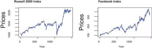
Figure 4. Index returns.

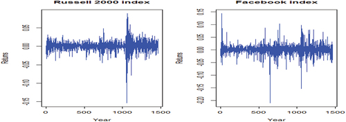
The returns series plots on Figure 4 show the common properties of time series data such as the volatility clustering, leverage effects, leptokurtic distribution and heavy tails. In this connection, the Facebook index returns are characterized by pronounced alternating long spikes compared to the Russell 2000 index returns and these alternating long and short spikes is evidence of volatility clustering in the underlying assets. The non-stationarity of the data calls for the series differencing in order to remove the series dependence before further analysis of the data. The data are therefore differenced once and subjected to statistical tests among them the Ljung-Box, Langrange Multiplier, ARCH effects, Jarque-Bera(JB) and ADF tests in order to confirm that it is stationary and to attain desirable results. The results of these Tests are presented in Table 2. The Ljung-Box test value is significant at 1% significance level for both series which implies that the null hypothesis that the series are not stationary is rejected and hence concludes that the return series are stationary. Moreover, the Ljung-Box and ADF tests imply that the return series have no auto correlations and ARCH effects as well as no unit roots.

Table 3 reports the maximum likelihood parameter estimates for the two indices which are computed according to Equation 28(28) $C(K,T)={\mathbb{E}}^{\mathbb{Q}}[max(X_T-K)|\mathcal{R}]=S_t\varphi (d_1)-e^{-r\tau }K\varphi (d_2)\mathrm{w}\mathrm{h}\mathrm{e}\mathrm{r}\mathrm{e}$(28) and it is clear that the parameters are more or less similar across the two return series. The mean and standard deviations are different across the regimes for the two indices, for instance, the mean in regime 1 is 0.00104 and 0.00163 for Russell 2000 and Facebook indices, respectively. Moreover, the mean ${\mu }_2$ in high-volatility regime is negative for both indices whereas it is positive in the low-volatility regime, that is ${\mu }_1$ is positive. It is evident that in regime 1, the assets has higher returns and low risk compared to lower returns and high risk in regime 2. On the other hand, the probability of switching from the low-volatility regime to the high-volatility regime, estimated at 0.0651 for Russell 2000 and at 0.2087 for Facebook, is significantly different for the two indices. Furthermore, the estimates indicate that the volatility persistence in the low-volatility regime is less in Facebook index than in Russell 2000 index. That is, the probability of switching regime from low-volatility to high-volatility regime is high in Facebook index as compared to Russell 2000 index. In fact, the duration of stay in each regime is computed using the expression $\frac{1}{(1-P_{ii})}\mathrm{f}\mathrm{o}\mathrm{r}i=1,2$ and thus once in regime 1, the process stays there for approximately 15.35 days for Russell 2000 index compared to 4.79 days for Facebook index. In both indices, the process has the tendency of staying in high-volatility regime longer than in low-volatility regime, that is, the process approximately stays in high volatility regime for 58.43 and 16.83 days for Russell 2000 and Facebook indices, respectively.

Table 3. MLE parameter estimates

INDEX	${\tilde{\mu }}_1$	${\tilde{\mu }}_2$	${\tilde{\sigma }}_1$	${\tilde{\sigma }}_2$	${\tilde{P}}_{12}$	${\tilde{P}}_{21}$	AIC	BIC	LogL
RUT	0.001043381	$-$0.001684924	0.009050682	0.028123106	0.06512676	0.01711369	$-$8805.52	$-$8780.357	4404.76
FB	0.001627863	$-$0.002160260	0.01214430	0.03701865	0.208761	0.0594083	$-$7720.164	$-$7695.001	3862.082

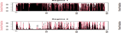
The model log likelihood is higher for Russell 2000 index returns than that of Facebook index returns (estimated at 4404.76 and 3862.082 for RUT and FB returns, respectively), whereas the model AIC and BIC are small for RUT and FB indices returns, respectively. This implies that the RS) model provides a reasonable fit to the Russell 2000 index returns compared with the Facebook index returns. Moreover, Figures 5 and 6 show the smoothed probabilities for the Russell 2000 and Facebook indices returns and clearly the volatility process stays in regime 2 longer most of the periods than in regime 1. That is, although the two regimes are highly persistent, regime two is more persistent than regime one in the two market indices and is expected to continue for approximately 58 and 17 days for RUT and FB indices, respectively, before exiting to regime 1. Furthermore, a comparison of the two markets shows that the regimes dynamics in RUT and FB indices appears rather different.

Figure 5. Smoothed probability for Russell 2000 index.

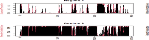
Figure 6. Smoothed probability for Facebook index.

The results presented in Table 3 for the parameter estimates of the Facebook and Russell 2000 indices returns are implemented in Equation 28(28) $C(K,T)={\mathbb{E}}^{\mathbb{Q}}[max(X_T-K)|\mathcal{R}]=S_t\varphi (d_1)-e^{-r\tau }K\varphi (d_2)\mathrm{w}\mathrm{h}\mathrm{e}\mathrm{r}\mathrm{e}$(28) to calculate the European call option prices for some strike prices obtained from the Facebook and Russell 2000 stock indices. Table 4 presents the calculated option prices for 34 and 60 days call options for Russell 2000 and Facebook indices, respectively. This research assumes a risk free-free interest rate of 6% per annum and the initial stock price is 2277.1 and 330.64 for Russell 2000 and Facebook indices, respectively. The calculated call option prices from both the Black-Scholes and RS models are more or less similar for the two market indices. However, the calculated prices from the Black-Scholes (BS) model are slightly closest to the market prices across the two markets. This implies that the BS model gives better results for the Russell 2000 and Facebook indices data sets as compared with the RS model. In addition, the plot of the strike prices versus the estimated call options and the observed option prices in the market indices is presented in Figure 7. The plots indicates similar curve patterns for the two stock indices with the estimated price curve from Black-Scholes model being closer to the observed market price curve than the curve for the RS model. This may imply that the Black-Scholes model gives a better estimated European call options than the RS model for the utilized data sets.

Figure 7. Options.

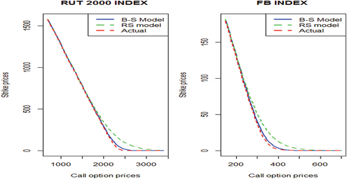
Table 4. Call option prices for Russell 2000 and Facebook indices

		RUSSELL			FACEBOOK
		B-S	RS			B-S	RS
Strike	Market price	Call	Call	Strike	Market price	Call	Call
700	1575.80	1580.901	1580.901	150	179.525	182.112	182.126
1000	1276.30	1282.573	1282.574	160	169.465	172.210	172.264
1050	1225.60	1232.852	1232.854	165	159.550	167.259	167.314
1200	1076.30	1083.688	1083.723	170	155.300	162.309	162.389
1240	1035.80	1043.911	1043.977	175	149.550	157.358	157.474
1250	1025.90	1033.967	1034.044	180	144.650	152.407	152.572
1300	976.00	984.246	984.408	185	144.650	147.457	147.820

Furthermore, the estimated European call option prices from the Black-Scholes and RS models and the observed market option prices are used to compute the Root Mean Square Error (RMSE) in order to establish which model gives better results for pricing the European options. The results of the Root Mean Square Error (RMSE) are presented in Table 5 and it can be seen that the Black-Scholes model has smaller values than the RS model across the two data sets. It is thus implied that the Black-Scholes model gives a better option price prediction than the RS model.

Table 5. RMSE for the black-Scholes and regime-switching models

	RUSSELL 2000 index	FACEBOOK index
B-S	RS	B-S	RS
2.3637	8.9161	11.6971	51.4931

4 Conclusion

A RS model for pricing European call options in a financial market that exhibits structural changes with time is derived in this paper. The model is formulated based on the basis that the underlying asset dynamics are described by a geometric Brownian motion that is modulated by a continuous-time Markov chain with switching regimes. That is, this model allows the volatility to follow a RS process that is governed by a Markov chain process and it is implemented by considering two regimes, that is, the low and high volatility regimes. The model parameters are estimated by utilizing data from the Russell 2000 and Facebook indices and these model parameter estimates are then utilized to compute the European call option prices. The European call option prices reported by the RS model are compared with those that are reported by the Black-Scholes model. Moreover, a comparison of the two models is done in order to establish the model that gives better results in terms of predicting the European call option prices by computing a Root Mean Square Error for each model. This study finds out that across the two market indices, regime 1 is characterized by low risk and high returns whereas regime 2 is characterized by high risk and low returns. The transition probabilities imply that the probability of switching from the low-volatility regime to the high-volatility regime is significantly different across the two market indices and it is higher than the probability of reverting back. That is, the volatility process has the tendency of staying in high-volatility regime longer than it stays in low-volatility regime across the two markets. However, the volatility persistence in the low-volatility regime is less in Facebook index than in Russell 2000 index, that is, the probability of switching regimes from low-volatility to high-volatility regime and vice versa is high in Facebook index as compared to Russell 2000 index. The calculated European call option prices from both the Black-Scholes and RS models are more or less similar for the two market indices. However, the price values reported by the Black-Scholes (BS) model are a bit closer to the market price than that of RS model across the two markets. This implies that the BS model slightly gives better results for the Russell 2000 and Facebook indices data sets as compared with the RS model.

This study focused on developing a RS model for pricing options when the underlying asset dynamics depend on the market regimes. The model formulation is based on a geometric Brownian motion that is governed by a continuous-time Markov chain with two states, and the implementation of the model is done by computing the European call option prices for some chosen stock market indices. Future studies can focus on implementing this model for a case of more than two regimes. Moreover, future studies can consider the application of this model in the American options pricing and draw its performance comparison with that of the Black-Scholes model for both long and short-dated data.

Disclosure statement

No potential conflict of interest was reported by the authors.

Additional information

Notes on contributors

Sebastian Kaweto Kalovwe

Sebastian Kaweto Kalovwe, is a Doctor of Philosophy in Financial Mathematics from the University of Nairobi-Kenya. He also holds Msc in Mathematics (Statistics) from the Catholic University of Eastern Africa. Previously, he has worked as part-time lecturer (for five years) in the school of pure and applied sciences, South Eastern Kenya University (SEKU). Currently, he is a teacher of Mathematics and Physics at Our Lady of Mercy-Mutomo Girls Secondary School, and a part-time lecturer at Strathmore University. His research interest include; applications of stochastic time series models in modeling financial market data, regime switching modeling and Options pricing under regime switching model. Dr. Kalovwe has vast experience in teaching mathematics and research, and has published articles in different peer-reviewed and reputed journals.

References

- Barone-Adesi, G., Engle, R. F., & Mancini, L. (2008). A garch option pricing model with filtered historical simulation. The Review of Financial Studies, 21(3), 1223–19. https://doi.org/10.1093/rfs/hhn031
- Bauwens, L., & Lubrano, M. (1998). Bayesian inference on garch models using the gibbs sampler. The Econometrics Journal, 1(1), C23–46. https://doi.org/10.1111/1368-423X.11003
- Biswas, A., Goswami, A., & Overbeck, L. (2018). Option pricing in a regime switching stochastic volatility model. Statistics & Probability Letters, 138, 116–126. https://doi.org/10.1016/j.spl.2018.02.056
- Bollen, N. P. (1998). Valuing options in regime-switching models. Journal of Derivatives, 6(1), 38–50. https://doi.org/10.3905/jod.1998.408011
- Bollen, N. P., Gray, S. F., & Whaley, R. E. (2000). Regime switching in foreign exchange rates: Evidence from currency option prices. Journal of Econometrics, 94(1–2), 239–276. https://doi.org/10.1016/S0304-4076(99)00022-6
- Bollerslev, T. (1986). Generalized autoregressive conditional heteroskedasticity. Journal of Econometrics, 31(3), 307–327. https://doi.org/10.1016/0304-4076(86)90063-1
- Buffington, J., & Elliott, R. J. (2002). American options with regime switching. International Journal of Theoretical and Applied Finance, 5(05), 497–514. https://doi.org/10.1142/S0219024902001523
- Cai, J. (1994). A markov model of switching-regime arch. Journal of Business & Economic Statistics, 12(3), 309–316. https://doi.org/10.1080/07350015.1994.10524546
- Deelstra, G., Latouche, G., & Simon, M. (2020). On barrier option pricing by erlangization in a regime-switching model with jumps. Journal of Computational and Applied Mathematics, 371, 112606. https://doi.org/10.1016/j.cam.2019.112606
- Dieobold, F. X. (1986). Modeling the persistence of conditional variances: A comment. Econometric Reviews, 5(1), 51–56. https://doi.org/10.1080/07474938608800096
- Duan, J. C. (1995). The garch option pricing model. Mathematical Finance, 5(1), 13–32. https://doi.org/10.1111/j.1467-9965.1995.tb00099.x
- Duan, J. C., Popova, I., & Ritchken, P. (2002). Option pricing under regime switching. Quantitative Finance, 2(2), 116. https://doi.org/10.1088/1469-7688/2/2/303
- Duan, J. C., & Zhang, H. (2001). Pricing hang seng index options around the asian financial crisis–a garch approach. Journal of Banking & Finance, 25(11), 1989–2014. https://doi.org/10.1016/S0378-4266(00)00166-7
- Engle, R. F. (1982). Autoregressive conditional heteroscedasticity with estimates of the variance of united kingdom inflation. Econometrica: Journal of the Econometric Society, 50(4), 987–1007. https://doi.org/10.2307/1912773
- Godin, F., & Trottier, D. A. (2019). Option pricing under regime-switching models: Novel approaches removing path-dependence. Insurance, Mathematics & Economics, 87, 130–142.
- Godin, F., & Trottier, D. A. (2021). Option pricing in regime-switching frameworks with the extended girsanov principle. Mathematics and Economics.
- Gray, S. F. (1996). Modeling the conditional distribution of interest rates as a regime-switching process. Journal of Financial Economics, 42(1), 27–62. https://doi.org/10.1016/0304-405X(96)00875-6
- Hamilton, J. D. (1989). A new approach to the economic analysis of nonstationary time series and the business cycle. Econometrica: Journal of the Econometric Society, 57(2), 357–384. https://doi.org/10.2307/1912559
- Hamilton, J. D. (1990). Analysis of time series subject to changes in regime. Journal of Econometrics, 45(1–2), 39–70. https://doi.org/10.1016/0304-4076(90)90093-9
- Hamilton, J. D., & Susmel, R. (1994). Autoregressive conditional heteroskedasticity and changes in regime. Journal of Econometrics, 64(1–2), 307–333. https://doi.org/10.1016/0304-4076(94)90067-1
- Hardy, M. R. (2001). A regime-switching model of long-term stock returns. North American Actuarial Journal, 5(2), 41–53. https://doi.org/10.1080/10920277.2001.10595984
- Jarque, C. M., & Bera, A. K. (1980). Efficient tests for normality, homoscedasticity and serial independence of regression residuals. Economics Letters, 6(3), 255–259. https://doi.org/10.1016/0165-1765(80)90024-5
- Kirkby, J. L., & Nguyen, D. (2020). Efficient asian option pricing under regime switching jump diffusions and stochastic volatility models. Annals of Finance, 16(3), 307–351. https://doi.org/10.1007/s10436-020-00366-0
- Lamoureux, C. G., & Lastrapes, W. D. (1990). Persistence in variance, structural change, and the garch model. Journal of Business & Economic Statistics, 8(2), 225–234. https://doi.org/10.1080/07350015.1990.10509794
- Lin, S., & He, X. J. (2020). A regime switching fractional black–Scholes model and european option pricing. Communications in Nonlinear Science & Numerical Simulation, 85, 105222. https://doi.org/10.1016/j.cnsns.2020.105222
- Mitsui, H. (2000). An analysis of nikkei 225 option pricing by a garch model. Gendai-Finance, 7, 57–73.
- Mitsui, H., & Satoyoshi, K. (2010). Empirical study of nikkei 225 option with markov switching garch model. Asia-Pacific Financial Markets.
- Mitsui, H., & Watanabe, T. (2003). Bayesian analysis of garch option pricing models. Journal Japan Statistical Society(japanese Issue), 33, 307–324.
- Nasri, B. R., Remillard, B. N., & Thioub, M. Y. (2020). Goodness-of-fit for regime-switching copula models with application to option pricing. Canadian Journal of Statistics, 48(1), 79–96. https://doi.org/10.1002/cjs.11534
- Siu, T. K., Tong, H., Yang, H. (2004). On pricing derivatives under garch models: A dynamic gerber-shiu approach. North American Actuarial Journal, 8(3), 17–31. https://doi.org/10.1080/10920277.2004.12254408
- Yao, D. D., Zhang, Q., & Zhou, X. Y. (2006). A regime-switching model for european options. In Stochastic processes, optimization, and control theory: Applications in financial engineering, queueing networks, and manufacturing systems (pp. 281–300). Springer.