Greenspan’s adherence to the Taylor rule: examining Federal Reserve chairmen policy regimes and deviations from the Taylor rule

Abstract

This paper examines the relationship between Federal Reserve policy and the Taylor rule, a commonly used model for guiding monetary policy. The study analyzes the deviation of the actual Federal Funds Rate from the Taylor Rule model during distinct structural changes, using real-time macroeconomic data available to the Fed at the time of their interest rate decision. The research focuses on whether former Fed chair Alan Greenspan’s policies from 2003 to 2006, which have been linked to the housing bubble, were deviant from the Taylor Rule. The findings show that there isn’t sufficient statistical evidence to support this claim, and a machine learning text analysis of the Federal Open Market Committee transcripts confirms the presence of only one regime during this period. These results contribute to the existing literature on monetary policy and its impact on the economy, providing valuable insights into the relationship between Federal Reserve policy and the Taylor Rule.

Keywords:

• Taylor rule
• Alan Greenspan
• monetary policy regimes
• machine learning
• text clustering

Jel Classification:

• E44
• E52

1. Introduction

Since the end of the inflationary episode in the 1970s, the U.S. has experienced a significant reduction in the volatility of GDP growth (with the exception of the 2008 recession) and only a moderate amount of yearly inflation (with the exception of 2021−present). This has prompted extensive empirical research to assess why economic conditions have changed so dramatically. A possible explanation is that the U.S. Federal Reserve has changed the decision-making process that determines the federal funds rate. Consequently, there is a growing interest in modeling the process by which this decision is made and determining whether this process has changed over time.

Various efforts have been made to model the decision-making process of the Federal Reserve on the federal funds rate question, with the ”Taylor Rule” emerging as the clear winner. Named after its creator, John Taylor, the rule is presented as a simple equation that specifies how the federal funds rate should be set based on three variables: the equilibrium real interest rate, the deviation of real GDP from a target, and the inflation gap. The original rule from Taylor (1993) stipulates that the federal funds rate, $i_t$, should be set in response to the equilibrium real interest rate, $r^{\ast }$, the deviation of real GDP from a target, $y_t$, and the inflation gap (the difference between the observed inflation, ${\pi }_t$, and the target inflation rate, $\pi$*) according to

(1) $i_t=r^{\ast }+{\pi }_t+{\lambda }_1{y}_t+{\lambda }_2({\pi }_t-{\pi }^{\ast }).$(1)

Taylor suggests $y_t=100(Y_t-Y_t^{\ast })/Y_t^{\ast }$, i.e. the percent difference between real output, $Y_t$, and trend or potential output $Y_t^{\ast }$. Including Taylor’s suggestion for the parameter values and targets, the rule becomes

(2) $i_t=2+{\pi }_t+0.5y_t+0.5({\pi }_t-2).$(2)

Taylor initially presented the rule at the 1992 Carnegie-Rochester Conference as an empirical regularity, but its descriptive power has gradually transformed the formula into a policy prescription, particularly by Taylor himself. The rule has been used to evaluate the US Federal Reserve’s monetary policy over various periods. For instance, Taylor (2007, 2009) used the rule named after him to argue that monetary policy was “too loose” from 2003 to 2006 compared to the experience of the previous few decades and played a role in the formation of the housing bubble by making housing finance cheap and attractive, thereby contributing to the boom-bust cycle in housing starts. Taylor’s arguments are based on evaluating Greenspan’s adherence to a Taylor rule that uses final values of the output gap and inflation rate.

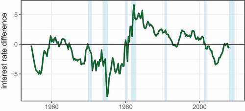
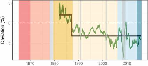
Figure 1 displays the actual federal funds rate and the one suggested by the Taylor Rule with final values of the output gap and inflation rate. Plotting the difference between the actual federal funds rate and that suggested by Taylor Rule in Figure 2, we can see the dip from 2003 to 2006 in the series that constitutes the “loose” period in Greenspan’s tenure that is contentious for Taylor.

Figure 1. St. Louis fed Taylor rule.

Notes: The figure shows the federal funds rate (red), along with the implied federal funds rate from the original formulation of the Taylor Rule (blue), as calculated by The St. Louis Federal Reserve. The vertical bars denote recessions as defined by the NBER. Both series are based on quarterly data, with the federal funds rate data points representing the quarterly average of the effective federal funds rate.

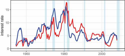
Figure 2. $i_{FedFund,t}-i_{Taylor,t}:$1954–2008.

Notes: The figure shows the difference between the quarterly average federal funds rate, $i_{FedFund}$ and the federal funds rate implied by the Taylor Rule, $i_{Taylor}$. The series is quarterly from 1954:Q3 to 2008:Q1.

However, research in this area has been subject to some controversy due to different methods of measuring inflation. Alex et al. (2019) argue that the period from 2000 to 2007 was inconsistent with the Taylor Rule, due to the use of the real-time GDP deflator as the measure of inflation rather than the vintage core-PCE series the Federal Reserve was using at the time. The author argues that this inconsistency highlights the importance of using accurate measures of inflation when implementing the Taylor Rule.

Similarly, Orphanides and Wieland (2008) conclude that policy actions from 1988 to 2007 (Greenspan’s tenure) have been consistent with a stable Taylor rule. They confirm that many of the apparent deviations of the federal funds rate from the prescriptions of an outcome-based Taylor rule may actually be the result of the policymakers’ systematic responses to projections of output gap and inflation as opposed to recent economic data, as confirmed by the authors. Orphanides (2001, 2002) emphasize the necessity of evaluating monetary policy with rules based on real-time data, and one should judge the federal funds rate policy based on the information available to the policymakers at the time of policy decision rather than ex-post revised data, which is only available much later. In fact, Mehra and Sawhney (2010) find that applying a forward-looking Taylor Rule using real-time inflation data reduces much of the gap between the federal funds rate and the Taylor Rule recommendation in 2003–2006.

Despite the existing research, questions remain about the consistency of the Taylor Rule and the Federal Reserve’s adherence to it. This paper adds to this literature in two fronts. First, we perform a data-based determination of regime changes in U.S. monetary policy by employing the methods of Alex et al. (2019), but using the insight of Mehra and Sawhney (2010) that it is necessary to use real-time core-PCE as the measure of inflation in the Taylor Rule post-2004, rather than CPI or the GDP deflator thereby reflecting the series used by the Federal Reserve at the time. We employ a standard non-forward-looking version of Taylor’s (Taylor, 1993, 1999) decision model of the federal funds rate, the version of the Taylor Rule suggested by the St. Louis Federal Reserve (Equation 2(2) $i_t=2+{\pi }_t+0.5y_t+0.5({\pi }_t-2).$(2) ), where the potential GDP series comes from the Congressional Budget Office (CBO) model potential GDP in the U.S. Second, we add to the literature by confirming our more standard time series regimes switching analysis with a machine learning text analysis approach to determine regime changes in monetary policy. In this methodology, the monetary policy regime is determined by which cluster of related transcripts a particular FOMC meeting is determined to belong. This provides an independent method of finding policy regimes. However, we can only identify monetary policy regimes over a more limited period (since machine-readable FOMC meeting transcripts were not available until 1979). Due to the lack of availability of the full meeting transcripts, Greenspan’s era can only be compared to Volcker’s chairmanship period.

The rest of the paper is organized as follows. Section 2 discusses the literature on previous regime identification as well as on the application of machine learning techniques on FOMC transcripts. Section 3 reviews the Taylor Rule and the construction of deviation series with the data available to the Fed at the time of their decisions. Section 4 discusses the empirical regime detection methodologies, Section 5 presents the empirical results, and Section 6 concludes.

2. Previous literature

Regime changes in U.S. monetary policy have been extensively studied using a variety of methodologies, each with its own strengths and limitations. Table 1 summarizes the most common approaches in the literature. Early approaches, such as the binary indicator variable method proposed by Hamilton (1989), were limited to only two regimes and did not account for changes in the economy over time. Sims (1992) proposes a more general approach to identifying and estimating changes in the parameters of a dynamic model. Compared to Hamilton’s (1989) Markov-switching model, which assumes a fixed number of regimes, Sims (1992) VAR approach does not require a pre-specified number of regimes. Instead, the number of regimes can be determined endogenously based on the data, making it a more data-driven approach. However, these models relied on assumptions about the structure of the economy and faced challenges in identifying relevant shocks. To address these limitations, researchers such as Fair (2001), and Judd and Rudebusch (1998) modified the SVAR model to allow for more flexible identification schemes and better incorporation of economic theory.

Table 1. Summary of literature review on identifying and analyzing monetary policy regimes

Methodology	Features	References
Binary variable method	Limited to only two regimes and did not account for changes in the economy over time	Hamilton (1989)
Structural VAR	Allow for multiple regimes, but still assumed a fixed and known number of regimes	Sims (1992), Judd and Rudebusch (1998), Clarida et al. (1999), Fair (2001), Sims and Zha (2006)
Time-varying parameter models	Allow for changes in the model parameters over time, but have their own limitations	Primiceri (2005), Boivin (2006)
Bayesian methods	Allow for more flexible modeling of uncertainty and can produce more accurate estimates of the model parameters but require specifying prior distributions for the model parameters	Timothy and Sargent (2005), Murray et al. (2015) and Alba and Wang (2017)
Structural change model with regime switching	Identify regimes and fit OLS regressions for each regime.	Alex et al. (2019)
Machine learning methods	Use methods such as sentiment analysis, neural network and topic modelling to estimate changes in monetary policy regimes, allowing for more flexible modeling of complex relationships between variables.	Shapiro and Wilson (2022), Handlan (2021), and Hansen and McMahon (2016)

A typical method is to choose regime dates based on some known features and history of the available data and then use tests of parameter constancy, e.g., Chow tests, to justify the dates chosen. However, as Hansen (2001) observes, if the breakpoints are not known $apriori$, then the Chi-squared critical values for the Chow test are inappropriate. Using known features of the data (e.g., the Volcker policy experiment of 1979–82) to determine breakpoints can make these candidate break dates endogenously correlated with the actual data, leading to incorrect inferences about the significance of those candidate break dates. Furthermore, not all of the parameters or targets necessarily change at the same date. Fitting values to the policy parameters on the output and inflation gap, ${\lambda }_1$ and ${\lambda }_2$ in equation (1)(1) $i_t=r^{\ast }+{\pi }_t+{\lambda }_1{y}_t+{\lambda }_2({\pi }_t-{\pi }^{\ast }).$(1) , with an OLS model, such as

(3) $i_t=\alpha +{\beta }_1{y}_t+{\beta }_2({\pi }_t-{\pi }^{\ast })+{\in }_t,$(3)

provides less than reliable parameter estimates if the regime includes few data, as is the case with potential Volcker policy experiment.

Boivin (2006) attempt to address some of these issues by using a Time-Varying Parameter model that assumes that policy parameters are time series which follow drift-less random walks. This is the Kalman filter model of Cooley and Prescott (1976), and all the parameters in the model can be estimated jointly by maximum likelihood estimation. However, when the variance of the policy parameter time series is small, the parameters can only change slowly over time, and policy regime shifts may not be visible. Boivin (2006) deals with this problem in an ad hoc manner but still fails to identify discrete regimes that align with the terms of particular Federal Reserve Chairs. He finds only a gradual shift in the Taylor Rule policy parameters until around 1982, the start of the Great Moderation.

Timothy and Sargent (2005) use a Bayesian Markov-switching VAR model to identify changes in the conduct of monetary policy and their effects on key macroeconomic variables. Their model allows for different regimes, each with its own set of parameters and error variances, to capture the possibility that the relationship between policy and macroeconomic outcomes may change over time. Sims and Zha (2006) improve upon the earlier studies by introducing a new approach to modeling regime-switching dynamics that allow for continuous and endogenous shifts in the behavior of both policymakers and the economy. Murray et al. (2015) use Markov-Switching models to identify regimes from 1965 onward and find that the Taylor parameters are mostly consistent, except for 1973–1974 and 1980–1985. Alba and Wang (2017) also identify monetary regimes between 1973 and 2014 using a k-state Markov regime-switching model and find 2001Q2 to 2005Q4 to be mostly consistent with the Taylor Rule “low discretionary regime,” and 2006Q1 to 2007Q4 to be completely consistent with the Taylor Rule, which is broadly consistent with other findings, despite their use of the GDP deflator instead of the CPI and core-PCE post-July 2004. These methods allow for more flexible modeling of uncertainty and can produce more accurate estimates of the model parameters but require specifying prior distributions for the model parameters.

The work closest to ours, Alex et al. (2019), use the Bai and Perron (2003a, 2003b) structural change model to identify regimes and fit OLS regressions similar to equation (3)(3) $i_t=\alpha +{\beta }_1{y}_t+{\beta }_2({\pi }_t-{\pi }^{\ast })+{\in }_t,$(3) for each regime to check for significant deviations from the expected parameters on the inflation and output gap. However, their conclusion that the 2000–2007 period had significantly different parameters than the standard Taylor rule is dependent on using the GDP deflator as the measure of inflation rather than real-time core PCE, as shown in other studies.

Recently, machine learning methods, specifically text analysis, on central bank communication have been on the rise to study monetary policy. Hansen and McMahon (2016) use topic modeling to analyze the effect of forward guidance on macroeconomic aggregates. Shapiro and Wilson (2022) use sentiment analysis on FOMC transcripts to estimate the objectives of central bank preferences. They find that the FOMC’s implicit inflation target was roughly 1.5 percent, significantly below the assumed value of 2 percent. Handlan (2021) uses neural networks for text analysis on FOMC meeting statements to generate “monetary policy shocks” series and find that the wording of the statements accounted for more variation in federal funds futures (FFF) prices than target federal funds rate change announcements. She also finds that the impact of forward guidance on real interest rates is twice as large when using these text-based shock series compared to other measures, such as changes in FFF prices. To our knowledge, ours is the first paper to identify different Federal Reserve decision framework regimes using machine learning methods.

3. Data

The federal funds rate, inflation, unemployment, and output time series come from the U.S. Federal Reserve Bank of St. Louis’ FRED database. The potential output series in the initial Taylor Rule comes from the Congressional Budget Office and is imported from the St. Louis Federal Reserve. The St. Louis Federal Reserve Taylor Rule series runs quarterly for 54 years from 1954:Q3–2008:Q4. For the the real-time Taylor Rule we create, the Federal Reserve Bank of Philadelphia has a Real-Time Data Set only available from 1965 onward, limiting our real-time Taylor Rule series to run from 1965 to 2008. We also obtain FOMC transcripts from the Board of the Governors of the Federal Reserve System website for the text clustering portion of the paper, but transcripts of the meetings are only available from 1979 to present (Board of Governors of the Federal Reserve System, 2021).

3.1. Real time taylor rule

The Taylor Rule assumes that policymakers know, and can agree on, the size of the output gap. However, measuring the output gap is very difficult and FOMC members typically have different judgments. In addition, since the FOMC meets eight times per year, assessing the Taylor Rule consistency of the FOMC using quarterly data could be misleading. It is fairer to assess the consistency of the federal funds rate with Taylor Rule using monthly data that was available to the committee at the time of their meeting. Instead of attempting to interpolate quarterly output and potential output data with a method similar to Sims (1980), we choose to approximate the output gap using Okun’s law,

(4) $y_t=-c(U_t-U_t^{\ast }).$(4)

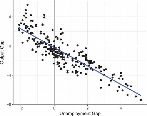
Equation 4(4) $y_t=-c(U_t-U_t^{\ast }).$(4) is the gap version of Okun’s “rule of thumb” as presented in Abel et al. (2005). For the period of 1954–2008, the slope of the line is −1.26 (Figure 3). This suggests that the Taylor Rule on a monthly frequency is

Figure 3. Gap version of Okun’s law 1954–2008.

Notes: The figure shows the regression results based on Equation 4(4) $y_t=-c(U_t-U_t^{\ast }).$(4) , regressing the Output gap on the Unemployment gap using quarterly Output and Unemployment. The estimated slope for the period is −1.26, rather that the −2 estimated from Okun’s original data.

(5) $i_t=2+{\pi }_t+0.5(-1.26(U_t-U_t^{\ast }))+0.5({\pi }_t-2).$(5)

The Natural Rate of Unemployment, $U_t^{\ast }$ from the U.S. Congressional Budget Office must still be interpolated from quarterly to monthly frequency, producing the series shown in Figure 4. However, this version of the Taylor rule also has the advantage of being able to use the historical values of inflation (${\pi }_t$) and unemployment ($U_t$) values that were the estimates at the time of the FOMC meeting, rather than the revised series. This data is available from the Federal Reserve Bank of Philadelphia’s Real-Time Data Set from 1965 onward. The final version of “real-time” Taylor rule is

Figure 4. Monthly natural rate of unemployment.

Notes: The figure displays the U.S. Congressional Budget Office Short-Term Natural Rate of Unemployment, $U_t^{\ast }$, interpolated from quarterly to monthly frequency.

(6) $i_t=2+{\pi }_t-0.63(U_t-U_t^{\ast })+0.5({\pi }_t-2).$(6)

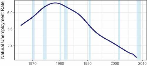
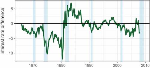
Figure 5 shows the difference between the monthly average federal funds rates and the federal funds rate implied by the Taylor rule in Equation 6(6) $i_t=2+{\pi }_t-0.63(U_t-U_t^{\ast })+0.5({\pi }_t-2).$(6) . The series has 507 monthly data points from 1965 to 2008. The Taylor rule residual series is still biased (mean = −1.25%) toward a higher interest rate than the Taylor rule suggests (i.e. a bias toward less permissive monetary policy). The “Real-Time” series is obviously much closer to being stationary, but is still not consistent with the single Taylor rule over the entire period.

Figure 5. Real-Time $i_{FedFund,t}-i_{St.Louis,t}$, 1965–2008.

Notes: The figure shows the difference between the monthly average federal funds rate, $i_{FedFund}$ and the federal funds rate implied by the monthly version of the Taylor Rule, $i_{TaylorMonthly}$, in Equation 6(6) $i_t=2+{\pi }_t-0.63(U_t-U_t^{\ast })+0.5({\pi }_t-2).$(6) . The inflation and unemployment estimates are the initial series available at the time of the Federal Reserve meeting, acquired from the Federal Reserve Bank of Philadelphia’s Real-Time Data Set, rather than the revised series published by St. Louis Federal Reserve. The series runs from October 1965 to December 2007.

In February 2000, CPI was replaced by the personal consumption expenditures (PCE) deflator as the preferred FOMC measure of inflation. From July 2004 onward, the Fed began targeting the core-PCE price index that excludes food and energy prices. As Mehra and Sawhney (2010) point out, these adjustments reduce much of the apparent Greenspan deviation from the Taylor Rule from 2003 to 2006.

4. Empirical methodology

The Tukey Honest Significant Difference Test is a single-step multiple comparison procedure that determines if sample means are significantly different from each other simultaneously. The test assumes that the observations are independent with and among groups, and there is homogeneity in within-group variance across the groups. Since we first wish to test whether Greenspan’s tenure is distinguishable from the other Fed Chairmen on an aggregate basis, this is a suitable procedure to perform before attempting to identify regimes with an agnostic statistical procedure.

It is easiest to judge the break points, however, using the multiple mean model, even though there is autocorrelation in the federal funds rate-Taylor rule difference series. It is also useful to think of the FOMC monetary policy as having an unbiased error in relation to the Taylor rule in each regime. Using this assumption and using the methodology of Bai and Perron (1998, 2003a, 2003b), we fit multiple mean equations to the series and find the points in time that minimize the residual sum of squares for the chosen number of breakpoints. The optimal number of breakpoints is three, based on the Schwarz Information Criterion (SIC).

Another useful way to find the hidden regimes in monetary policy is with the Markov switching model of Hamilton (1989), one of the most popular nonlinear time series models in the literature. This model involves multiple structures (equations) that can characterize the time series behaviors in different regimes. By permitting switching between these structures, this model is able to capture more complex dynamic patterns. A novel feature of the Markov switching model is that the switching mechanism is controlled by an unobservable state variable that follows a first-order Markov chain. In particular, the Markovian property regulates that the current value of the state variable depends on its immediate past value. As such, a structure may prevail for a random period, and it will be replaced by another structure when a switching takes place. This is in sharp contrast with the random switching model of Quandt (1972) in which the events of switching are independent over time. The original Markov switching model focuses on the mean behavior of variables. This model and its variants have been widely applied to analyze economic and financial time series (c.f. Diebold et al. (1994); Engel (1994); Engel and Hamilton (1990); Hamilton (1988, 1989); Filardo (1994); Garcia and Perron (1996); Ghysels (1994); Goodwin (1993); C.J. Kim and Nelson (1998); M.J. Kim and Yoo (1995); Lam (1990); Sola and Driffill (1994); Schaller and Van Norden (1997); Athanasios and Williams (2003); Westelius (2007)). In traditional Markov switching models, the regime probabilities are exogenous and are usually estimated using maximum likelihood estimation methods. However, Yoosoon et al. (2017) extend the regime switching methodology by allowing the Markov chain determining regimes to be endogenous, implying that the switching probabilities depend on the state of the underlying process. Similarly, Svensson (2017) uses a regime-switching model with an endogenous Markov chain to analyze the effectiveness of an approach that involves setting interest rates based on forecasts of future inflation and output rather than relying on a specific rule or model.

Let $s_t$ denote the unobservable state variable. The switching model for the Taylor Rule deviation ($i_{Taylor}$) series we consider involves three regimes,

(7) $i_{Taylor}=\left\{\begin{array}{cc}{\alpha }_0+{\in }_t,{\in }_t\sim N(0,{\sigma }_1^2),& s_t=0\\ {\alpha }_1+{\in }_t,{\in }_t\sim N(0,{\sigma }_2^2),& s_t=1\\ {\alpha }_2+{\in }_t,{\in }_t\sim N(0,{\sigma }_3^2),& s_t=2.\end{array}\right.$(7)

This model could be thought of as representing three states of monetary policy relative to the Taylor Rule, where “tight”, “loose”, and “other” are three hidden states which each $s_t$ might represent. This formulation allows for the presence of different conditional variances across regimes, and so is a less restrictive version of the methodology of Bai and Peron.

When $s_t$ are independent Bernoulli random variables, it is the random switching model of Quandt (1972). In the random switching model, the realization of $s_t$ is independent of the previous and future states. This would imply that the deviation from the Taylor rule belongs to one of several regimes randomly, which is not consistent with the concept of the hidden state being the particular Fed chairman, who is likely not changing policy stances from month to month randomly. Suppose instead that $s_t$ follows a first-order Markov chain with the following transition matrix:

(8) $P=\left[\begin{array}{ccc}{p}_{00}(s_t=0|s_{t-1}=0)& p_{01}(s_t=1|s_{t-1}=0)& p_{02}(s_t=2|s_{t-1}=0)\\ p_{10}(s_t=0|s_{t-1}=1)& p_{11}(s_t=1|s_{t-1}=1)& p_{12}(s_t=2|s_{t-1}=1)\\ p_{20}(s_t=0|s_{t-1}=2)& p_{21}(s_t=1|s_{t-1}=2)& p_{22}(s_t=2|s_{t-1}=2),\end{array}\right]$(8)

where $p_{ij}$ (i,j = 0,1,2) denote the transition probabilities of $s_t=j$ given that $s_{t-1}=i$ so that the transition probabilities satisfy $p_{i0}+p_{i1}+p_{i2}=1$. The transition probabilities determine the persistence of each regime.

4.1. Text analytics

We also employ a machine learning procedure, specifically text clustering, to the FOMC transcripts and find evidence that the Greenspan tenure post-2000 was in large part consistent with his tenure in pre-2000. In particular, we employ k-means clustering on the FOMC transcripts to identify different monetary policy regimes. The idea with clustering is to categorize a set of texts in such a way that texts in the same cluster are more similar to each other than texts in other clusters by applying machine learning and natural language processing techniques. As such, the k-means clustering algorithm takes in a set of FOMC transcript texts as inputs and yields the list of detected clusters, where each cluster is taken to represent a distinct policy regime.

Before we describe the clustering technique, we provide a brief discussion of text pre-processing. In order to apply machine learning techniques, we need to convert the transcript texts to numerical vectors. We split the texts into single words and two-word phrases by removing numbers, punctuation, symbols, and white spaces. We also remove the names of the FOMC members present during a meeting to ensure that our clustering will not be driven solely by the names of the members. We then count the frequency of single-word and two-word phrases within the transcript and normalize the frequencies by the size of the document. As a final step, we weight the terms that occur in the majority of documents with diminishing importance. We use the tf-idf scheme by Salton and McGill (1983) to obtain weights for each term.¹ Essentially, each FOMC transcript is uniquely represented by a vector of normalized frequencies of single words and two-word phrases which can now be employed in the clustering exercise.

The k-means clustering algorithm requires the user to first specify the number of clusters before grouping the FOMC transcripts into those clusters. We use a widely used method called the “elbow method” to determine the number of clusters. Appendix A.2 discusses the k-means clustering algorithm in detail.

4.2. Optimal number of clusters

To apply the “Elbow Method” of determining the optimal number of clusters, the within-group sums of squares is plotted against the number of clusters. If the plot resembles an arm, then the “elbow” on the arm is the appropriate number of clusters, i.e. where the inflection point of the curve exists. This inflection point occurs where the marginal benefit (in terms of a lower sum of squares error) from adding additional clusters begins to diminish, and is thus the point where there is a balance between model parsimony and fit to the data. Figure A1 in the Appendix (Appendix A.3) plots the within-group sum of squares against the number of clusters. The appropriate number of cluster as suggested by the elbow method is anywhere between 3 and 4. Beyond the 4 clusters, the within-group sums of square do not fall much. We do present results for when FOMC transcripts are split into 2, 3, 4, and 5 regimes, but it turns out that the results are quite consistent across all clusters.

5. Results

Table 2 and Table 3 demonstrate that, regardless of which form of the Taylor Rule is utilized, Alan Greenspan’s tenure as Federal Reserve Chair is significantly closer to the Taylor Rule in aggregate than any previous Chairman, with the exception of Bernanke. The absolute value of Greenspan’s deviation is the smallest, and there is a statistically significant difference in Greenspan’s mean deviation from the Taylor Rule and the average deviation of all other Chairmen, except for Bernanke.

Table 2. Tukey HSD:St. Louis rule

	Difference	Lower	Upper	P-value
Bernanke-Greenspan	−0.835	−1.703	0.034	0.069
Burns-Greenspan	−2.990	−3.861	−2.118	0
Martin-Greenspan	−1.218	−2.309	−0.127	0.017
Miller-Greenspan	−4.450	−6.198	−2.701	0
Volcker-Greenspan	2.568	1.696	3.439	0
Burns-Bernanke	−2.155	−3.182	−1.128	0.00000
Martin-Bernanke	−0.383	−1.602	0.835	0.968
Miller-Bernanke	−3.615	−5.446	−1.785	0.00000
Volcker-Bernanke	3.402	2.375	4.429	0
Martin-Burns	1.772	0.551	2.992	0.0004
Miller-Burns	−1.460	−3.292	0.372	0.219
Volcker-Burns	5.557	4.528	6.587	0
Miller-Martin	−3.232	−5.178	−1.286	0.00002
Volcker-Martin	3.785	2.565	5.006	0
Volcker-Miller	7.017	5.185	8.849	0

Notes: The table shows the results of the Tukey Honest Significant Difference multiple comparison procedure for testing the difference in mean Federal Reserve Chairman deviance from the original version of the Taylor Rule. Greenspan has a significantly tighter adherence to the Taylor Rule than every former Chairman other than Bernanke.

Table 3. Tukey HSD: Bernanke rule

	Difference	Lower	Upper	P-value
Bernanke-Greenspan	0.297	−0.636	1.231	0.965
Burns-Greenspan	−2.475	−3.412	−1.538	0
Martin-Greenspan	−2.341	−3.513	−1.168	0.00000
Miller-Greenspan	−4.222	−6.101	−2.342	0
Volcker-Greenspan	3.974	3.037	4.911	0
Burns-Bernanke	−2.773	−3.876	−1.669	0
Martin-Bernanke	−2.638	−3.948	−1.328	0.00000
Miller-Bernanke	−4.519	−6.487	−2.551	0
Volcker-Bernanke	3.676	2.573	4.780	0
Martin-Burns	0.135	−1.178	1.447	1.000
Miller-Burns	−1.747	−3.716	0.223	0.121
Volcker-Burns	6.449	5.342	7.556	0
Miller-Martin	−1.881	−3.973	0.211	0.110
Volcker-Martin	6.314	5.002	7.627	0
Volcker-Miller	8.196	6.226	10.165	0

Notes: The table shows the results of the Tukey Honest Significant Difference multiple comparison procedure for testing the difference in mean Federal Reserve Chairman deviance from the Bernanke version of the Taylor Rule. Again, Greenspan has a significantly tighter adherence to the rule than every former Chairman besides Bernanke.

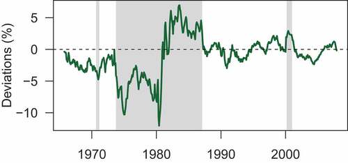
Figure 6 displays the federal funds rate-Taylor Rule difference series with separate means for each regime. The first regime that the Bai and Peron’s statistical procedure identified covers the chairmanship tenures of William Martin (1951–1970) and Arthur Burns (1970–1978), from the start of the series until 1973. This was a period of very loose monetary policy, perhaps influenced by President Nixon’s threats of taking away Federal Reserve independence. Burns’ monetary policy under the Ford presidency after the breakpoint in 1973 was even looser and less consistent with the Taylor rule.

Figure 6. Fitted regimes with Fed Chairman tenure periods, 1965–2008.

Notes: The figure shows the monthly series representing the monthly deviation from the Taylor Rule (green), along with the conditional means from the Bai and Perron structural break methodology (brown). The tenure of each Federal Reserve chairman is represented by the shaded background regions. Martin (pink), Burns (salmon), Volcker (yellow), Greenspan (tan), Bernanke (light blue), and Yellen (dark blue) are denoted. Vertical grey bars represent the NBER recession periods.

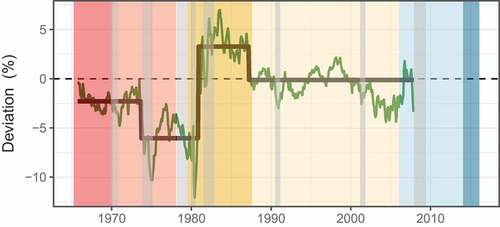
The second breakpoint in 1980 is somewhat expected and agrees with the drifting output and inflation gap evidence from Boivin (2006). The chairmanship of Paul Volcker (1979–1987) exhibits a clear breakpoint in Taylor rule consistency to a regime of tight monetary policy in November of 1980 until the end of tenure, a result that is not surprising given that the Federal Reserve targeted non-borrowed reserve levels rather than the federal funds rate during 1979–1982. The high interest rate period continued until the end of Volcker’s tenure in 1987, as the Fed continued to battle stagflation by first taming inflation (an emphasis on the inflation gap over the output gap in the standard Taylor rule).

Alan Greenspan’s tenure from 1987 to 2006 was remarkably consistent with the Taylor Rule, regardless of whether the shift from targeting core CPI to core PCE in 2000 is reflected in the Taylor Rule (Figure 7). The conditional mean deviation of Greenspan’s tenure is approximately zero, in either case, as Figures 6 and 7 indicate. However, as Figure 8 shows, Greenspan apparently did not account for inflation expectations in his decision-making, since when his inflation gap is calculated using the University of Michigan 1-year inflation expectations survey, his conditional mean policy stance is consistently “loose”. Greenspan’s tenure is still quite distinct from Volcker’s even when using inflation expectations in the Taylor rule.

Figure 7. Fitted Regimes using PCE rather than CPI inflation target from 2000 to 2008.

Notes: The figure shows the monthly series representing the monthly deviation from the Taylor Rule (green) corrected for the use of PCE as the preferred measure of inflation beginning in 2000, along with the conditional means from the Bai and Perron structural break methodology (brown). The tenure of each Federal Reserve chairman is represented by the shaded background regions. Martin (pink), Burns (salmon), Volcker (yellow), Greenspan (tan), Bernanke (light blue), and Yellen (dark blue) are denoted. Vertical grey bars represent the NBER recession periods.

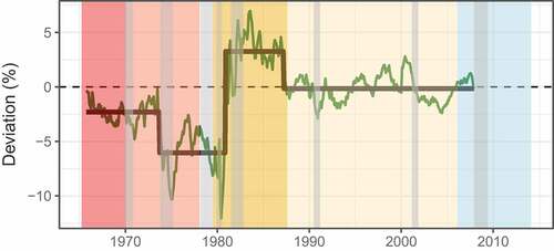
Figure 8. Fitted regimes using university of michigan 1-year inflation expectations for the inflation gap rather than CPI or PCE from 1982 to 2015.

Notes: The figure shows the monthly series representing the monthly deviation from the Taylor Rule (green) using the University of Michigan 1-year inflation expectations survey to calculate the inflation gap, along with the two conditional means from the Bai and Perron structural break methodology (brown). The tenure of each Federal Reserve chairman is represented by the shaded background regions. Martin (pink), Burns (salmon), Volcker (yellow), Greenspan (tan), Bernanke (light blue), and Yellen (dark blue) are denoted. Vertical grey bars represent the NBER recession periods.

The less restrictive Markov-Switching regime structure reveals periods of greater and lesser adherence to the Taylor Rule. In some periods, Greenspan is indeed classified in the “loose” Regime 0 (conditional deviation mean less than zero), as shown in Figure 9, while the remainder of his regime is in a “tight” Regime 1 (conditional mean greater than zero), as shown in Figure 10. However, it is worth noting that the conditional standard deviation of both the “tight” and “loose” regimes is similar (0.722 vs. 0.764). This demonstrates that Greenspan was symmetric in his deviations from the Taylor Rule in addition to being cyclical.

Figure 9. Markov Switching: Regime 0 (“Loose”).

Notes: The figure shows the periods corresponding to the third Markov switching regime conditional mean and variance for the deviations from the Taylor Rule. The fitted conditional mean and variance are −1.856 and 0.764, respectively. This regime can be interpreted as “loose” regime, where the federal funds rate is lower than the recommendation from the Taylor Rule. Periods of the Martin, Burns, and Greenspan chairmanships correspond to this regime.

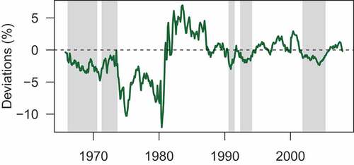
Figure 10. Markov switching: regime 1 (“Tight”).

Notes: The figure shows the periods corresponding to the first Markov switching regime conditional mean and variance for the deviations from the Taylor Rule. The fitted conditional mean and standard deviation are 0.358 and 0.722, respectively. This regime can be interpreted as “tight” regime, where the federal funds rate is higher than the recommendation from the Taylor Rule. Periods of the Greenspan and Bernanke chairmanships correspond to this regime.

The Markov-Switching model classifies Volcker and Burns in the same regime, despite the fact that Volcker was much tighter than the Taylor Rule, and Burns was much looser than the rule (Figure 11). Regime 2 can thus be interpreted as a monetary policy regime that is “inconsistent” with the Taylor Rule, and is either very tight or very loose. In Figure 11, Greenspan was “inconsistent” with the Taylor Rule for a brief period following the economic fallout from the tech stock crash and the September 2001 terrorist attacks.

Figure 11. Markov switching: regime 2 (“Inconsistent”).

Notes: The figure shows the periods corresponding to the second Markov switching regime conditional mean and variance for the deviations from the Taylor Rule. The fitted conditional mean and standard deviation are −1.546 and 4.930, respectively. This regime can be interpreted as a non-standard regime, periods where monetary policy substantially deviates from the Taylor rule. The period covers the Burns chairmanship keeping monetary policy loose at Nixon’s behest, and the Volcker chairmanship keeping monetary policy tighter than recommended due to the emphasis on fighting inflation over boosting output during his tenure. Most of Burns and all of Volcker’s tenure deviate substantially from the real-time Taylor Rule. A small portion of the Greenspan’s chairmanship post-2000 is “inconsistent” with the Taylor Rule, but he appears to have erred in being overly tight, based on the plot, rather than too loose.

The estimated conditional means and variance for the model in equation 7 are

(9) $i_{Taylor}=\left\{\begin{array}{cc}-1.856+{\in }_t,{\in }_t\sim N(0,0.764),& s_t=0\\ 0.358+{\in }_t,{\in }_t\sim N(0,0.722),& s_t=1\\ -1.546+{\in }_t,{\in }_t\sim N(0,4.930),& s_t=2\end{array}\right.$(9)

and the estimated transition matrix is

(10) $P=\left[\begin{array}{ccc}0.968& 0.007& 0.025\\ 0.014& 0.981& 0.007\\ 0.019& 0.012& 0.969\end{array}\right].$(10)

The transition matrix shows that regimes identified from fed funds deviations from the Taylor Rule are very persistent. The low probabilities of transitioning between regimes imply that changes in the monetary policy framework at any point in time are, in general, very improbable.

5.1. Text analytics

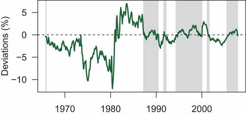
The findings of our clustering analysis (where we regard each cluster as a distinct monetary policy regime) of the FOMC meeting transcripts are presented in this section. We begin by discussing the results when only two clusters are considered, and then expand to three, four, and five clusters. Greenspan’s era is quite consistent in general.

When the FOMC transcripts are grouped into only two clusters, representing two distinct policy regimes, Figure 12 presents the results. It can be observed that there is minimal overlap between the two regimes, indicating that the chairmanships of Volcker and Greenspan are clearly distinguishable from each other. Additionally, the mean deviation from the Taylor rule for the cluster period corresponding to the Greenspan period is close to zero (−0.0211 compared to 2.93 for the other cluster), as presented in Table 4. This consistency is particularly noteworthy as it persists even when allowing for greater clustering granularity.

Figure 12. Clustering results of FOMC transcripts: 2 clusters.

Notes: The figure shows the clustering results when the FOMC transcripts are divided into 2 clusters. We interpret each cluster of similar texts as a distinct regime of monetary policy.

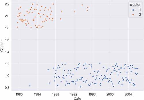
Table 4. Mean deviation from the Taylor rule: By clusters

Cluster	Mean deviation	Mean deviation	Mean deviation
	two clusters	three clusters	four clusters
Cluster 1	−0.021	−0.021	−0.021
Cluster 2	2.93	3.72	3.44
Cluster 3	-	0.557	2.54
Cluster 4	-	-	0.557

Notes: The table shows the mean deviation from the Taylor for each cluster in the case of two, three, and four clusters.

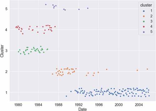
Figure 13 demonstrates the results when the FOMC transcripts are divided into three clusters. The majority of the transcripts from the Volcker era (August 1979 to August 1987) belong to the same cluster, while the Greenspan meeting transcripts are split into the remaining two clusters. The post-1990 Greenspan regime looks quite consistent as evidenced by almost all of the post-1990 documents being classified as a single regime. This consistency holds even when we allow the k-means clustering algorithm to group the transcripts into four or five clusters, as shown in Figures 14 and 15 respectively. Most of the post-1990 transcripts belong to the same cluster, and most importantly, 2003–2006 is not distinguishable as a separate policy regime during Greenspan’s tenure.

Figure 13. Clustering results of FOMC transcripts: 3 clusters.

Notes: The figure shows the clustering results when the FOMC transcripts are divided into 3 clusters. We interpret each cluster of similar texts as a distinct regime of monetary policy.

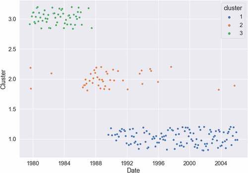
Figure 14. Clustering results of FOMC transcripts: 4 clusters.

Notes: The figure shows the clustering results when the FOMC transcripts are divided into 4 clusters. We interpret each cluster of similar texts as a distinct regime of monetary policy.

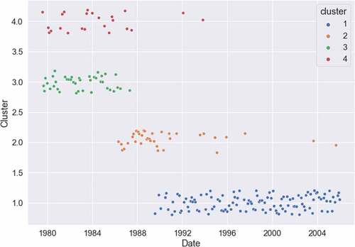
Figure 15. Clustering results of FOMC transcripts: 5 clusters.

Notes: The figure shows the clustering results when the FOMC transcripts are divided into 5 clusters. We interpret each cluster of similar texts as a distinct regime of monetary policy.

In addition, the analysis reveals that there is no clear distinction between the policy regime of 2003–2006 and the rest of Greenspan’s tenure. This implies that Greenspan’s approach to monetary policy during his final years was consistent with the policies he implemented earlier in his tenure.

In summary, the results from our clustering analysis demonstrate that Greenspan’s tenure as Federal Reserve Chair was characterized by a high degree of consistency in monetary policy. Even when using a more nuanced clustering approach, most of the post-1990 transcripts remain classified as belonging to the same policy regime. Moreover, our analysis indicates that there is no discernible difference between the policy regime of 2003–2006 and the rest of Greenspan’s tenure.

5.2. Cluster characteristics

Figures 16, 17, and 18 present the word cloud outcomes for the primary terms in clusters labeled 1, 2, and 3, respectively. The larger and bolder terms in the clouds indicate the significance of the term within the particular cluster. Although we only present the terms for the case of 3 clusters for clarity, the memberships of the clusters are generally consistent. This means that as we shift from, say, three to four clusters, just a few transcripts change their cluster memberships.

Figure 16. Wordcloud of the top texts in cluster 1 (regime from roughly from 1990 to 2007).

Notes: The figure shows the wordcloud for the top single word and two-word phrases in the first cluster. The transcripts from the later era of Greenspan’s tenure paid close attention to U.S. stock market and financial sector in general.

Figure 17. Wordcloud of the top texts in cluster 2 (regime from roughly from 1987 to 1990).

Notes: The figure shows the wordcloud for the top single word and two-word phrases in the second cluster. This cluster corresponds mostly to texts early in Greenspan’s tenure, where international trade and exchange rates relative to U.S. dollar figured prominently in the conversation.

Figure 18. Wordcloud of the top texts in cluster 3 (regime from roughly from 1979 to 1986).

Notes: The figure shows the wordcloud for the top single word and two-word phrases in the third cluster. This cluster corresponds mostly to texts in Volcker’s tenure, where the transcripts reflect the debate over the use of money supply or federal funds rate as targets, as well as the desire to reduce unemployment.

Cluster 1, which roughly corresponds to the majority of Greenspan’s tenure after 1990, features top relevant terms such as “recovery”, “stock market”, “recession”, among others. Cluster 2, covering the initial years of Greenspan’s tenure, includes terms like “exports”, “international trade”, “dollar”, “exchange”, indicating that the transcripts during this period focused on topics related to international trade and finance. In contrast, after 1990, the discussion in the transcripts seems to have heavily centered on the stock market, according to the clustering algorithm’s findings. Lastly, cluster 3, which aligns with the Volcker era, highlights top terms such as “money supply”, “federal funds”, “targets”, and “interest rate”. During the Volcker regime, which began in 1979, the discussion in the text was centered around which targets the Fed should be using, switching to targeting the money supply from 1979 to 1981 and then reverting to interest rate targets after 1981.

6. Conclusion

Alan Greenspan’s early years as the head of the Federal Reserve, spanning from 1988 to the end of 2000, were marked by remarkable consistency with the real-time Taylor Rule, with the federal funds rate oscillating around the Rule’s recommended value with low variance each month. While the second part of Greenspan’s Federal Reserve leadership was characterized by a policy that appeared to be looser than that suggested by the Taylor Rule, the conditional mean found by the Bai and Peron structural break process is still consistent across his tenure. The Markov switching regime identified the year 2003 as a “loose” period, but it was not significantly different from other “loose” periods during his tenure, or even during Martin’s chairmanship in the late 1960s.

The contention by Taylor (2007, 2009) that Greenspan inflated the housing bubble is inconsistent with a historical inspection of Federal Reserve deviations from the Taylor Rule. Greenspan had a conditional mean deviation of zero throughout his tenure, assuming a constant level of variance with Bai and Perron (2003a). A less restrictive Markov-Switching model finds that some periods of Greenspan’s tenure corresponded to “loose” monetary policy, but the conditional variance was extremely close for both the “loose” and “tight” Markov-switching regimes as Equation 9(9) $i_{Taylor}=\left\{\begin{array}{cc}-1.856+{\in }_t,{\in }_t\sim N(0,0.764),& s_t=0\\ 0.358+{\in }_t,{\in }_t\sim N(0,0.722),& s_t=1\\ -1.546+{\in }_t,{\in }_t\sim N(0,4.930),& s_t=2\end{array}\right.$(9) shows. To the extent that Greenspan deviated from the Taylor Rule, he deviated in a cyclical, symmetric manner: Negative deviations were offset by positive deviations from the Taylor Rule, which is inconsistent with Taylor’s argument that the period of 2003–2006 differed from what economic agents had come to expect of monetary policy. On the whole, we find that Greenspan’s interest rate policies were broadly consistent with the Taylor Rule. In addition, using an FOMC text-based analysis to find policy regimes, the policy discussions from 2003 to 2006 were also no different than the vast majority of policy discussions earlier in Greenspan’s tenure.

6.1. Policy Implications

The study has several policy implications worth considering. One of the main findings is that the Taylor Rule, while a useful guideline, has limitations due to data constraints, which means that strict adherence to it may not always be the best solution for addressing speculative bubbles. Additionally, it would be unwise for Congress to impose mechanical adherence to the Taylor Rule for the FOMC in setting interest rates. The study shows that the FOMC, under Greenspan’s tenure, has generally followed the Taylor Rule, taking into account the available economic data at the time of the policy decision. Therefore, any future attempts to restrict the FOMC to follow the Taylor Rule should consider the real-time data available at the time of the rate-setting decision, as this can significantly alter the implied short-term interest rates compared to the final economic data.

Acknowledgments

We gratefully acknowledge Dr. Gerald Dwyer, Dr. Robert Tamura, Dr. Michal Jerzmanowski, Dr. Aspen Gorry, Dr. Scott Baier, and all participants at Macroeconomics workshop at Clemson University. All remaining errors are ours.

Disclosure statement

This is an original manuscript, and no part of it has been published before or is under consideration at another journal. We have no relevant or material financial interests that relate to the research described in this paper.

Notes

1. Appendix A.1 discusses the procedure in detail.

Appendix A.1

From Text Documents to Numerical Feature VectorsFor clustering analysis, the text documents will first need to be converted to a vector of real numbers. We follow a three-step procedure commonly employed in natural language processing literature to transform texts to numerical vectors. First, we assign integer identification for each single word or a two word phrase, the process referred to as tokenization. Second, we counting the number of occurrences of each token for each document in the collection of FOMC documents. Finally, we normalize each document to have a feature matrix of the same size and also weight tokens that occur in the majority of documents with diminishing importance. We use tf-idf method by Salton and McGill (1983) to obtain weights for each token.

In order to calculate tf-idf value of a token in each document, we multiply the frequency of that token by its idf component. The idf frequency is given by

(11) $idf(t)=log\frac{(1+n_d)}{1+df(d,t)}+1,$(11)

where $n_d$ is the total number of documents, and df(d,t) is the number of documents that contain term $t$. The tf-idf vectors are then normalized by the Euclidean norm and is given by

(12) $v_{norm}=\frac{v}{\sqrt{{(v_1)}^2+{(v_2)}^2+\dots +{(v_n)}^2}}.$(12)

Upon completion of this 3-step procedure, we obtain a features matrix $X$, a row of which consists of tf-idf values of all tokens for each document in our collection of documents. Each row is also normalized to have a unit norm to account for the fact that documents are of variable length. Otherwise, a longer document will have higher term frequencies and thus higher tf-idf values than a shorter document.

Appendix

K-means Clustering Algorithm

This section closely follows James et al. 2013. Let $X=\{x_i\}$, $x_i\in {\mathbb{R}}^{\mathbb{D}}$, be the set of FOMC transcripts to be clustered into a set of K clusters, $C=\{c_k:k=1,..,K\}$ where $D$ is the number of features per transcript. We assume a-priori that there exists $K$ clusters with cluster centers ${\mu }_1,{\mu }_2,\dots ,{\mu }_k\in {\mathbb{R}}^{\mathbb{D}}$. K-means clustering solves

(13) $\underset{C}{\mathrm{a}\mathrm{r}\mathrm{g}\mathrm{m}\mathrm{a}\mathrm{x}}\sum _{i=1}^K\sum _{x\in c_i}\parallel \mathbf{x}-{\mu }_{\mathbf{i}}{\parallel }^2.$(13)

The optimization algorithm takes place in the following steps.

1. Choose the number of clusters, $k$, that we would like the texts to be split into based on domain knowledge.

2. Arbitrarily initialize cluster centers ${\mu }_1,{\mu }_2,\dots ,{\mu }_k$.

3. Given the fixed cluster centers, choose optimal cluster assignment for each data point (FOMC transcript) $x_i$ based on the closest cluster center.

4. Update ${\mu }_1,{\mu }_2,\dots ,{\mu }_k$ on the basis of cluster assignments of $x_i$.

5. Repeat steps 3 and 4 until convergence takes place, i.e. the centroids of the cluster do not move.

We repeat the steps outlined above for different values of $K$, namely 2, 3, 4, and 5.

Appendix

Figure A1. Within Groups Sums of Squares.

References

- Abel, A. B., Bernanke, B. S., & Dean, C. (2005). Macroeconomics. Pearson.
- Alba, J. D., & Wang, P. (2017). Taylor rule and discretionary regimes in the United States: Evidence from a k-state Markov regime-switching model. Macroeconomic Dynamics, 21(3), 817–24. https://doi.org/10.1017/S1365100515000693
- Alex, N.R., Papell, D. H., & Prodan, R. (2019). The Taylor principles. Journal of Macroeconomics, 62, 103159.
- Athanasios, O., & Williams, J. C. (2003). Monetary policy rules and the Great Inflation. The American Economic Review, 93(3), 545–569.
- Bai, J., & Perron, P. (1998). Estimating and testing linear models with multiple structural changes. Econometrica, 66(1), 47–78. https://doi.org/10.2307/2998540
- Bai, J., & Perron, P. (2003a). Computation and analysis of multiple structural change models. Journal of Applied Econometrics, 18(1), 1–22. https://doi.org/10.1002/jae.659
- Bai, J., & Perron, P. (2003b). Critical values for multiple structural change tests. The Econometrics Journal, 6(1), 72–78. https://doi.org/10.1111/1368-423X.00102
- Board of the Governors of the Federal Reserve System. (2021) (Retrieved February 12, 2021) FOMC Transcripts and Other Historical Materials. https://www.federalreserve.gov/monetarypolicy/fomchistorical2011.htm
- Boivin, J. (2006). Has US monetary policy changed? Evidence from drifting coefficients and real-time data. Journal of Money, Credit, and Banking, 38(7), 1149–1173. https://doi.org/10.1353/mcb.2006.0065
- Clarida, R., Gali, J., & Gertler, M. (1999). The science of monetary policy: A new Keynesian perspective. Journal of Economic Literature, 37(4), 1661–1707. https://doi.org/10.1257/jel.37.4.1661
- Cooley, T. F., & Prescott, E. C. (1976). Estimation in the presence of stochastic parameter variation. Econometrica, 44(1), 167–184. https://doi.org/10.2307/1911389
- Diebold, F. X., Lee, J.H., & Weinbach, G. C. (1994). Regime switching with time-varying transition probabilities. Business Cycles: Durations, Dynamics, and Forecasting, 1, 144–165.
- Engel, C. (1994). Can the Markov switching model forecast exchange rates? Journal of International Economics, 36(1–2), 151–165. https://doi.org/10.1016/0022-1996(94)90062-0
- Engel, C., & Hamilton, J. D. (1990). Long swings in the dollar: Are they in the data and do markets know it? The American Economic Review, 80, 689–713.
- Fair, R. C. (2001). Actual federal reserve policy behavior and interest rate rules. Federal Reserve Bank of New York Economic Policy Review, 7(1), 61–72.
- Filardo, A. J. (1994). Business-cycle phases and their transitional dynamics. Journal of Business & Economic Statistics, 12(3), 299–308. https://doi.org/10.1080/07350015.1994.10524545
- Garcia, R., & Perron, P. (1996). An analysis of the real interest rate under regime shifts. The Review of Economics and Statistics, 78(1), 111–125. https://doi.org/10.2307/2109851
- Ghysels, E. (1994). On the periodic structure of the business cycle. Journal of Business & Economic Statistics, 12(3), 289–298. https://doi.org/10.1080/07350015.1994.10524544
- Goodwin, T. H. (1993). Business-cycle analysis with a Markov-switching model. Journal of Business & Economic Statistics, 11(3), 331–339. https://doi.org/10.1080/07350015.1993.10509961
- Hamilton, J. D. (1988). Rational-expectations econometric analysis of changes in regime: An investigation of the term structure of interest rates. Journal of Economic Dynamics and Control, 12(2–3), 385–423. https://doi.org/10.1016/0165-1889(88)90047-4
- Hamilton, J. D. (1989). A new approach to the economic analysis of nonstationary time series and the business cycle. Econometrica: Journal of the Econometric Society, 57(2), 357–384. https://doi.org/10.2307/1912559
- Handlan, A. (2021). Text shocks and monetary surprises (Doctoral dissertation, University of Minnesota).
- Hansen, B. E. (2001). The New Economnetrics of Structural Change: Dating Breaks in U.S. Labor Productivity. Journal of Economic Perspectives, 15(4), 117–128.
- Hansen, S., & McMahon, M. (2016). Shocking language: Understanding the macroeconomic effects of central bank communication. Journal of International Economics, 99, S114–133. https://doi.org/10.1016/j.jinteco.2015.12.008
- Judd, J. P., & Rudebusch, G. D. (1998). Taylor’s rule and the fed: 1970-1997. Economic Review–Federal Reserve Bank of San Francisco, 3, 3–16.
- Kim, C.J., & Nelson, C. R. (1998). Business cycle turning points, a new coincident index, and tests of duration dependence based on a dynamic factor model with regime switching. The Review of Economics and Statistics, 80(2), 188–201. https://doi.org/10.1162/003465398557447
- Kim, M.J., & Yoo, J.S. (1995). New index of coincident indicators: A multivariate Markov switching factor model approach. Journal of Monetary Economics, 36(3), 607–630. https://doi.org/10.1016/0304-3932(95)01229-X
- Lam, P.S. (1990). The Hamilton model with a general autoregressive component: Estimation and comparison with other models of economic time series: Estimation and comparison with other models of economic time series. Journal of Monetary Economics, 26(3), 409–432. https://doi.org/10.1016/0304-3932(90)90005-O
- Mehra, Y. P., & Sawhney, B. (2010). Inflation measure, Taylor rules, and the Greenspan-Bernanke years. FRB Richmond Economic Quarterly, 96(2), 123–151.
- Murray, C. J., Nikolsko-Rzhevskyy, A., & Papell, D. H. (2015). Markov switching and the Taylor principle. Macroeconomic Dynamics, 19(4), 913–930.
- Orphanides, A. (2001). Monetary policy rules based on real-time data. The American Economic Review, 91(4), 964–985.
- Orphanides, A. (2002). Monetary-policy rules and the great inflation. The American Economic Review, 92(2), 115–120.
- Orphanides, A., & Wieland, V. (2008). Economic projections and rules-of-thumb for monetary policy. Federal Reserve Bank of St Louis Review, 90(July/August), 307–324.
- Primiceri, G. E. (2005). Time varying structural vector autoregressions and monetary policy. The Review of Economic Studies, 72(3), 821–852.
- Quandt, R. E. (1972). A new approach to estimating switching regressions. Journal of the American Statistical Association, 67(338), 306–310.
- Salton, G., & McGill, M. J. (1983). Introduction to modern information retrieval. McGraw-Hill.
- Schaller, H., & Van Norden, S. (1997). Regime switching in stock market returns. Applied Financial Economics, 7(2), 177–191.
- Shapiro, A. H., & Wilson, D. J. (2022). Taking the fed at its word: A new approach to estimating central bank objectives using text analysis. The Review of Economic Studies, 89(5), 2768–2805.
- Sims, C. A. (1980). Macroeconomics and reality. Econometrica, 48(1), 1–48.
- Sims, C. A. (1992). Interpreting the macroeconomic time series facts: The effects of monetary policy. European Economic Review, 36(5), 975–1000.
- Sims, C. A., & Zha, T. (2006). Were there regime switches in US monetary policy? The American Economic Review, 96(1), 54–81.
- Sola, M., & Driffill, J. (1994). Testing the term structure of interest rates using a stationary vector autoregression with regime switching. Journal of Economic Dynamics and Control, 18(3–4), 601–628.
- Svensson, L. E. O. (2017). Monetary policy with judgment: Forecast targeting. International Journal of Central Banking, 1(1), 1–54.
- Taylor, J. B. (1993) Discretion versus policy rules in practice. In Carnegie-Rochester Conference Series on Public Policy, 39, 195–214.
- Taylor, J. B. (1999). A historical analysis of monetary policy rules. In John B. Taylor (Ed.), Monetary Policy Rules (pp. 319–348). University of Chicago Press.
- Taylor, J. B. (2007). Housing and monetary policy. No. w13682National Bureau of Economic Research.
- Taylor, J. B. 2009. The financial crisis and the policy responses: An empirical analysis of what went wrong. Working Paper 14631. National Bureau of Economic Research (January).
- Timothy, C., & Sargent, T. J. (2005). Drifts and volatilities: Monetary policies and outcomes in the post WWII US. Review of Economic Dynamics, 8(2), 262–302. https://doi.org/10.1016/j.red.2004.10.009
- Westelius, N. J. (2007). The time-varying nature of the link between inflation and inflation uncertainty: Evidence from the US, UK and Germany. Journal of International Money & Finance, 26(7), 1146–1165.
- Yoosoon, C., Choi, Y., & Park, J. Y. (2017). A new approach to model regime switching. Journal of Econometrics, 196(1), 127–143. https://doi.org/10.1016/j.jeconom.2016.09.005